A Nonlinear Subspace Predictive Control Approach Based on Locally Weighted Projection Regression

Abstract

Subspace predictive control (SPC) is a widely recognized data-driven methodology known for its reliability and convenience. However, effectively applying SPC to complex industrial process systems remains a challenging endeavor. To address this, this paper introduces a nonlinear subspace predictive control approach based on locally weighted projection regression (NSPC-LWPR). By projecting the input space into localized regions, constructing precise local models, and aggregating them through weighted summation, this approach handles the nonlinearity effectively. Additionally, it dynamically adjusts the control strategy based on online process data and model parameters, while eliminating the need for offline process data storage, greatly enhancing the adaptability and efficiency of the approach. The parameter determination criteria and theoretical analysis encompassing feasibility and stability assessments provide a robust foundation for the proposed approach. To illustrate its efficacy and feasibility, the proposed approach is applied to a continuous stirred tank heater (CSTH) benchmark system. Comparative results highlight its superiority over SPC and adaptive subspace predictive control (ASPC) methods, evident in enhanced tracking precision and predictive accuracy. Overall, the proposed NSPC-LWPR approach presents a promising solution for nonlinear control challenges in industrial process systems.

1. Introduction

Industrial processes constitute the backbone of modern economies, contributing to diverse sectors such as chemical engineering, transportation, and energy production [1,2,3]. The efficient operation and regulation of these processes are essential for achieving optimal resource utilization, product quality, and safety [4]. In pursuit of these objectives, the field of industrial process control has emerged as a crucial discipline, aiming to harness advancements in science and technology to enhance process performance, stability, and reliability [5].

The significance of industrial process control extends beyond mere operational efficiency. It plays a pivotal role in ensuring consistent product quality, minimizing waste, and mitigating environmental impact [6,7,8]. Furthermore, effective control strategies empower industries to adapt swiftly to changing market demands and regulatory requirements, fostering competitiveness and sustainability [9]. However, the realm of industrial process control is not without its challenges. Conventional model-based control approaches encounter limitations when applied to complex industrial systems [10,11,12]. A prominent constraint is the difficulty in obtaining accurate and comprehensive model information. Constructing a detailed mathematical representation for complex processes is often formidable, especially given nonlinear dynamics, intricate interactions, and inherent uncertainties [13]. These challenges hinder the efficacy of conventional model-based control, leading to suboptimal performance, compromised stability, and difficulties in real-time adaptation [14].

To tackle these formidable challenges, data-driven control approaches have emerged as a promising and dynamic solution in the realm of industrial process control [15]. These methodologies, including machine learning [16], deep learning [17], and reinforcement learning [18], leverage the wealth of information derived from sensors, actuators, and historical data to formulate effective and adaptive control strategies.

Within the spectrum of data-driven control strategies, the subspace predictive control (SPC) approach stands out as a particularly compelling choice. SPC ingeniously combines subspace identification techniques with predictive control methodologies, rendering it an attractive option for its simplicity and ease of implementation [19]. The adoption of SPC has spurred extensive research into its practical applications within the realm of industrial process control. For instance, Li et al. [20] have devised a SPC method to regulate the power allocation of server racks and control the supply temperature of cold air. Furthermore, Navalkar et al. [21] have introduced a repetitive SPC approach that demonstrates precise individual blade pitch control on a wind turbine prototype. These applications underscore the potential of SPC in optimizing complex industrial systems. Nevertheless, it remains clear that many intricate industrial systems inherently exhibit nonlinear behaviors, intricate interactions, and uncertain dynamics. While the strength of SPC lies in its foundation on linear models and its reliance on offline data, it encounters formidable challenges when confronted with the inherent complexities of nonlinear processes. This limitation has the potential to curtail its effectiveness in capturing the multifaceted nature of these systems and responding adeptly to dynamic variations [22].

To address the prevalent issue of the inadequacy of the SPC method in dealing with the intricate nonlinear dynamics inherent in industrial processes, there is a compelling imperative to develop and advance the field of adaptive subspace predictive control (ASPC). The primary objective motivating ASPC is to facilitate real-time adjustments of controller parameters in response to dynamic data fluctuations, offering a dynamic and adaptive approach to control. A cornerstone of ASPC involves the utilization of a sliding data window mechanism, which serves as a vital tool for describing the current operational conditions and effectively mitigating the nonlinear complexities often encountered in intricate systems. This approach has been notably applied and refined by pioneering researchers such as Wahab et al. [23], Vajpayee et al. [24], and Hallouzi et al. [25]. Their work has showcased the effectiveness of the sliding data window in applications ranging from wastewater treatment systems to nuclear reactors and even complex models like the Boeing 747 aircraft. While substantial progress has been achieved in the application of ASPC, a noteworthy limitation lies in the fact that these methodologies have predominantly been tailored to linear controllers. This limitation restricts their capability to comprehensively address the intricate nonlinear characteristics commonly found in diverse industrial scenarios.

To achieve a more robust and appropriate solution, some researchers have explored alternative avenues by directly crafting controllers explicitly designed for specific nonlinear systems. For example, a specialized nonlinear subspace predictive controller tailored to bilinear systems is introduced in [26]. Zhou et al. [27] and Luo et al. [28] have extended nonlinear SPC methods to encompass Hammerstein systems and Hammerstein–Wiener systems, expanding the scope of applicability. However, it is essential to recognize that while these endeavors have shown promise, designing controllers for specific nonlinear systems often lacks the necessary universality required for broad industrial implementation. In light of these considerations, the field of nonlinear SPC is confronted with the challenge of achieving a more versatile solution.

In this paper, a nonlinear subspace predictive control approach based on locally weighted projection regression (NSPC-LWPR) is presented to address the aforementioned issues. The locally weighted projection regression (LWPR) algorithm, which is an incremental nonparametric statistical learning technique [29] and is related to the field of linear parameter varying modeling [30,31,32], is integrated into the SPC method. By fitting the local nonlinear relationships between input and output data to construct a predictive model, higher prediction accuracy can be achieved when the expected output of the nonlinear process changes, while maintaining smooth tracking. The main contributions of this approach are listed as follows:

(1)

Seamless integration of LWPR and SPC: The LWPR algorithm and the SPC method are seamlessly integrated for industrial process control. By projecting the input space into localized regions, constructing precise local models, and aggregating them through weighted summation, the proposed approach effectively addresses the complex nonlinear relationships in industrial processes.

(2)

Enhanced adaptability and efficiency: The proposed approach constructs the controller from the trained regression model. This implies that it can adapt the control strategy using online process data and local model parameters. In addition, it removes the necessity for storing offline process data. These advancements highlight improvements in both adaptability and efficiency.

(3)

Improved predictive and tracking performance: The proposed approach shows improvements in both predictive and tracking performance. It creates an accurate predictive model by capturing the dynamic characteristics of the system from input/output (I/O) data. This boosts the accuracy of the predictive controller, especially during transitions from nonlinear to steady-state processes. The increased prediction accuracy also greatly enhances the tracking performance of the predictive controller. In situations where the expected output of the nonlinear process changes, the controlled system adjusts smoothly to match the projected output path, ensuring consistent and smooth tracking.

This paper is structured as follows. Section 2 offers an extensive elucidation of the preliminaries associated with the subspace predictor and the LWPR learning scheme. Section 3 focuses on the design of the controller, including parameter determination criteria and theoretical analysis. The application of the proposed NSPC-LWPR approach in a CSTH benchmark study is showcased in Section 4. Finally, Section 5 concludes the paper by summarizing its main content and suggesting potential directions for future research.

2. Preliminaries

2.1. Subspace Predictor

Assuming discrete time intervals indexed by k where measurements of the I/O data for the system are denoted by $u_k\in {\mathbb{R}}^m$ and $y_k\in {\mathbb{R}}^l$, the stacked vector $u_{s,k}$ of length s is introduced as

$$u_{s,k}={\left[\begin{array}{ccc}{u}_k^T& \cdots & u_{k+s-1}^T\end{array}\right]}^T.$$

(1)

The block Hankel matrices $U_p$ and $U_f$ are constructed as

$$\begin{array}{cc}\hfill U_p& =\left[\begin{array}{ccc}{u}_{s_p,k-s_p+1}& \cdots & u_{s_p,k-s_p+\overline{N}}\end{array}\right],\hfill \\ \hfill U_f& =\left[\begin{array}{ccc}{u}_{s_f,k+1}& \cdots & u_{s_f,k+\overline{N}}\end{array}\right],\hfill \end{array}$$

(2)

where the indexes p and f correspond to the past and future block Hankel matrices, respectively. $s_p$ and $s_f$ both denote the number of row blocks. $\overline{N}$ represents the sample length. Similarly, the output data block Hankel matrices $Y_p$ and $Y_f$ are defined based on the output data.

The subspace predictor model represents the optimal prediction of $Y_f$ as a combination of past I/O data and future input data [33]. The subspace predictor can be formulated as

$${\widehat{Y}}_f=L_w{W}_p+L_u{U}_f,$$

(3)

where $L_w$ and $L_u$ are the subspace predictor coefficient matrices, and $W_p={\left[{\left(Y_p\right)}^T{\left(U_p\right)}^T\right]}^T$.

2.2. LWPR Learning Scheme

The LWPR algorithm employs the standard regression model $y={\beta }^{\mathtt{T}}x+\epsilon$ to approximate the nonlinear function $y=f\left(x\right)+\epsilon$, where x is the input vector, y is the scalar output, and $\epsilon$ is a zero-mean random noise term.

To capture the locality aspect, the position of each data point x is leveraged through a Gaussian kernel to compute the weight w:

$$w=exp\left(-0.5{(x-x_c)}^{\mathtt{T}}D(x-x_c)\right),0<w\le 1,$$

(4)

where $x_c$ denotes the center of a local subset of data, and D is a positive semi-definite distance metric that determines both the size and shape of the neighborhood contributing to the establishment of the corresponding local model. A smaller D results in a smoother kernel, while a larger D captures finer details. As discussed in [34], besides the Gaussian kernel, alternative kernel functions can also be employed. However, the choice of kernel function only affects the computation of weights and consequently influences the number and shape of local models, but it does not significantly impact the prediction results.

Based on the obtained weights, the following weighted means can be calculated:

$$\overline{x}=\sum _{n=1}^N{w}_n{x}_n/\sum _{n=1}^N{w}_n,\overline{y}=\sum _{n=1}^N{w}_n{y}_n/\sum _{n=1}^N{w}_n.$$

(5)

By subtracting $\overline{x}$ and $\overline{y}$ from the original measurements, the input and output of the LWPR algorithm can be guaranteed with zero means.

Following the initialization of LWPR without a locally linear model (receptive field, RF), the algorithm proceeds with the training process. For each training sample, the weight is computed using (4). Subsequently, the regressions, projections, and distance metrics of each RF are updated iteratively until no new RF creation is required. The crucial aspects of the LWPR learning scheme for one RF centered at $x_c$, which hold relevance for our extension of locally weighted learning to SPC, are concisely summarized in

Table 1. Locally Weighted Projection Regression (LWPR) learning scheme for one RF centered at $x_c$ [29].

1. Initialization: (number of training samples seen $n=0$)

$x_0^0=0,{\beta }_0^0=0,W^0=0,u_r^0=0,p_r^0=0;r=1:R$

2. Incorporating new data: Given training point(x,y)

2a. Compute activation and update the means

1.$w=exp\left(-0.5{\left(x-x_c\right)}^{T}D\left(x-x_c\right)\right);W^{n+1}=\lambda W^n+w$

2.$x_0^{n+1}=\left(\lambda W^n{x}_0^n+wx\right)/W^{n+1}$;

${\beta }_0^{n+1}=\left(\lambda W^n{\beta }_0^n+wy\right)/W^{n+1}$

2b. Compute the current prediction error

$x_{res,1}=x-x_0^{n+1},\widehat{y}={\beta }_0^{n+1}$

Repeat for $r=1:R$(projections)

$\begin{array}{c}1.z_r=x_{\mathrm{res},r}^T{u}_r^n/\sqrt{{u_r^n}^T{u}_r^n}\hfill \\ 2.\widehat{y}=\widehat{y}+{\beta }_r^n{z}_r\hfill \\ 3.x_{\mathrm{res},r+1}=x_{\mathrm{res},r}-z_r{p}_r^n\hfill \\ 4.{\mathrm{MSE}}_r^{n+1}=\lambda {\mathrm{MSE}}_r^n+w{\left(y-\widehat{y}\right)}^2\hfill \end{array}$

2c. Update the local model

${\mathrm{res}}_1=y-{\beta }_0^{n+1}$

Repeat for $r=1:R$(projections)

2c.1 Update the local regression and compute residuals

$\begin{array}{c}1.a_{zz,r}^{n+1}=\lambda a_{zz,r}^n+w{z}_r^2;a_{zres,r}^{n+1}=\lambda a_{zres,r}^n+w{z}_{r}re{s}_r\hfill \\ 2.{\beta }_r^{n+1}=a_{\mathrm{zres},r}^{n+1}/a_{\mathrm{zz},r}^{n+1}\hfill \\ 3.{\mathrm{res}}_{r+1}={\mathrm{res}}_r-z_r{\beta }_r^{n+1}\hfill \\ 4.a_{\mathrm{xz},r}^{n+1}=\lambda a_{\mathrm{xz},r}^n+w{x}_{\mathrm{res},r}{z}_r\hfill \end{array}$

2c.2 Update the projection directions

$1.u_r^{n+1}=\lambda u_r^n+w{x}_{\mathrm{res},r}{\mathrm{res}}_r$

$2.p_r^{n+1}=a_{\mathrm{xz},r}^{n+1}/a_{\mathrm{zz},r}^{n+1}$

. Corresponding symbols and their notations are provided in

Table 2. Indexes and symbols used for LWPR [29].

Notation	Description
N	Number of training data points
M	Number of local models
R	Number of local projections
$z_r(r=1:A)$	rth element of the lower-dimensional projection of input data x
${\mathrm{u}}_r(r=1:A)$	rth projection direction
${\mathrm{p}}_r(r=1:A)$	Regressed input space to be subtracted to maintain orthogonality of projection directions
W	Diagonal weight matrix representing the activation due to all samples
${\beta }_r(r=1:A)$	rth component of slope of the local linear model $\beta ={\left[\begin{array}{ccc}{\beta }_1& \cdots & {\beta }_R\end{array}\right]}^T$
$\lambda$	Forgetting factor used to exclude data and accelerate the learning process
${\mathrm{MSE}}_r^n$	Mean square error of the nth sample in the rth projection
$a_{\mathrm{zz},r}^n,a_{\mathrm{zres},r}^n,a_{\mathrm{xz},r}^n$	Sufficient statistics for incremental computation of rth dimension of variable var after seeing n data points

.

3. Locally Weighted Projection Regression-Based Subspace Predictive Control

3.1. Controller Design

Considering that only the leftmost column of ${\widehat{Y}}_f$ is considered to predict the output, (3) can be rewritten as

$${\widehat{y}}_{N_{p}l}={\tilde{L}}_w{w}_p+{\tilde{L}}_u{u}_{N_{c}m},$$

(6)

where ${\widehat{y}}_{N_{p}l}$ is the first $N_{p}l$ row of the leftmost column in ${\widehat{Y}}_f$, $w_p$ is the leftmost column of $W_p$, and $u_{N_{c}m}$ is the first $N_{c}m$ row of the leftmost column in $u_f$. ${\tilde{L}}_w$ and ${\tilde{L}}_u$ are truncated from $L_w$ and $L_u$.

Given the congruity in structure between the subspace predictor outlined in (3) and the regression model employed for approximating nonlinear functions within the framework of the LWPR algorithm, it follows that the LWPR algorithm becomes instrumental in the computation of the coefficients ${\tilde{L}}_w$ and ${\tilde{L}}_u$ for the subspace predictor. Then, for the query point $u_{N_{c}m}$, the calculation of the i-th element of its output vector ${\widehat{y}}_{N_{p}l}^i$ in the local prediction output ${\widehat{y}}_{N_{p}l}^{i,j}$ of the j-th locally linear model can be simplified as follows:

$${\widehat{y}}_{N_{p}l}^{i,j}={\beta }_0^i+\sum _{r=1}^R{\beta }_r^{i,j}{s}_r^{i,j},$$

(7)

where $1\le i\le N_{p}l$, $1\le j\le M$, ${\beta }_0^i$ is the average of the i-th training output samples calculated in (5). ${\beta }_r^{i,j}$ signifies the parameter linked to the respective RF, while $s_r^{i,j}$ is defined as

$$\begin{array}{c}{s}_1^{i,j}={\left(u_1^{i,j}\right)}^T\vartheta ,\hfill \\ s_2^{i,j}={\left(u_2^{i,j}\right)}^T\left(I-p_1^{i,j}{\left(u_1^{i,j}\right)}^T\right)\vartheta ,\hfill \\ ⋮\hfill \\ s_R^{i,j}={\left(u_R^{i,j}\right)}^T\left({\displaystyle \prod _{r=R-1}^1}\left(I-p_r^{i,j}{\left(u_r^{i,j}\right)}^T\right)\right)\vartheta ,\hfill \end{array}$$

(8)

where $\vartheta =u_{N_{c}m}-{\tilde{u}}_{N_{c}m}$, and ${\tilde{u}}_{N_{c}m}$ is the average of the training input samples.

Then, ${\widehat{y}}_{N_{p}l}^{i,j}$ can be rewritten as

$${\widehat{y}}_{N_{p}l}^{i,j}={\zeta }^{i,j}+L^{i,j}{u}_{N_{c}m},$$

(9)

where

$${\zeta }^{i,j}={\beta }_0^i-\sum _{r=1}^R{\psi }_{\tau }{\tilde{u}}_{N_{c}m},L^{i,j}=\sum _{r=1}^R{\psi }_r,$$

(10)

$${\psi }_r=\left\{\begin{array}{c}{\beta }_1^{i,j}{\left(u_1^{i,j}\right)}^T,r=1\hfill \\ {\beta }_r^{i,j}{\left(u_r^{i,j}\right)}^T\left({\displaystyle \prod _{d=r-1}^1}\left(I-p_d^{i,j}{\left(u_d^{i,j}\right)}^T\right)\right).r\ne 1\hfill \end{array}\right.$$

(11)

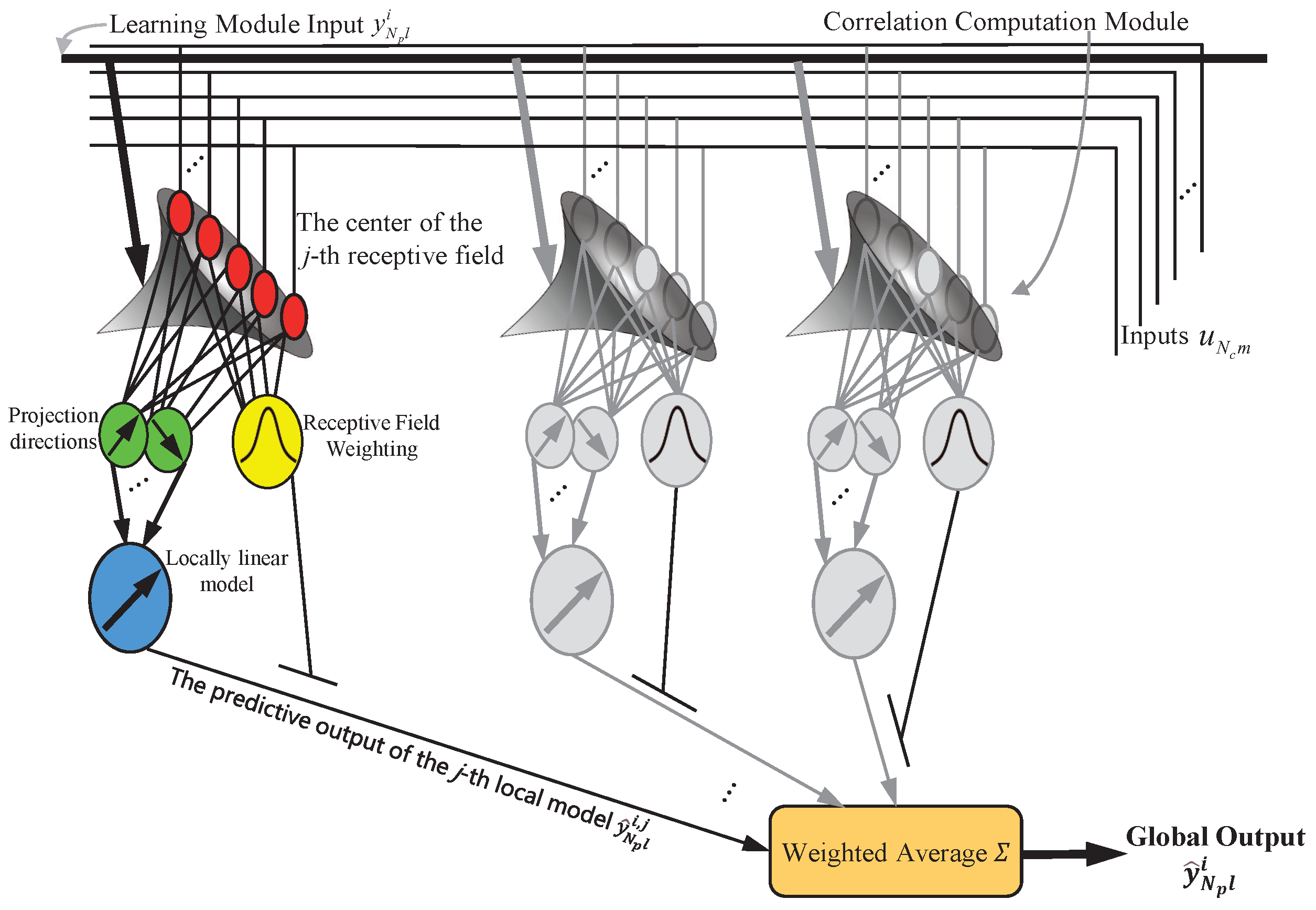
Based on the obtained weights, the total output ${\widehat{y}}_{N_{p}l}^i$ of the LWPR model is the normalized weighted mean of all the predicted outputs ${\widehat{y}}_{N_{p}l}^{i,j}$ of the M local models, that is,

$${\widehat{y}}_{N_{p}l}^i=\sum _{j=1}^M{\omega }_j{\widehat{y}}_{N_{p}l}^{i,j}/\sum _{j=1}^M{\omega }_j.$$

(12)

To better understand the solving process of global output ${\widehat{y}}_{N_{p}l}^i$, the information processing unit of the LWPR learning scheme is shown in Figure 1.

Furthermore, we have

$${\widehat{y}}_{N_{p}l}^i=L_{cst}^i+L_{cft}^i{u}_{N_{c}m},$$

(13)

where

$$L_{cst}^i=\sum _{j=1}^M{\omega }_j{\zeta }^{i,j}/\sum _{j=1}^M{\omega }_j,L_{cft}^i=\sum _{j=1}^M{\omega }_j{L}^{i,j}/\sum _{j=1}^M{\omega }_j.$$

(14)

Then, ${\widehat{y}}_{N_{p}l}$ can be expressed as

$${\widehat{y}}_{N_{p}l}=L_{cst}+L_{cft}{u}_{N_{c}m}$$

(15)

where

$$\begin{array}{c}{L}_{cst}={\left[\begin{array}{ccccc}{\left(L_{cst}^1\right)}^T& \cdots & {\left(L_{cst}^i\right)}^T& \cdots & {\left(L_{cst}^{N_{p}l}\right)}^T\end{array}\right]}^T,\hfill \\ L_{cft}={\left[\begin{array}{ccccc}{\left(L_{cft}^1\right)}^T& \cdots & {\left(L_{cft}^i\right)}^T& \cdots & {\left(L_{cft}^{N_{p}l}\right)}^T\end{array}\right]}^T.\hfill \end{array}$$

(16)

To enhance the precision of the system’s behavior modeling and maintain the consistent accuracy of predictions, it is advisable to express the projected output in (13) through an incremental formulation concerning $\Delta u_{N_{c}m}$:

$${\widehat{y}}_{N_{p}l}=A_{N_{p}l}^1{y}_k+A_{N_{p}l}^2{L}_{cft}\Delta u_{N_{c}m},$$

(17)

where

$$\begin{array}{cc}\hfill A_{N_{p}l}^1=& \left[\begin{array}{c}{I}_l\\ I_l\\ ⋮\\ I_l\end{array}\right],A_{N_{p}l}^2=\left[\begin{array}{cccc}{I}_l& 0& \cdots & 0\\ I_l& I_l& \cdots & 0\\ ⋮& ⋮& \ddots & ⋮\\ I_l& I_l& \cdots & I_l\end{array}\right],\hfill \\ \hfill \Delta u_{N_{c}m}=& {\left[{\left(\Delta u_{k+1}\right)}^T{\left(\Delta u_{k+2}\right)}^T\cdots {\left(\Delta u_{k+N_{c}m}\right)}^T\right]}^T,\hfill \end{array}$$

(18)

while $I_l$ is the identity matrix in the dimension of l, and $\Delta u_{k+1}$ in $\Delta u_{N_{c}m}$ is defined as

$$\Delta u_{k+1}=u_{k+1}-u_k,$$

(19)

and other components, such as $\Delta u_{k+2}$ and $\Delta u_{k+N_{c}m}$, are defined similarly as $\Delta u_{k+1}$.

The approach is designed to generate a control signal $u_k$ by minimizing a quadratic cost function J. This cost function takes into account the incremental input $\Delta u_k$, the provided reference signal $r_k$, and the projected output ${\widehat{y}}_k$, and is mathematically expressed as follows:

$$\begin{array}{cc}\hfill J& =\sum _{n_i=1}^{N_p}{\left(\tilde{Q}\right)}^T{W}_Q\left(\tilde{Q}\right)+\sum _{n_j=1}^{N_c}{\left(\tilde{R}\right)}^T{W}_R\left(\tilde{R}\right),\hfill \end{array}$$

(20)

where

$$\tilde{Q}=r_{k+n_i}-{\widehat{y}}_{k+n_i},\tilde{R}=\Delta u_{k+n_j},$$

(21)

while $N_p$ and $N_c$ are the prediction and control horizons. $W_Q$ and $W_R$ are the weighting matrices of the cost function J.

Based on (20) and (17), J can be rewritten as

$$J={\left(\overline{Q}\right)}^T{W}_Q\left(\overline{Q}\right)+{\left(\overline{R}\right)}^T{W}_R\left(\overline{R}\right),$$

(22)

where $\overline{Q}$ and $\overline{R}$ are represented as

$$\overline{Q}=A_{N_{p}l}^1\left(r_k-y_k\right)+A_{N_{p}l}^2{\tilde{L}}_u\Delta u_{N_{c}m},\overline{R}=\Delta u_{N_{c}m}.$$

(23)

Based on (22), it becomes evident that the cost function is exclusively contingent upon $\Delta u_{N_{c}m}$, a quantity attainable through the computation of the derivative of the cost function with respect to $\Delta u_{N_{c}m}$ under unconstrained circumstances (UCs). Furthermore, the differential quandary can be redefined as a quadratic problem under constrained circumstances (CCs). Consequently, the representation of $\Delta u_{N_{c}m}$ takes the form:

$$\Delta u_{N_{c}m}=\left\{\begin{array}{c}\frac{\partial J}{\partial \Delta u_{N_{c}m}}=0,\hfill \\ \underset{\Delta u_{N_{c}m}}{min}Js.t.A_{QP}\le B_{Qp},\hfill \end{array}\begin{array}{c}UC\\ CC\end{array}\right.$$

(24)

where $A_{QP}$ and $B_{QP}$ are constructed from preset constraints.

Upon acquiring $\Delta u_{N_{c}m}$, the initial m components are chosen for utilization. Drawing from (19) and armed with the understanding of $u_k$ as well as $\Delta u_{k+1}$, one can ascertain the forthcoming controller output to be incorporated into the regulated system, thereby determining $u_{k+1}$.

Subsequently, the control diagram outlining the proposed NSPC-LWPR approach is depicted in Figure 2, while Algorithm 1 succinctly encapsulates the essential steps.

Notably, the training of this locally weighted regression model is closely related to the number of inputs and outputs of the MIMO system. Specifically, the number of inputs and outputs directly impacts the training cost and computational efficiency of the algorithm. In essence, a larger number of inputs and outputs in the MIMO system increases the model’s training cost, reduces the computational efficiency, and prolongs the runtime. Conversely, a small number will have the opposite effect.

Algorithm 1 The proposed NSPC-LWPR approach.

Step 1. Initialization a. Fully excite the initialization signal of the system input; b. Initialize the LWPR model with no RF; Step 2. LWPR Regression Model Training a. Normalize the process data; b. Train the LWPR regression model utilizing the learning scheme specified in II-B; c. Continue the training until the predicted output of the controlled object consistently converges to its actual value; Step 3. Subspace Predictor Construction a. Calculate the subspace predictor’s coefficients according to (16); b. Convert the predictor to the incremental form of (17); Step 4. Control Input Signal Calculation a. Select methods to find $\Delta u_{N_{c}m}$ based on (24); b. Calculate the control input according to (19); c. Denormalize the solved control signal and input it into the controlled system; Step 5. Judgment a. If the controlled system is still running, return to Step 2 and calculate the next signal; b. If the controlled system stops running, the proposed approach is terminated and the calculation of the next control signal is stopped.

Furthermore, to emphasize the superiority of the proposed NSPC-LWPR approach, a theoretical comparison is performed between it and the MPC, SPC, and ASPC methods as delineated in

Table 3. Theoretical comparison among different control strategies.

Method	MPC	SPC	ASPC	NSPC-LWPR
Approach Type	model-based	data-driven	data-driven	data-driven
Prior Knowledge	model information	off-line process data	no need	no need
Dynamic Ability	able	unable	able	able
Controller Type	fixed; linear	fixed; linear	unfixed; linear	unfixed; nonlinear

.

3.2. Parameters Determination Criteria

Achieving a balance between the computational efficiency and effectiveness of the proposed control approach relies heavily on making careful choices regarding parameters such as $s_p$, $s_f$, $N_c$, $N_p$, $W_Q$, and $W_R$. These parameter selections are critical in ensuring that the control system operates smoothly and effectively. The specific details are as follows.

3.2.1. $s_p$ and $s_f$

$s_p$ and $s_f$ correspond to the number of row blocks contained within the past and future Hankel matrices. Choosing an excessively large value for these parameters can result in a model that has too many parameters, potentially causing problems related to complexity. On the other hand, selecting a value that is too small may result in a model with too few parameters, potentially affecting its accuracy and predictive abilities.

3.2.2. $N_c$ and $N_p$

The choice of the control horizon $N_c$ influences the behavior of the control signal and the control law’s structure, while the predictive horizon $N_p$ is crucial for tracking error calculations. It is recommended to set Nc to be greater than or equal to the system’s order $\alpha$ for precise control performance, and $N_p$ should be larger than $N_c$ to ensure effective tracking, within the limits defined by the predictive horizon $s_f$. Care must be taken to strike a balance, as selecting excessively large $N_c$ and $N_p$ values can increase computational demands, particularly in fast systems, while overly small values may compromise effectiveness. In total, the criteria for determining $N_c$ and $N_p$ are $\alpha +1\le N_c\le N_p\le s_f$, with $N_c$ shaping the control signal and $N_p$ affecting the tracking accuracy.

3.2.3. $W_Q$ and $W_R$

$W_Q$ and $W_R$ are employed as adjustable parameters in the optimization process, serving to impose penalties on the tracking error and the rate of control signal variation, respectively. Opting for substantial penalties on tracking errors yields a swifter yet potentially more aggressive response, facilitating rapid adaptation. Conversely, assigning a substantial penalty to the control signal engenders a more resilient but potentially slower controller, fostering stability and reducing abrupt changes in control action.

3.3. Theoretical Analysis

For the convenience of the theoretical analysis, the cost function in (20) can be rewritten as

$$\begin{array}{c}\hfill J=\sum _{n_i=1}^{N_p}{\left(\stackrel{⌣}{Q}\right)}^T{W}_Q\left(\stackrel{⌣}{Q}\right)+\sum _{n_j=1}^{N_c}{\left(\stackrel{⌣}{R}\right)}^T{W}_R\stackrel{⌣}{R}\end{array},$$

(25)

where

$$\begin{array}{l}\stackrel{⌣}{Q}=h_{k+n_i|k+1}=r_{k+n_i|k+1}-{\widehat{y}}_{k+n_i|k+1},\\ \stackrel{⌣}{R}=g_{k+n_j|k+1}=\Delta u_{k+n_j|k+1}.\end{array}$$

(26)

while $k+n_i|k+1$ represents the prediction at the $(k+n_i)$th sampling time when the current time is $k+1$.

Then, the sequences of ${\varphi }_{h,k+1}$ and ${\varphi }_{g,k+1}$ are given by

$$\begin{array}{cc}\hfill {\varphi }_{h,k+1}& =\left\{h_{k+2|k+1},h_{k+3|k+1},\dots ,h_{k+N_p+1|k+1}\right\},\hfill \\ \hfill {\varphi }_{g,k+1}& =\left\{g_{k+1|k+1},g_{k+2|k+1},\dots ,g_{k+N_c|k+1}\right\}.\hfill \end{array}$$

(27)

Based on the descriptions mentioned above, the dynamic of the controlled system can be modeled with the following nonlinear discrete-time difference equations:

$$h_{k+2|k+2}=f\left(h_{k+1|k+1},g_{k+1|k+1}\right),$$

(28)

and the problem to be solved at step $k+1$ can be turned into

$$\begin{array}{cc}\hfill \mathbf{Problem}*:& \underset{{\varphi }_{g,k+1}}{min}J\left(h_{k+1}\right)\hfill \\ \hfill s.t.:& g_{k+n_j|k+1}\in G,n_j\in \left\{1,...,N_c\right\};\hfill \\ & h_{k+n_i|k+1}\in H,n_i\in \left\{2,...,N_p\right\};\hfill \\ & h_{k+1+N_p|k+1}\in H_t,H_t\in H,\hfill \end{array}$$

(29)

where G is the time-invariant set, H is the convex constraints set subject to the system evolution, and the terminal set $H_t$ is $\left\{0\right\}$.

Theorem 1. 

The proposed control approach is recursively feasible, and the controlled system under the proposed control approach is asymptotically stabilized at the origin.

Proof of Theorem 1. 

The sequence ${\varphi }_{g,k+1}^{*}$, which is assumed to be the optimal solution to Problem* at step $k+1$, is represented as

$${\varphi }_{g,k+1}^{*}=\left\{g_{k+1|k+1}^{*},g_{k+2|k+1}^{*},\dots ,g_{k+N_c|k+1}^{*}\right\},$$

(30)

and the corresponding optimal sequence ${\varphi }_{h,k+1}^{*}$ is given by

$${\varphi }_{h,k+1}^{*}=\left\{h_{k+2|k+1}^{*},h_{k+3|k+1}^{*},\dots ,h_{k+N_p+1|k+1}^{*}\right\}.$$

(31)

Since $h_{k+N_p+1|k+1}^{*}\in H_t$ according to (29) applies, and $H_t$ equals to $\left\{0\right\}$, we can obtain that $\mathsf{\Phi }\left(\mathsf{\Psi }\right)\in G$, and

$$\begin{array}{c}\hfill h_{k+N_p+2|k+1}=f\left(\mathsf{\Psi },\mathsf{\Phi }\left(\mathsf{\Psi }\right)\right)\in H_t,\end{array}$$

(32)

where $\mathsf{\Psi }=h_{k+N_p+1|k+1}^{*}$. The terminal controller $\mathsf{\Phi }$ exists such that $\mathsf{\Phi }\left(x\right)\in G$ for all $x\in H_t$, and $f\left(x,\mathsf{\Phi }\left(x\right)\right)\in H_t$ for all $x\in H_t$ under the condition that $H_t$, which equals to $\left\{0\right\}$, is a control invariant set of the system. $\mathsf{\Phi }\left(\mathsf{\Psi }\right)$ characterizes the effect of the terminal controller $\mathsf{\Phi }$ on $\mathsf{\Psi }$.

The temporary sequences ${\varphi }_{g,k+2}^{tp}$ and ${\varphi }_{h,k+2}^{tp}$ are given by

$$\begin{array}{cc}\hfill {\varphi }_{g,k+2}^{tp}& =\left\{g_{k+2|k+1}^{*},\cdots ,g_{k+N_c+1|k+1}^{*},\mathsf{\Phi }\left(\mathsf{\Psi }\right)\right\},\hfill \\ \hfill {\varphi }_{h,k+2}^{tp}& =\left\{h_{k+3|k+1}^{*},\cdots ,h_{k+N_p+1|k+1}^{*},h_{k+N_p+2|k+1}\right\},\hfill \end{array}$$

(33)

where ${\varphi }_{g,k+2}^{tp}$ and ${\varphi }_{h,k+2}^{tp}$ both satisfy constraints of Problem*, and ${\varphi }_{g,k+2}^{tp}$ is a feasible solution of the proposed approach to the Problem* after moving to $h_{k+2|k+1}^{*}$ at step $k+2$.

Based on the analysis provided above, if a feasible solution to Problem* exists for $k=1$, it implies that there is also a feasible solution for the problem at any $k\in \left\{1,2,3,\cdots \right\}$. Therefore, it can be concluded that the proposed control approach, developed by solving Problem*, is recursively feasible.

In what follows, the stability analysis of the proposed control approach is presented.

The difference in cost between $J^{cd}\left(h_{k+2}\right)$ and $J^{*}\left(h_{k+1}\right)$ can be computed from

$$\begin{array}{cc}\hfill & J^{cd}\left(h_{k+2}\right)-J^{*}\left(h_{k+1}\right)={\left(h_{k+N_p+2|k+1}\right)}^T{W}_Q\left(h_{k+N_p+2|k+1}\right)-{\left(h_{k+2|k+1}^{*}\right)}^T{W}_Q\left(h_{k+2|k+1}^{*}\right)\hfill \\ \hfill & -{\left(g_{k+1|k+1}^{*}\right)}^T{W}_R\left(g_{k+1|k+1}^{*}\right)+{\left(\mathsf{\Phi }\left(h_{k+N_p+1|k+1}^{*}\right)\right)}^T{W}_R\left(\mathsf{\Phi }\left(h_{k+N_p+1|k+1}^{*}\right)\right),\hfill \end{array}$$

(34)

where cost $J^{cd}\left(h_{k+2}\right)$ is led by the sequence ${\varphi }_{g,k+2}^{tp}$ and ${\varphi }_{h,k+2}^{tp}$ at step $k+2$, and $J^{*}\left(h_{k+1}\right)$ is the optimal cost at step $k+1$.

Since both $h_{k+N_p+2|k+1}$ and $h_{k+N_p+1|k+1}^{*}$ belong to $H_t$, it is evident that the right-hand side of (34) is nonpositive. Additionally, $J^{cd}\left(h_{k+2}\right)$ serves as an upper bound for the optimal cost $J^{*}\left(h_{k+2}\right)$. Therefore, we can derive the following result:

$$J^{*}\left(h_{k+2}\right)\le J^{cd}\left(h_{k+2}\right)\le J^{*}\left(h_{k+1}\right).$$

(35)

Based on the fact that $J^{*}$ decreases monotonically as the Lyapunov function, it can be concluded that the controlled system, governed by the solution to Problem*, satisfies $J^{*}\left(h_{k+2}\right)\le J^{*}\left(h_{k+1}\right)$.

Consequently, the controlled system is asymptotically stabilized at the origin. This completes the proof. □

4. Benchmark Study on Continuous Stirred Tank Heater

The continuous stirred tank heater (CSTH) is a vital component in various industrial processes, particularly in the field of chemical engineering. This reactor is designed for the purpose of simultaneously heating and mixing fluid substances. It comprises tanks equipped with both mixing and heating elements, allowing for a continuous flow of fluids in and out of these tanks, thereby ensuring constant movement. During this process, the fluids are subjected to heating through various methods such as electric heaters or steam injection. Concurrently, sophisticated mixing mechanisms are employed to maintain uniform temperatures and prevent the formation of temperature gradients within the system. Precise control over essential variables, including temperature and flow rates, is crucial to optimizing heat transfer efficiency and facilitating desired reaction kinetics. In this paper, the CSTH system has become a valuable platform for evaluating the effectiveness of the proposed NSPC-LWPR approach.

As shown in Figure 3, the Automation Laboratory within the Department of Chemical Engineering at IIT Bombay has developed a widely acknowledged CSTH system [35]. It comprises five distinct inputs and three resultant outputs. Specifically, inputs $u_1$, $u_2$, and $u_3$ correspond to flow rates that are governed by individual valves, while inputs $u_4$ and $u_5$ pertain to the intensity of heating within two distinct heaters. The three outputs of the system encompass the temperature of the first tank $T_1$, the temperature of the second tank $T_2$, and the water level within the second tank $h_2$.

Considering the needs during the production process, $u_4$ and $u_5$ are considered the two adjustable input variables, and $T_1$ is the predetermined setpoints. The remaining parameters are set to their steady-state values shown in

Table 4. Nominal model parameters and steady state.

Parameter	Description	Value
$V_1$	Volume of tank 1	$1.75\times {10}^{-3}$ ${\mathrm{m}}^3$
$A_2$	Cross sectional area of tank 2	$7.584\times {10}^{-3}$ ${\mathrm{m}}^2$
$r_2$	Radius of tank 2	$0.05$ m
U	Heat transfer coefficient	$235.1$ W/${\mathrm{m}}^2$K
$T_c$	Cooling water temperature	30 °C
$T_a$	Atmospheric temperature	25 °C
$u_1$	Flow $F_1$ (% Input)	$60\%$
$u_2$	Flow $F_2$ (% Input)	$55\%$
$u_3$	Flow $F_R$ (% Input)	$50\%$
$u_4$	Heat input $Q_1$ (% Input)	$60\%$
$u_5$	Heat input $Q_2$ (% Input)	$80\%$
$T_1$	Steady state temperature (tank 1)	49.77 °C
$T_2$	Steady state temperature (tank 2)	52.92 °C
$h_2$	Steady state level	$0.3599$ m

unless otherwise specified.

To further enhance the tracking control performance, the smoothing approximation, which is a filtering process, is introduced to make the expected output able to change smoothly from one desired state to the other. Specifically, the expected temperature for $T_1$, denoted as $y_{sp}^{T_1}$, is set to be

$$\begin{array}{c}\hfill y_{sp}^{T_1}\left(k\right)=\left\{\begin{array}{c}{y}_{sp1}^{T_1},k\in \left(0,600\right]\hfill \\ {\lambda }_{T_1}{y}_{sp}^{T_1}\left(k-1\right)+\left(1-{\lambda }_{T_1}\right)y_{sp2}^{T_1},k\in \left(600,1300\right]\hfill \\ {\lambda }_{T_1}{y}_{sp}^{T_1}\left(k-1\right)+\left(1-{\lambda }_{T_1}\right)y_{sp1}^{T_1},k\in \left(1300,2000\right]\hfill \end{array}\right.\end{array}$$

(36)

in which $y_{sp1}^{T_1}=50$, $y_{sp2}^{T_1}=52$, and the smoothing coefficient denoted as ${\lambda }_{T_1}$ is set to be $0.998$. To account for the mechanical constraints of the CSTH system, the predictive controller is subject to the constraints with $30\le y\le 60$, $0\le u\le 100$, and $-0.5\le \Delta u\le 0.5$.

The parameters setup of the CSTH benchmark study is illustrated in

Table 5. Parameters setup of the CSTH benchmark study.

Parameter	${\mathit{E}}_{\mathit{Q}}$	${\mathit{E}}_{\mathit{R}}$	${\mathit{s}}_{\mathit{p}}$	${\mathit{s}}_{\mathit{f}}$	${\mathit{N}}_{\mathit{c}}$	${\mathit{N}}_{\mathit{p}}$	${\mathit{f}}_{\mathit{s}}$
Value	1	2	10	5	3	4	10 Hz

, where $E_Q$ and $E_R$ are the eigenvalues of $W_Q$ and $W_R$, and $f_s$ is the sampling frequency.

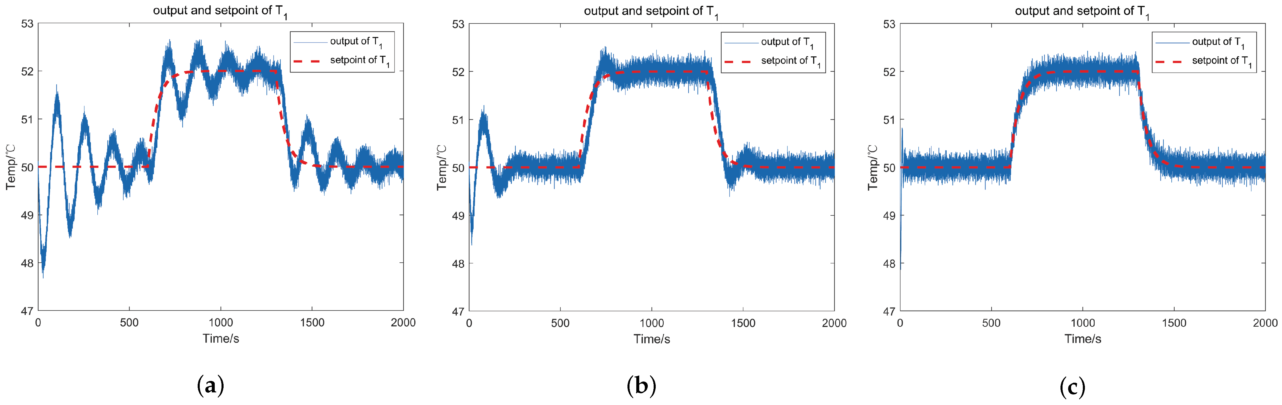
The outputs and setpoints of $T_1$ under various control frameworks are presented in Figure 4. It is evident that the outputs of $T_1$ exhibit inadequate setpoint tracking performance under the SPC framework. The output curves show erratic behavior, characterized by shaking and oscillations, making the tracking of setpoints ineffective during set point changes. Conversely, the tracking performance under the ASPC framework improves, effectively following setpoints after a settling time. However, during the setpoint of $T_1$ transitions, the tracking performance diminishes, leading to overshooting and less accurate setpoint tracking. The tracking performance under the proposed NSPC-LWPR framework shows the most promising results among the three control approaches. Even when the setpoints of $T_1$ change at 600 s and 1300 s, the $T_1$ outputs consistently track the setpoints.

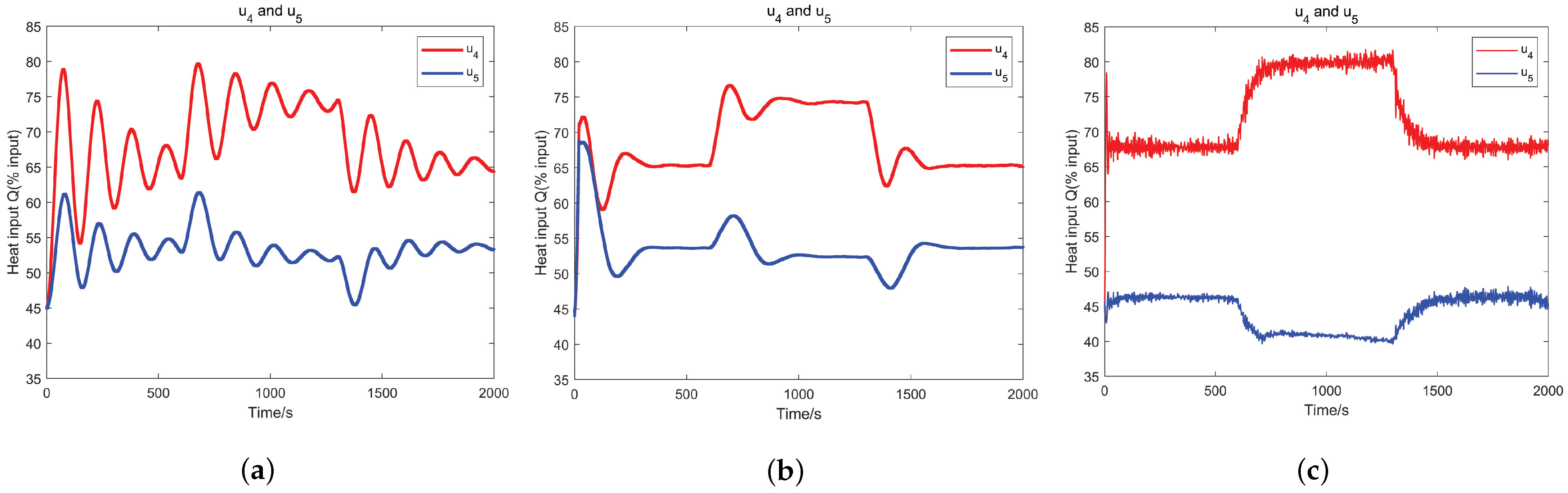
The disparities observed in the tracking performance of $T_1$ can be attributed to variations in the subspace predictor outputs generated by the controllers under different control frameworks as illustrated in Figure 5. The SPC method employs a fixed, offline-designed subspace predictor, making it unsuitable for effectively controlling nonlinear systems. In contrast, the ASPC method incorporates online learning capabilities to optimize its parameters based on process data, enabling it to adapt to changing conditions and generate corresponding subspace predictor outputs dynamically. However, the ASPC method remains linear and approximates new conditions using fixed nearby sampling points. Consequently, this approach can lead to degraded tracking performance and overshooting issues during smooth setpoint changes. Similar to the ASPC method, the proposed NSPC-LWPR approach is equipped with autonomous learning capabilities, allowing real-time updates of controller information using newly generated process data. However, it surpasses the limitations of the ASPC controller by employing multiple linear working points for weighted summation. This innovative approach constructs a nonlinear subspace predictive controller, leading to a more precise predictive output for the current operating condition.

The results indicate that the proposed NSPC-LWPR approach excels in describing the current nonlinear operating condition and achieves superior tracking performance in nonlinear industrial process control compared to SPC and ASPC methods. This highlights its potential as an advanced and effective controller in nonlinear industrial process system applications.

According to Figure 4 and Figure 5, the outputs of the controlled system and subspace predictor are strictly limited within specific boundaries. Additionally, the change rates of $u_4$ and $u_5$ are investigated and shown in Figure 6. It can be observed that the values of $\Delta u_4$ and $\Delta u_5$ both fall within the range of −0.5 and 0.5, which aligns with the constraints set. This result indicates that the proposed NSPC-LWPR approach operates within the imposed constraints, which effectively influence the system behavior.

To demonstrate the predictive performance of the proposed NSPC-LWPR approach, we conduct a comparative analysis using the multi-step prediction means squared error (MPMSE), defined as:

$$\sigma \left(N_p\right)=\sum _{k=T_s}^{T_t}\sum _{j=1}^{N_p}{∥\widehat{y}\left(k+j\right)-y\left(k+j\right)∥}^2/\left(N·N_p\right),$$

(37)

where $T_s$ and $T_t$ represent the starting point and the terminal point of the sampling data considered for analysis. To account for the necessary initialization time required by the proposed NSPC-LWPR approach, we set $T_s$ to be 400, and $T_t$ to be 10,000. The multi-step prediction mean squared error comparison among different control algorithms with varying predictive horizon $N_p$ is presented in

Table 6. Multi-step prediction mean squared error (MPMSE) comparison.

Control Methods	${\mathit{N}}_{\mathit{p}}=3$	${\mathit{N}}_{\mathit{p}}=4$	${\mathit{N}}_{\mathit{p}}=5$	${\mathit{N}}_{\mathit{p}}=6$	${\mathit{N}}_{\mathit{p}}=7$
SPC	1.5429	1.2649	1.0923	0.9732	0.8983
ASPC	0.1321	0.1147	0.1026	0.0934	0.0896
NSPC-LWPR	0.0946	0.0845	0.0740	0.0711	0.0661

.

Table 6 reveals a clear trend in the MPMSE, where the proposed NSPC-LWPR approach consistently outperforms the ASPC method and significantly outpaces the SPC method, all while maintaining a constant value of $N_p$. This performance discrepancy can be attributed to the SPC method’s limited ability to effectively control nonlinear systems, leading to subpar output predictions. In contrast, both the ASPC and NSPC-LWPR approaches exhibit self-learning capabilities, enhancing their control of nonlinear systems. However, the proposed NSPC-LWPR approach stands out by demonstrating superior predictive accuracy under the current operational conditions.

Furthermore, as $N_p$ increases, MPMSE decreases across all three methods. This decline is attributed to the broader prediction range, resulting in higher prediction accuracy. The outcomes of this comparative analysis compellingly support the superiority of the proposed NSPC-LWPR approach in terms of predictive performance. This finding indirectly substantiates its efficacy in enhancing tracking capabilities, underscoring its potential for effective control in nonlinear industrial process systems.

In total, data analysis in this study was conducted using Python programming language (V3.9.2) with the following libraries: NumPy (V1.21.6), SciPy (V1.11.0), and Matplotlib (V3.3.1) [36].

5. Conclusions

In this paper, we propose a NSPC-LWPR approach to address tracking issues in nonlinear industrial process control. Our approach integrates the LWPR algorithm into the framework of the SPC method, harnessing the exceptional nonlinear handling capabilities of LWPR. Through the segmentation of the input space into localized regions, the construction of precise local models, and their aggregation through weighted summation, our approach adeptly captures dynamic system characteristics and trains the regression model. The adaptability and efficiency of our approach are further augmented by a dynamic control strategy that adjusts based on the online process data and the parameters of established local models. Furthermore, the verification of our approach against the CSTH benchmark unequivocally demonstrates its superiority over conventional SPC and ASPC methods. This verification affirms its ability to significantly enhance tracking precision and predictive accuracy in industrial process control.

While our proposed control approach has demonstrated exceptional performance, it is important to acknowledge that there remain unexplored avenues for further research. Future investigations could delve into methodological refinements, expanding the applicability of our approach to diverse control problems, or exploring advanced variants of the LWPR algorithm.

References

- Dong, Y.; Lang, Z.Q.; Zhao, J.; Wang, W.; Lan, Z. A Novel Data-Driven Approach to Analysis and Optimal Design of Forced Periodic Operation of Chemical Reactions. IEEE Trans. Ind. Electron. 2023, 70, 8365–8376. [Google Scholar] [CrossRef]
- Wen, S.; Guo, G. Distributed Trajectory Optimization and Sliding Mode Control of Heterogenous Vehicular Platoons. IEEE Trans. Intell. Transp. Syst. 2022, 23, 7096–7111. [Google Scholar] [CrossRef]
- Du, S.; Wu, M.; Chen, X.; Cao, W. An Intelligent Control Strategy for Iron Ore Sintering Ignition Process Based on the Prediction of Ignition Temperature. IEEE Trans. Ind. Electron. 2020, 67, 1233–1241. [Google Scholar] [CrossRef]
- Li, S.; Zheng, Y.; Li, S.; Huang, M. Data-Driven Modeling and Operation Optimization with Inherent Feature Extraction for Complex Industrial Processes. IEEE Trans. Autom. Sci. Eng. 2023, 21, 1092–1106. [Google Scholar] [CrossRef]
- Zhou, P.; Zhang, S.; Wen, L.; Fu, J.; Chai, T.; Wang, H. Kalman Filter-Based Data-Driven Robust Model-Free Adaptive Predictive Control of a Complicated Industrial Process. IEEE Trans. Autom. Sci. Eng. 2022, 19, 788–803. [Google Scholar] [CrossRef]
- Ren, L.; Meng, Z.; Wang, X.; Zhang, L.; Yang, L.T. A Data-Driven Approach of Product Quality Prediction for Complex Production Systems. IEEE Trans. Ind. Inform. 2021, 17, 6457–6465. [Google Scholar] [CrossRef]
- Harbaoui, H.; Khalfallah, S. An Effective Optimization Approach to Minimize Waste in a Complex Industrial System. IEEE Access 2022, 10, 13997–14012. [Google Scholar] [CrossRef]
- Mehrtash, M.; Capitanescu, F.; Heiselberg, P.K.; Gibon, T. A New Bi-Objective Approach for Optimal Sizing of Electrical and Thermal Devices in Zero Energy Buildings Considering Environmental Impacts. IEEE Trans. Sustain. Energy 2021, 12, 886–896. [Google Scholar] [CrossRef]
- Zhang, F.; Kodituwakku, H.A.D.E.; Hines, J.W.; Coble, J. Multilayer Data-Driven Cyber-Attack Detection System for Industrial Control Systems Based on Network, System, and Process Data. IEEE Trans. Ind. Inform. 2019, 15, 4362–4369. [Google Scholar] [CrossRef]
- Kang, E.; Qiao, H.; Chen, Z.; Gao, J. Tracking of Uncertain Robotic Manipulators Using Event-Triggered Model Predictive Control With Learning Terminal Cost. IEEE Trans. Autom. Sci. Eng. 2022, 19, 2801–2815. [Google Scholar] [CrossRef]
- Choi, W.Y.; Lee, S.H.; Chung, C.C. Horizonwise Model-Predictive Control With Application to Autonomous Driving Vehicle. IEEE Trans. Ind. Inform. 2022, 18, 6940–6949. [Google Scholar] [CrossRef]
- Oshnoei, A.; Kheradmandi, M.; Khezri, R.; Mahmoudi, A. Robust Model Predictive Control of Gate-Controlled Series Capacitor for LFC of Power Systems. IEEE Trans. Ind. Inform. 2021, 17, 4766–4776. [Google Scholar] [CrossRef]
- Shang, C.; You, F. A data-driven robust optimization approach to scenario-based stochastic model predictive control. J. Process Control 2019, 75, 24–39. [Google Scholar] [CrossRef]
- Yao, L.; Shao, W.; Ge, Z. Hierarchical Quality Monitoring for Large-Scale Industrial Plants With Big Process Data. IEEE Trans. Neural Netw. Learn. Syst. 2021, 32, 3330–3341. [Google Scholar] [CrossRef] [PubMed]
- Han, H.; Fu, S.; Sun, H.; Qiao, J. Data-Driven Multimodel Predictive Control for Multirate Sampled-Data Nonlinear Systems. IEEE Trans. Autom. Sci. Eng. 2023, 20, 2182–2194. [Google Scholar] [CrossRef]
- Habib, M.; Wang, Z.; Qiu, S.; Zhao, H.; Murthy, A.S. Machine Learning Based Healthcare System for Investigating the Association Between Depression and Quality of Life. IEEE J. Biomed. Health Inform. 2022, 26, 2008–2019. [Google Scholar] [CrossRef]
- Sun, Q.; Ge, Z. A Survey on Deep Learning for Data-Driven Soft Sensors. IEEE Trans. Ind. Inform. 2021, 17, 5853–5866. [Google Scholar] [CrossRef]
- Xue, W.; Fan, J.; Lopez, V.G.; Li, J.; Jiang, Y.; Chai, T.; Lewis, F.L. New Methods for Optimal Operational Control of Industrial Processes Using Reinforcement Learning on Two Time Scales. IEEE Trans. Ind. Inform. 2020, 16, 3085–3099. [Google Scholar] [CrossRef]
- Kadali, R.; Huang, B.; Rossiter, A. A data driven subspace approach to predictive controller design. Control Eng. Pract. 2003, 11, 261–278. [Google Scholar] [CrossRef]
- Li, Z.; Wang, H.; Fang, Q.; Wang, Y. A data-driven subspace predictive control method for air-cooled data center thermal modelling and optimization. J. Frankl. Inst. 2023, 360, 3657–3676. [Google Scholar] [CrossRef]
- Navalkar, S.T.; van Solingen, E.; van Wingerden, J.W. Wind Tunnel Testing of Subspace Predictive Repetitive Control for Variable Pitch Wind Turbines. IEEE Trans. Control Syst. Technol. 2015, 23, 2101–2116. [Google Scholar] [CrossRef]
- Zhang, X.; Zhang, L.; Zhang, Y. Model Predictive Current Control for PMSM Drives With Parameter Robustness Improvement. IEEE Trans. Power Electron. 2019, 34, 1645–1657. [Google Scholar] [CrossRef]
- Wahab, N.A.; Katebi, R.; Balderud, J.; Rahmat, M.F. Data-driven adaptive model-based predictive control with application in wastewater systems. Control Theory Appl. IET 2010, 5, 803–812. [Google Scholar] [CrossRef]
- Vajpayee, V.; Mukhopadhyay, S.; Tiwari, A.P. Data-Driven Subspace Predictive Control of a Nuclear Reactor. IEEE Trans. Nucl. Sci. 2018, 65, 666–679. [Google Scholar] [CrossRef]
- Hallouzi, R.; Verhaegen, M. Fault-Tolerant Subspace Predictive Control Applied to a Boeing 747 Model. J. Guid. Control Dyn. 2008, 31, 873–883. [Google Scholar] [CrossRef]
- Zhou, P.; Zhang, S.; Dai, P. Recursive Learning-Based Bilinear Subspace Identification for Online Modeling and Predictive Control of a Complicated Industrial Process. IEEE Access 2020, 8, 62531–62541. [Google Scholar] [CrossRef]
- Zhou, P.; Song, H.; Wang, H.; Chai, T. Data-Driven Nonlinear Subspace Modeling for Prediction and Control of Molten Iron Quality Indices in Blast Furnace Ironmaking. IEEE Trans. Control Syst. Technol. 2017, 25, 1761–1774. [Google Scholar] [CrossRef]
- Luo, X.S.; Song, Y.D. Data-driven predictive control of Hammerstein–Wiener systems based on subspace identification. Inf. Sci. 2018, 422, 447–461. [Google Scholar] [CrossRef]
- Vijayakumar, S.; D’Souza, A.; Schaal, S. Incremental Online Learning in High Dimensions. Neural Comput. 2006, 17, 2602–2634. [Google Scholar] [CrossRef]
- Ferranti, F.; Rolain, Y. A local identification method for linear parameter-varying systems based on interpolation of state-space matrices and least-squares approximation. Mech. Syst. Signal Process. 2017, 82, 478–489. [Google Scholar] [CrossRef]
- De Caigny, J.; Camino, J.F.; Swevers, J. Interpolating model identification for SISO linear parameter-varying systems. Mech. Syst. Signal Process. 2009, 23, 2395–2417. [Google Scholar] [CrossRef]
- Felici, F.; van Wingerden, J.W.; Verhaegen, M. Subspace identification of MIMO LPV systems using a periodic scheduling sequence. Automatica 2007, 43, 1684–1697. [Google Scholar] [CrossRef]
- Favoreel, W.; Moor, B.D.; Gevers, M. SPC: Subspace Predictive Control. IFAC Proc. Vol. 1999, 32, 4004–4009. [Google Scholar] [CrossRef]
- Atkeson, C.G.; Schaal, M.S. Locally Weighted Learning. Artif. Intell. Rev. 1997, 11, 11–73. [Google Scholar] [CrossRef]
- Thornhill, N.F.; Patwardhan, S.C.; Shah, S.L. A continuous stirred tank heater simulation model with applications. J. Process Control 2008, 18, 347–360. [Google Scholar] [CrossRef]
- Johansson, R. Numerical Python: Scientific Computing and Data Science Applications with Numpy, SciPy and Matplotlib; Apress: New York, NY, USA, 2019. [Google Scholar]
Figure 1.
Information processing unit of the LWPR learning scheme.
Figure 2.
The control diagram of the proposed nonlinear subspace predictive control approach based on locally weighted projection regression (NSPC-LWPR) approach.
Figure 3.
The continuous stirred tank heater (CSTH) system in IIT Bombay.
Figure 4.
The outputs and setpoints of under different control frameworks. (a) Under the subspace predictive control (SPC) framework. (b) Under the adaptive subspace predictive control (ASPC) framework. (c) Under the NSPC-LWPR framework.
Figure 5.
Subspace predictor outputs and under different control frameworks. (a) Under the SPC framework. (b) Under the ASPC framework. (c) Under the NSPC-LWPR framework.
Figure 6.
Change rates of and .