Research on Dynamic Reactive Power Cost Optimization in Power Systems with DFIG Wind Farms

Abstract

As the power market system gradually perfects, the increasingly fierce competition not only drives industry development but also brings new challenges. Reactive power optimization is crucial for maintaining stable power grid operation and improving energy efficiency. However, the implementation of plant–grid separation policies has kept optimization costs high, affecting the profit distribution between power generation companies and grid companies. Therefore, researching how to effectively reduce reactive power optimization costs, both technically and strategically, is not only vital for the economic operation of the power system but also key to balancing interests among all parties and promoting the healthy development of the power market. Initially, the study analyzes and compares the characteristic curves of synchronous generators and DFIGs, establishes a reactive power pricing model for generators, and considering the randomness and volatility of wind energy, establishes a DFIG reactive power pricing model. The objective functions aimed to minimize the cost of reactive power purchased by generators, the price of active power network losses, the total deviation of node voltages, and the depreciation costs of discrete variable actions, thereby establishing a dynamic reactive power optimization model for power systems including doubly-fed wind farms. By introducing Logistic chaotic mapping, the CSA is improved by using the highly stochastic characteristics of chaotic systems, which is known as the Chaotic Cuckooing Algorithm. Meanwhile, the basic cuckoo search algorithm was improved in terms of adaptive adjustment strategies and global convergence guidance strategies, resulting in an enhanced cuckoo search algorithm to solve the established dynamic reactive power optimization model, improving global search capability and convergence speed. Finally, using the IEEE 30-bus system as an example and applying the improved chaotic cuckoo search algorithm for solution, simulation results show that the proposed reactive power optimization model and method can reduce reactive power costs and the number of discrete device actions, demonstrating effectiveness and adaptability. When the improved chaotic cuckoo algorithm is applied to optimize the objective function, the optimization result is better than 7.26% compared to the standard cuckoo search algorithm, and it is also improved compared to both the PSO algorithm and the GWO algorithm.

1. Introduction

As China’s economy advances with high quality on its development path, the demand for electricity from urban and rural residents and all sectors is increasing, making traditional energy sources insufficient to meet diverse needs. Currently, with the global rise in fossil fuel prices and the increasing dependence on traditional fuels by countries, wind power has come into focus and has rapidly developed against the backdrop of peak carbon and carbon neutrality goals. The rapid development of new energy sources has heralded the advent of green and low-consumption power generation. However, with the expansion of the power system’s scale and the increased demands for its functionality and maintenance, the complexities faced by the system have also intensified. Due to the inherent distributed nature, randomness, and uncertainty of wind energy, and under the influence of meteorological and environmental conditions, the reliability of its power supply is significantly reduced compared to conventional power generation methods. The intermittent and stochastic output of wind turbine generators presents an additional challenge to the stability of grid operations. Particularly, the introduction of various reactive power compensation devices and distributed energy sources has led to issues that compromise system safety and power quality, such as insufficient reactive power, increased network losses, severe voltage deviations, and deteriorated power quality. In light of this, to ensure the safe and economical operation of the power system, efforts must be made to balance the distribution of reactive power as evenly as possible throughout the system and to maintain the stability of grid voltage, thereby safeguarding the power quality for end-users.

In recent years, the Doubly-Fed Induction Generator (DFIG) has become the preferred choice for widespread application in the wind power generation sector. This type of generator not only allows for the adjustment of active and reactive power but also exhibits significant cost advantages due to its ease of installation and cost-effectiveness compared to other types of generators. Therefore, it is anticipated that the application of DFIGs in power systems will become even more widespread, having already captured a major market share in the wind turbine market. The Doubly-Fed Induction Generator (DFIG) can utilize power electronics technology to achieve decoupled control of active and reactive power. Due to the low power density characteristic of wind power generation, wind turbine generators spend most of their time operating under light-load conditions. Under such light-load conditions, the DFIG demonstrates a certain potential for reactive power output. Existing references [1,2] have explored the role of wind farms with DFIGs in reactive power optimization regulation within strong grid environments, particularly emphasizing the importance of employing local compensation principles for reactive compensation in wind farms containing DFIGs. To fully leverage the reactive power regulation capacity brought about by the integration of wind farms into the grid, considerations were also made for the principles of reactive power distribution among the turbines within the wind farm, as well as the reactive power optimization regulation between the stator of each wind turbine generator and the grid-side converter; ref. [3] engages wind farms with DFIGs connected to the network as continuous reactive power sources to participate in reactive power optimization, serving a reactive support role. It established a reactive optimization model with the objective function of minimizing the sum of active power network losses and node voltage deviations, taking into account safety indicators, transforming the reactive power optimization problem of the distribution network into a multi-constrained nonlinear mathematical problem, and solving the established model using the Particle Swarm Optimization (PSO) algorithm; ref. [4] targets the characteristics of wind farm grid connection and wind speed variability, applies the Q–U power flow calculation method, and constructs a multi-objective reactive power optimization model aimed at minimizing system active power losses, minimizing voltage deviations, and maximizing static voltage stability margins. Ref. [5], considering the reactive power regulation capability of DFIGs, establishes an operating steady-state model of the distribution network with variable-speed, constant-frequency wind turbine units. It calculates the power distribution on the stator and rotor sides of the unit based on the power curve and proposes how to determine the reactive power capacity limits of the DFIG. Applied to voltage analysis, it can effectively reduce active network losses and stabilize node voltages. Refs. [6,7] propose an improved Differential Evolution algorithm based on traditional evolutionary algorithms, effectively solving the reactive power optimization problem and demonstrating good adaptability and efficiency. Ref. [8] introduces a reactive power distribution strategy for DFIG, which considers not only the losses in transmission lines but also the losses during the internal energy conversion process within wind power generators. The aforementioned studies, while discussing reactive power optimization in power systems, primarily focus on minimizing system active power losses and optimizing voltage stability margins, without delving into the issue of reactive power costs within the context of the electricity market.

In the context of promoting fair competition in the electricity market, a notice on the reform plan for the electricity system issued by the State Council in 2002 introduced a strategy of separating generation and transmission in China’s energy management system, meaning that different power plants would belong to different generation groups. To reduce operational costs, these companies are usually reluctant to have their generating units produce additional reactive power, as this could not only shorten the lifespan of the units but also lead to increased costs due to the reduction in active power output caused by the additional reactive power generation. Despite this, the practice of generation companies reducing reactive power output could cause economic losses to the grid and carry the risk of operational quality not meeting standards. Therefore, to balance the interests of grid operation and generation companies, when generation companies incur losses due to increased reactive power output, grid companies should provide appropriate economic compensation to the generation companies. This study analyzes the DFIG pricing model considering wind speed fluctuations, based on the synchronous generator model established in references [9,10].

Ref. [11] proposed a microgrid demand response configuration method based on adaptive chaotic improved NSGA-II, which introduced chaotic sequences and adaptive strategies into the traditional NSGA-II and used a normally distributed crossover operator as well as a dynamic updating operator, and verified the effectiveness of the improved algorithm by comparing it with the MOPSO algorithm. Ref. [12] established a model of AC microgrid in grid-connected mode, and introduced the nonlinear convergence factor into the original grey wolf algorithm, which can effectively improve the daily operation economic efficiency of microgrid, but the environmental pollution treatment cost was not considered in the paper. Ref. [13] proposed an efficient cuckoo search algorithm to solve the combined heat and power economic scheduling problem under the premise of satisfying the heat demand while considering the system power and other constraints, and verified that its improved algorithm to solve the optimal scheduling problem is effective and feasible. Ref. [14] proposed an improved cuckoo search algorithm based on reinforcement learning to solve the economic scheduling problem, while introducing techniques such as Gaussian stochastic wandering, quasi-pairwise learning, and adaptive discovery probability, and comparing it with other cuckoo variant algorithms to verify the superiority of the improved algorithm. Ref. [15] proposed a double cuckoo search algorithm based on dynamically adjusted probability, introducing techniques such as population distribution entropy and a new type of step factor, and experimental comparisons to verify the effectiveness of the improved algorithm. Ref. [16] found cuckoo algorithm search performance is poor, convergence speed is slow and other defects; the original algorithm of the dimension-by-dimension reverse learning to improve the convergence speed and search performance of the algorithm, and the improved algorithm and other cuckoo variant algorithms comparison, verify the effectiveness of the improved algorithm.

Compared with other intelligent algorithms, the cuckoo search algorithm [17] is suitable for solving power system optimization problems; the algorithm has the advantages of high robustness, fewer parameter settings, and a wide range of applicability, etc. The results of the study prove that the cuckoo search algorithm has a higher optimization performance than the genetic algorithm, firefly algorithm, and particle swarm algorithm [18], but there are still problems such as poor convergence accuracy due to the easy to fall into the local optimum when optimizing part of the multi-polar value function and other problems. Comparative results are shown in

Table 1. Intelligent algorithms gaps in research and comparison of strengths and weaknesses.

Algorithms	Cuckoo Search Algorithm (CSA)	Genetic Algorithm (GA)	Firefly Algorithm (FA)	Particle Swarm Algorithm (PSO)	Grey Wolf Optimization Algorithm (GWO)
Global search capability.	Efficient long-range exploration using Levy flights to enhance global search capability.	Dependent on crossover and mutation; may require more iterations to find global optimum.	Attraction mechanism may be limited by local search and difficult to find global optimum.	May be difficult to jump out of local optimum due to premature particle aggregation.	Swarm tracking and encircling prey strategies may be limited to a smaller search range in some cases.
Number of parameters.	Fewer parameters, mainly the probability of finding an exotic bird egg Pα; relatively simple tuning parameter.	Multiple parameters need to be adjusted, such as crossover rate, mutation rate, etc., and tuning is complex.	Attractor functions may need to be tuned to suit specific problems.	Parameters such as weights between individual best and global best solutions need to be carefully tuned.	More parameters, including wolf pack rank effects and tracking accuracy, require more careful parameter tuning.
Adaptability.	Simple rules and less parameter tuning make it easy to adapt to different types of optimization problems.	May perform better on some specific problems, but may not be as adaptable as CSA.	Performance under specific problems relies on tuning of attraction function.	Very effective for some problem types, but may require targeted parameter tuning to improve adaptability.	Specific social hierarchies and hunting strategies may have limitations in applicability and may require specific tuning for certain problems.
Avoiding early convergence.	Parasitic reproduction strategies and Levy flights are effective in avoiding premature convergence problems.	Premature convergence problems may be mitigated by appropriate strategies such as diversity maintenance.	Glow attraction mechanism helps diversity but may also encounter premature convergence problem.	Precocious convergence problems are easily encountered due to premature aggregation of particles at locally optimal solutions.	May still face the risk of premature convergence on high-dimensional complex problems despite the use of dynamics to reduce the distance between the wolf pack leader and the tracker.
Dynamic balance between exploration and exploitation.	Naturally balances dynamically between global exploration and local exploitation through algorithmic mechanisms.	Need to balance exploration and exploitation through crossover and mutation mechanisms.	Attraction mechanisms help balance exploration and exploitation, but the effect depends on parameter settings.	The ability to balance exploration and exploitation needs to be balanced by adjusting the relevant parameters.	Need to balance exploration and exploitation by adjusting the social hierarchy and behavior of wolves, which may not be efficient in some cases.

.

In the multi-objective reactive power optimization problem for power systems, the DIRECT algorithm [19] (DIviding RECTangles algorithm) is a global optimization algorithm that is mainly used to deal with continuous nonlinear multidimensional optimization problems. In power systems, it can be applied to reactive power optimization problems. The DIRECT algorithm divides the search space by splitting rectangles to ensure that the solution space is searched globally, which is conducive to finding better solutions [20]. However, for high-dimensional optimization problems or cases where the solution space is very large, its computational complexity and computational cost are high. And for problems with small local features in the solution space, a large number of iterations may be needed to reach convergence during the search process, and the algorithm converges slowly [21].

The Iterative Adaptive Efficient Partitioning Algorithm (EPA) [22] is an optimization algorithm used for solving complex problems when faced with a multi-objective reactive power optimization problem. The application of the EPA algorithm to multi-objective reactive power optimization can bring a number of advantages, and it is suitable for solving complex optimization problems [23]. However, the EPA algorithm may be affected by local optimal solutions, especially if the search space of the optimization problem is very complex or contains many local minima. For high-dimensional optimization problems or problems with complex constraints, the convergence may be slower and more iterations may be required to reach the desired solution. The performance of the DIRECT algorithm and the EPA algorithm is described above, but when faced with multi-objective optimization problems, high-dimensional problems, and problems containing locally optimal solutions, both algorithms show a decrease in convergence performance when compared to the cuckoo algorithm, and are not as applicable as the cuckoo algorithm, see

Table 2. Performance demonstration of DIRECT and EPA algorithms.

Algorithms	DIRECT Algorithm	EPA Algorithm
Global search capability.	For high-dimensional problems or problems containing a large number of local minima, there may still be a lack of search power. The DIRECT algorithm may require a higher number of iterations to cover the entire solution space.	The EPA algorithm requires more iterations to reach the global optimal solution when the solution space has a complex structure or there are multiple local optimal solutions.
Number of parameters.	In some cases, choosing appropriate parameter values can be challenging, especially for complex optimization problems and different application scenarios.	The EPA algorithm involves several parameters, such as population size, crossover probability, and variance probability. Selection of appropriate parameter values may be challenging.
Adaptability.	For problems with highly nonlinear or complex constraints. Due to its basic segmentation and evaluation strategy, the DIRECT algorithm may not be adequately adapted to the characteristics of these problems, leading to performance degradation.	For problems with complex constraints or nonlinear properties, the adaptation of the EPA algorithm may be less than optimal.
Avoiding early convergence.	For problems with a high degree of nonlinearity or peaks, the DIRECT algorithm may prematurely fall into local optima at the initial stage.	The EPA algorithm uses iterative optimization to progressively improve the solution and there is a low risk of premature convergence.
Dynamic balance between exploration and exploitation.	The DIRECT algorithm is relatively good at balancing the dynamics between exploration and exploitation.	EPA algorithms require a dynamic balance between exploration and exploitation to ensure that the right balance is found between global search and local optimization.

.

In summary, this study obtains the reactive power pricing model of synchronous generator and doubly-fed wind turbines by studying the output relationship between active and reactive power of the two generators. It also analyses the DFIG reactive power pricing model under fluctuation by segmenting the wind speed considering the existence of stochastic and fluctuating wind resources themselves, and establishes a dynamic reactive power optimization model of the power system under the electric power market under the constraints of satisfying the set objective function. This includes minimizing the active network loss cost of the system, minimizing the reactive power purchase cost, minimizing the depreciation cost of the number of operations of the discrete equipment, and minimizing the total deviation of the node voltage. In terms of zoning strategy, a wind power curve segmentation pricing method adapted to wind speed fluctuation is proposed. The proposed dynamic reactive power optimization model is solved by using an improved chaotic cuckoo search algorithm. The effectiveness and practicality of the proposed model and algorithm are verified by taking the IEEE30 node system as an example.

2. Reactive Power Pricing Model for Generators

In the process of power flow analysis and reactive power optimization, the utility company responsible for a given area needs to redistribute the reactive power generated within its own range of power plants to support the stability of the electrical system. This excessive burden of reactive power output may reduce the expected lifespan of generating units and increase the frequency of required maintenance, thereby leading to a direct increase in power plant costs. Therefore, grid companies should enhance the enthusiasm of generating companies to produce reactive power from a technical level, by compensating for the losses incurred by generating companies due to bearing an excessive portion of reactive power.

2.1. Reactive Power Pricing Model for Synchronous Generator

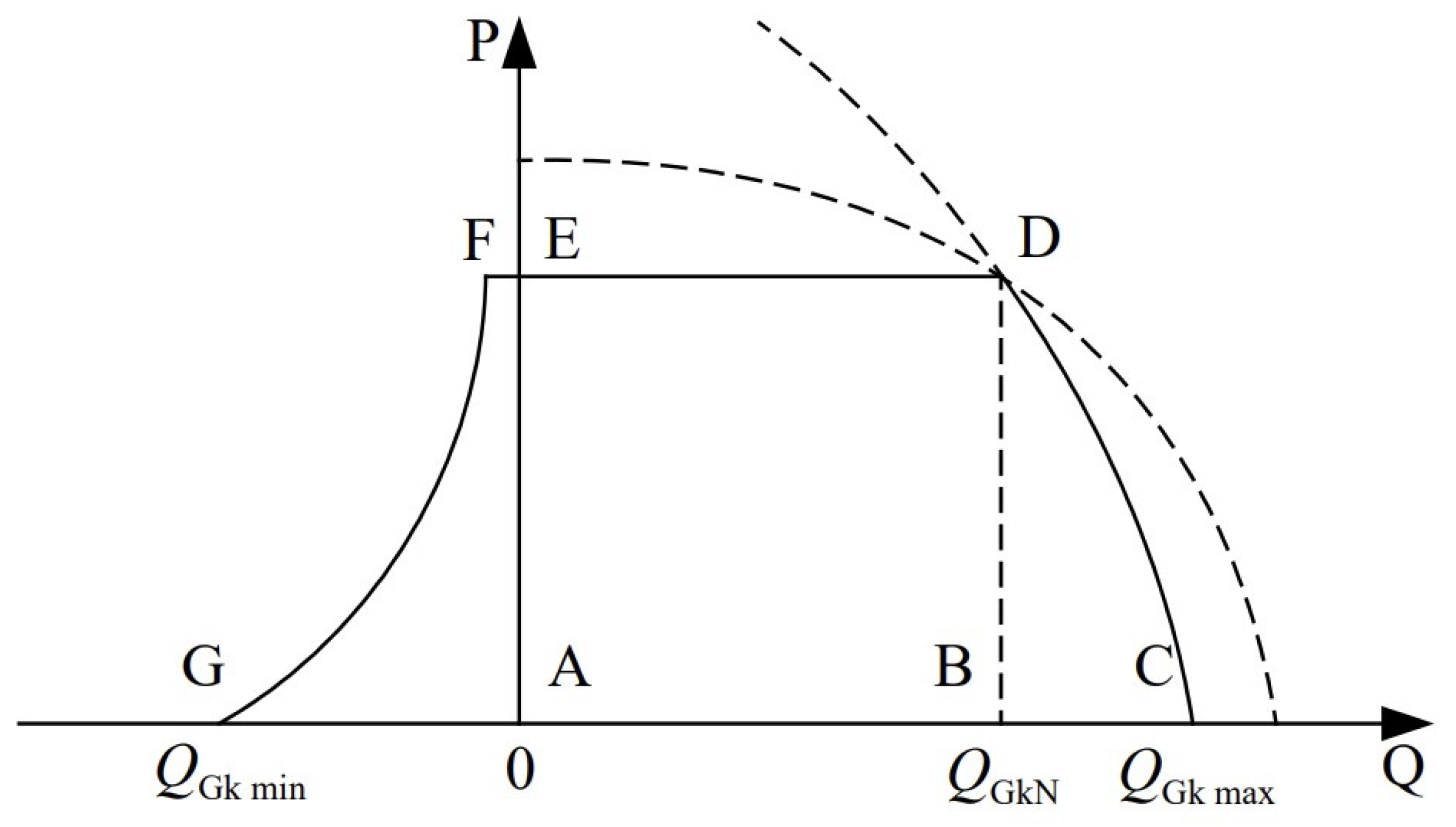
Based on the synchronous motor mathematical model constructed in refs. [24,25], the P-Q characteristics diagram of the synchronous motor is shown in Figure 1, with the GBDF area marked as the operating region of the motor. Based on pricing principles, this operating area is divided into three distinct regions:

In Region 1, the AEFG area in the diagram, it is observed that as the reactive power absorbed by the grid from the generating facilities increases, the maximum active power output correspondingly decreases. This phenomenon is accompanied by an increase in stator core temperature, reducing the expected lifespan of the generating units due to operation at high temperatures.

In Region 2, the ABDE area in the diagram, the output of reactive power leads to an increase in current, which accelerates the aging process of insulation materials, thereby increasing operational and maintenance costs. However, within this region, the impact of reactive power output on generation costs is relatively small.

In Region 3, the BCD area in the diagram, the curve shows that the maximum value of active power output decreases as reactive power output increases, resulting in a decrease in power factor.

To incentivize power plants to undertake more reactive power output, grid companies should proactively provide compensation to the relevant generating enterprises:

$$f_{\mathrm{QGm}}=\left\{\begin{array}{lll}\hspace{1em}\hspace{1em}{\lambda }_1\left|Q_{\mathrm{Gk}}\right|& & \hspace{1em}\hspace{1em}\hspace{1em}{Q}_{\mathrm{Gk}}\in \left[Q_{\mathrm{Gkmin}},0\right)\\ \hspace{1em}\hspace{1em} {\lambda }_2{Q}_{\mathrm{Gk}}& & \hspace{1em}\hspace{1em}\hspace{1em}{Q}_{\mathrm{Gk}}\in \left[0,Q_{\mathrm{GkN}}\right]\\ {\lambda }_2{Q}_{\mathrm{Gk}}+{\lambda }_{\mathrm{loss}}\mathsf{\Delta }{P}_{\mathrm{G}}& & \hspace{1em}\hspace{1em}\hspace{1em}{Q}_{\mathrm{Gk}}\in \left(Q_{\mathrm{GkN}},Q_{\mathrm{Gkmax}}\right]\end{array}\right.$$

(1)

In Equation (1), the reactive power price of a synchronous generator at the price boundaries of Region 1 and Region 2 is denoted by ${\lambda }_1$ and ${\lambda }_2$; the boundary price for the active power of the synchronous generator can be expressed as ${\lambda }_{loss}$; the reactive power output required from the generator under the dispatch of the grid company is denoted as $Q_{Gk}$; the maximum and minimum reactive power that can be generated by the synchronous generator within a reasonable output range are denoted by $Q_{\mathrm{Gkmax}}$ and $Q_{\mathrm{Gkmin}}$; the reduction in active power output due to the synchronous generator taking on additional reactive power is denoted by $\mathsf{\Delta }{P}_{\mathrm{G}}$; the reactive power output of the synchronous generator under rated conditions is denoted as $Q_{\mathrm{GkN}}$.

2.2. Reactive Power Pricing Model for DFIG (Doubly-Fed Induction Generators)

Most of the time, the grid-side converter operates at a unity power factor [26], and the reactive power emitted by the DFIG’s grid-side converter causes fluctuations in active power output [27]. Therefore, this study does not account for the reactive power emitted by the grid-side converter:

$$Q_T=Q_S$$

(2)

When DFIG operates in maximum power tracking mode:

$$P_T=K_{\mathrm{opt}}{(1-s)}^3$$

(3)

the influence of stator current on the reactive power limit of DFIG:

$$Q_T=\pm \sqrt{(3U_s{I}_s{)}^2-{(P/(1-s))}^2}$$

(4)

the impact of rotor current on the reactive power limit:

$$Q_T=-3\frac{U_s^2}{X_s}\pm \sqrt{{\left(3\frac{X_m}{X_s}{U}_s{I}_r\right)}^2-{\left(\frac{P_T}{1-s}\right)}^2}$$

(5)

In Equation (5), $Q_T$ represents the reactive power emitted by DFIG; $Q_S$ is the reactive power emitted by the stator side; $P_T$ is the active power output of the doubly-fed wind generator; $s$ is the slip rate; $K_{opt}$ is the maximum power tracking constant; $U_S$ is the stator voltage; $X_s$ and $X_m$ are respectively the stator reactance and the excitation reactance.

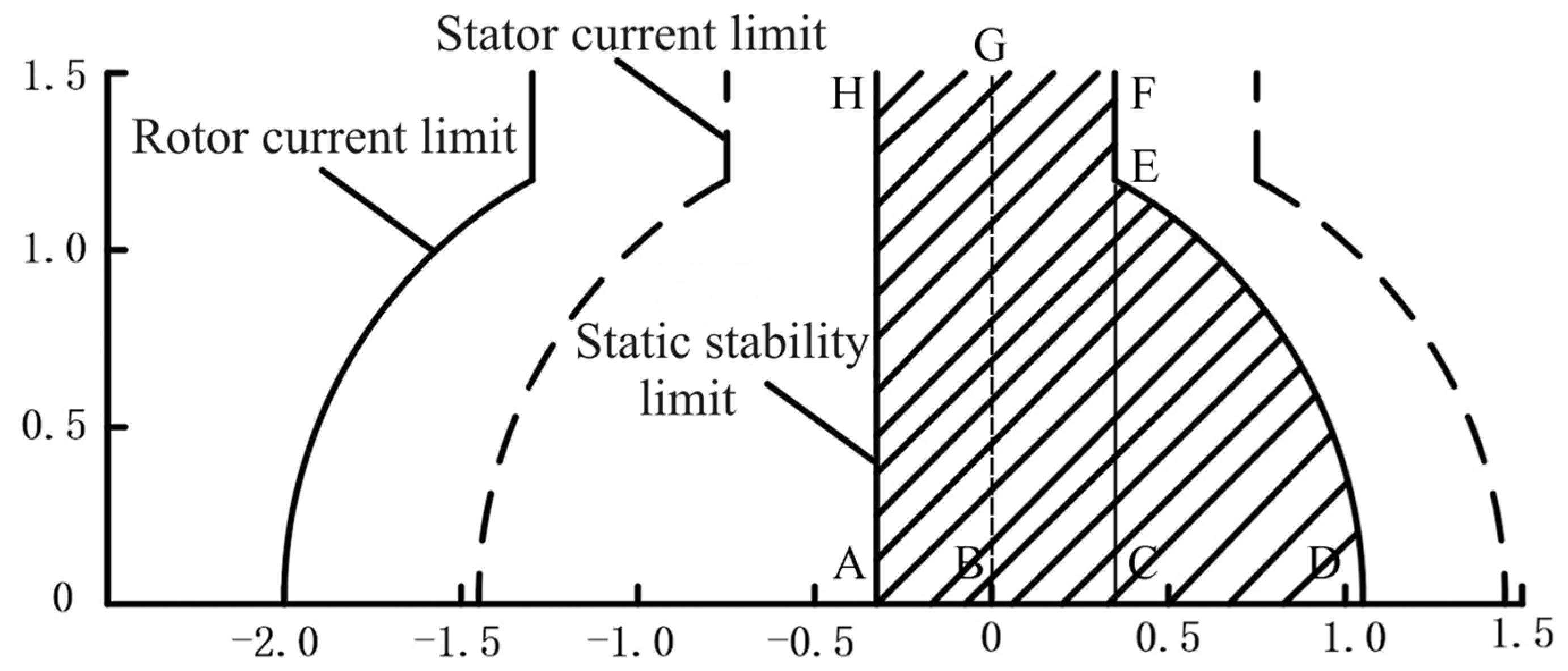
Referring to the unit model in ref. [28], the P-Q curve considering the static stability limit of DFIG is shown in Figure 2, where the shaded area represents the limit of reactive power output of the DFIG unit under different active power outputs.

The P-Q output relationship of doubly-fed wind generators is similar to that of synchronous generators, with reactive power pricing for the DFIG divided into three areas: Area ABGH, Area BCFG, and Area CDE, hereinafter referred to as Area 4, Area 5, and Area 6, respectively.

The compensation provided by the grid company to the generating companies should be as follows:

$$f_{\mathrm{QDm}}=\left\{\begin{array}{lll}{k}_1|Q_{\mathrm{T}}|& & \hspace{1em}\hspace{1em}\hspace{1em}{P}_{\mathrm{T}} Q_{\mathrm{T}}\in Area 4\\ k_2{Q}_{\mathrm{T}}& & \hspace{1em}\hspace{1em}\hspace{1em}{P}_{\mathrm{T}} Q_{\mathrm{T}}\in Area 5\\ k_2{Q}_{\mathrm{T}}+{\lambda }_{\mathrm{loss}}\mathsf{\Delta }{P}_D& & \hspace{1em}\hspace{1em}\hspace{1em}{P}_{\mathrm{T}} Q_{\mathrm{T}}\in Area 6\end{array}\right.$$

(6)

In Equation (6), which represents the marginal reactive power prices for Areas 1 and 2 of the DFIG, respectively, is the active power output reduced due to the increased emission of reactive power by the DFIG.

2.3. Reactive Power Pricing Model for DFIGs under Wind Speed Fluctuations

In the constructed dynamic reactive power optimization model, wind speeds within a 24 h period are segmented to capture real-time fluctuations in wind speed during the same time period. In this model, changes in wind speed during a specific period may lead to a situation where the doubly-fed induction generators (DFIGs) must reduce their active power output ($P_T$), in some cases due to excessive reactive power output ($Q_T$).

Specifically, assume that within a given wind speed range, there are regions where $n$ DFIGs need to adjust their active power output. For a particular DFIG, the region of reduced active power output can be represented by the shaded area in Figure 3. In this case, the average active power output when the DFIG operates in the region of reduced active power is defined as $P_M$, while the average active power output when the DFIG does not need to reduce active power to increase the reactive power it undertakes can be represented as $P_N$.

When operating in the area where active power output is reduced, the total reduction in active power is

$$\Delta W_D={\displaystyle \sum _{m=1}^n(P_N-P_m)}{t}_m$$

(7)

The reactive power price within a certain wind speed range is

$$f_{QD}=k_2{Q}_{T}t+{\lambda }_{\mathrm{loss}}\Delta W_D$$

(8)

In Equation (7), the time spent operating with reduced active power output due to reactive power distribution in the m-th segment is denoted by $t_m$; the cumulative operating time under this wind speed segment is denoted by $t$.

3. Dynamic Reactive Power Optimization Model for Power Systems with Doubly-Fed Wind Farms

The operation of discrete reactive power regulation equipment not only shortens the lifespan of the equipment itself but may also have adverse impacts on the entire power system [29,30]. Therefore, when constructing the objective function, in addition to minimizing the reactive power purchase cost of generators, the active power loss cost of the system, and the deviation of node voltage, the comprehensive cost of equipment also needs to be reduced to a certain target, namely minimizing the depreciation cost of operating discrete variables. This objective function employs the terminal voltage of synchronous machines, the reactive power output of DFIG units, the tap adjustments of on-load tap-changing transformers, and the capacity adjustments of grouped switched capacitors as control variables, thereby establishing a dynamic reactive power optimization model.

3.1. Wind Power Curve Segment Pricing Strategy

Given the inherently unstable fluctuations of wind resources, segmenting wind speed can mitigate the impact of volatility, and significantly reduce the operational costs of discrete devices. The entire process of wind farm fluctuations can be segmented, treating the fluctuating wind farm with a load segmentation strategy [31,32] and segmenting the fluctuating output curves, while employing the top-down algorithm [33] to solve the segmented wind power model.

The purpose of segmentation is to increase the disparity in average wind power output between different segments while reducing the variability of wind power output within the same segment, as described by the following mathematical model:

$$\left\{\begin{array}{l}{F}_1=\max {\displaystyle \sum _{i=1}^N}{\left(P_i-P\right)}^2\hfill \\ F_2=\min {\displaystyle \sum _{i=1}^N}{\displaystyle \sum _{j=1}^{K_i}}{\left(P_{ij}-P_i\right)}^2\hfill \end{array}\right.$$

(9)

In Equation (9), $N$ represents the number of wind speed segments; $K_i$ denotes the number of forecast points in the th segment; $P$ is the average forecasted wind speed over 24 h with 288 points for the wind farm; $P_i$ represents the average wind speed in the th segment; $P_{ij}$ indicates the value of the th point in the th wind speed segment.

To prevent the reduction of active power output due to excessive distribution of reactive power within each wind speed segment, the calculation of the reduction in active power output $\mathsf{\Delta }{W}_D$ for each wind turbine unit within a segment replaces the average wind power value with the maximum power point within the segment. This approach not only avoids reducing the unit’s active power output but also increases the reactive power margin of the generator set to a certain extent.

This means that for each wind turbine unit, when the reactive power output meets

$$Q_{\mathrm{DFIG}}>\sqrt{(3\frac{X_M}{X_S}{U}_S{I}_{\mathrm{R}\max }{)}^2-(\frac{P_{\mathrm{T}\max }}{1-s}{)}^2}$$

(10)

The reduction in active power output for each DFIG unit is calculated as

$$\Delta P_{\mathrm{Di}}=(1-s)\sqrt{(3\frac{X_M}{X_S}{U}_S{I}_{\mathrm{R}\max }{)}^2-(Q_{\mathrm{DFIG}}+3\frac{U_S^2}{X_S}{)}^2}$$

(11)

In Equation (11), $P_{T\max }$ represents the maximum active power output of each unit under this segment’s wind speed without reducing active output; $I_{R\max }$ is the maximum value of the rotor side current.

3.2. Objective Function

When constructing the multi-objective function, the following aspects were considered: minimizing the reactive power purchase cost of generators, reducing the cost of active power network losses, decreasing the depreciation expenses caused by the operation of discrete devices, and minimizing the total deviation of node voltages.

$$\left\{\begin{array}{l}{f}_1=\min \left({\lambda }_{\mathrm{loss}}{P}_{\mathrm{loss}}+\sum f_{\mathrm{QD}}+\sum f_{\mathrm{QG}}+\sum f_{\mathrm{Cq}}\right)\hfill \\ f_2=\min {\displaystyle \sum _{j=1}^n}\left|U_j-1\right|\hfill \end{array}\right.$$

(12)

In Equation (12), $P_{\mathrm{loss}}$ represents the active power network loss of the system; $\sum f_{\mathrm{QD}}$, $\sum f_{\mathrm{QG}}$, and $\sum f_{\mathrm{Cq}}$, respectively, represent the reactive power price of synchronous machines, DFIG units, and the depreciation cost of discrete device operations; $U_j$ is the voltage at node. After normalizing the objective function [34], the final objective function becomes

$$F_1=a_1{f}_1^{*}+a_2{f}_2^{*}$$

(13)

In Equation (13), $f_1^{*}$ and $f_2^{*}$ are the normalized objective functions; $a_1$ and $a_2$ are the weights of the objective functions calculated based on the Analytic Hierarchy Process (AHP) [35,36].

3.3. Constraint Conditions

(1)

Equality Constraints

The power flow calculation for each node’s equation power constraint conditions are given below:

$$\left\{\begin{array}{c}{P}_i=U_i{\displaystyle \sum _{j=1}^n{U}_j(G_{ij}\cos {\theta }_{ij}+B_{ij}\sin {\theta }_{ij})}+P_{\mathrm{L}i}\\ Q_i=U_i{\displaystyle \sum _{j=1}^n{U}_j(G_{ij}\sin {\theta }_{ij}-B_{ij}\cos {\theta }_{ij})+Q_{\mathrm{L}i}}\end{array}\right.$$

(14)

In Equation (14), the active and reactive power injected into the node are $P_i$ and $Q_i$, respectively; the active and reactive power loads injected into the $i$ node are $P_{Lj}$ and $Q_{Lj}$, respectively; the conductance and susceptance between $i$ node and $j$ node are $G_{ij}$ and $B_{ij}$, respectively; ${\theta }_{ij}$ is the voltage phase angle difference between $i$ node and $j$ node.

(2)

Inequality Constraints

The inequality constraints include the constraints on state variables and control variables:

$$\left\{\begin{array}{l}{P}_{\mathrm{g}i\min }\le P_{gi}\le P_{gi\max }\\ Q_{\mathrm{g}i\min }\le Q_{gi}\le Q_{gi\max }\\ U_{i\min }\le U_i\le U_{i\max }\\ P_{\mathrm{wfmin}}\le P_{\mathrm{wf}}\le P_{\mathrm{wf}\max }\\ Q_{\mathrm{wfmin}}\le Q_{\mathrm{wf}}\le Q_{\mathrm{wf}\max }\\ Q_{C_i\min }\le Q_{C_i}\le Q_{C_i\max }\\ {\displaystyle \sum _{t=1}^T{C}_i(t)\oplus C_i(t-1)\le n_{c\max }}\\ T_{i\min }\le T_i\le T_{i\max }\\ {\displaystyle \sum _{t=1}^T{T}_i(t)\oplus T_i(t-1)\le n_{t\max }}\end{array}\right.$$

(15)

In Equation (15), $P_{\mathrm{g}i\min }$ and $P_{\mathrm{g}i\max }$, respectively, denote the minimum and maximum active power output limits of the synchronous generator; $Q_{\mathrm{g}i\min }$ and $Q_{\mathrm{g}i\max }$ define the range of reactive power output; $U_{i\max }$ and $U_{i\min }$, respectively, represent the lowest and highest voltage limits at $i$ node. $P_{\mathrm{wf}\max }$ and $P_{\mathrm{wfmin}}$, $Q_{\mathrm{wf}\max }$ and $Q_{\mathrm{wfmin}}$, respectively, specify the limits on the active and reactive power outputs of the wind farm; the operational range of the shunt capacitor bank is denoted by $Q_{C_i\max }$ and $Q_{C_i\min }$; the upper and lower limits of the on-load tap changer position are given by $T_{i\max }$ and $T_{i\min }$; the capacities of the $i$ group of capacitors connected at times $t$ and $t-1$ are, respectively, represented by $C_i(t)$ and $C_i(t-1)$; $T_i(t)$ and $T_i(t-1)$, respectively, represent the tap positions of the $i$ transformer at times $T_i(t)$ and $T_i(t-1)$; the maximum number of switching operations for the capacitor bank and the maximum number of adjustments within reasonable capacity for transformer tap positions are represented by $n_{c\max }$ and $n_{t\max }$, respectively.

3.4. Handling of Constraint Conditions

In the extensive literature, the most widely used application for solving reactive power optimization problems is the penalty function method [37], a direct method that converts a multi-constraint optimization problem into an unconstrained optimization problem. The principle is that state variables that violate the constraints are considered infeasible solutions, and state variables that exceed the constraints in the objective function are “penalized” by the penalty function [38].

This paper addresses the issue of exceeding limits for control and state variables by superimposing a penalty function on the objective function, where the penalty function is defined as

$$G_{\mathrm{penalty}}=k_e\sum F(x)$$

(16)

In Equation (16), $k_e$ represents the penalty factor of the penalty function; $F(x)$ is

$$F(x)=\left\{\begin{array}{rrr}{(x-x_{\min })}^2& & x<x_{\min }\\ 0\hspace{1em}\hspace{1em} & & x_{\min }<x<x_{\max }\\ {\left(x-x_{\max }\right)}^2& & x>x_{\max }\end{array}\right.$$

(17)

$k_e$ is the penalty coefficient of the state variable, and $k_e$ is taken dynamically for better convergence of the objective function towards its minimum value.

A common approach is adaptive tuning, where the penalty coefficients are dynamically adjusted according to the current progress of the optimization process. For example, the size of the penalty coefficient can be adaptively adjusted according to the degree of constraint violation or the change in the value of the objective function. If the constraints are violated to a greater extent or the objective function value does not improve significantly, the penalty factor can be increased; on the contrary, if the constraints are satisfied or the objective function value improves, the penalty factor can be reduced.

$$k_e=k_{e\min }+K\times \frac{k_{e\max }-k_{e\min }}{K_{\max }}$$

(18)

In Equation (18), $K$ and $K_{\max }$ are the current iteration number and the maximum iteration number, respectively; $k_{e\max }$ and $k_{e\min }$ are the upper and lower limit values of the corresponding penalty coefficients, respectively. In order to obtain the minimum objective function value faster, the value of the penalty coefficient becomes larger with the increase in the number of iterations.

4. Reactive Power Optimization Based on Improved Chaotic Cuckoo Search Algorithm

The Cuckoo Search (CS) algorithm is a nature-inspired heuristic algorithm. Based on the parasitic brood behavior of cuckoos in nature, the CS algorithm stands out in global optimization due to its unique Levy flights and has shone in solving real-world engineering problems. It primarily relies on two strategies: cuckoo brood parasitism and Levy flight. This method is structurally simple, robust, highly adaptable, requires few parameters, and easily escapes local optima to avoid premature convergence.

The basic principle process is as follows: in the initial phase, the position parameters are updated through the random behavior strategy of Levy flights. Next, if the obtained random value exceeds the predefined discovery probability threshold, the system generates a new solution to replace the existing one based on random behavior of deviation. The formula for updating the nest position is

$$X_i^{k+1}=X_i^k+\alpha \oplus Levy(\lambda )$$

(19)

$$\alpha ={\alpha }_0\left(X_i^k-X_{\mathrm{best}}\right)$$

(20)

In Equations (19) and (20), $X_i^{k+1}$, $X_i^k$, and $X_{\mathrm{best}}$, respectively, represent the positions of the $i$ nest at the $k$, $k+1$ generation, and the current optimal position; $\alpha$ is the step-size control factor; ${\alpha }_0$ is a constant; $Levy(\lambda )$ is the path of Lévy random search.

$Levy(\lambda )$ follows a Lévy probability distribution:

$$Levy(\lambda )\sim u=t^{-\lambda }\hspace{1em}\hspace{1em}\hspace{1em}1<\lambda ⩽3$$

(21)

For computational convenience, the formula for calculating Lévy random numbers is given below:

$$Levy(\lambda )=\frac{\varphi u}{\left|\begin{array}{c}\nu \end{array}\right.{|}^{1/\lambda }}$$

(22)

when $u$, $v$ follow a standard normal distribution and $\lambda$ = 1.5:

$$\varphi ={\left\{\frac{\mathsf{\Gamma }(1+\lambda )\sin (\pi \lambda /2)}{\mathsf{\Gamma }\left\{2^{\frac{\lambda -1}{2}}\lambda \left[\frac{1+\lambda }{2}\right]\right\}}\right\}}^{1/\lambda }$$

(23)

Consequently, the update formula is derived:

$$X_i^{k+1}=X_i^k+{\alpha }_0\frac{\varphi u}{|v{|}^{1/\lambda }}\left(X_i^k-X_{\mathrm{best}}\right)$$

(24)

$$X_i^{k+1}=X_i^k+r\left(X_j-X_{\mathfrak{g}}\right)$$

(25)

In Equations (24) and (25), $X_{\mathrm{j}}$ and $X_{\mathrm{g}}$ are two random numbers of the current generation; $r$ is a scaling factor, a random number between [0, 1]. If the scaling factor exceeds the elimination probability, it is updated according to Equation (24).

In the standard CS algorithm, the highly random mechanism of Levy flights generates steps of varying lengths, leading to slow convergence speed and an inability to perform comprehensive global searches, making it prone to getting trapped in local optima. This study focuses on two crucial parameters that control the algorithm’s convergence speed: the step-size control factor $\alpha$ and the probability $P_a$ of being discovered by the host, proposing improvements for both.

Improvement 1: CSA generates the initial solution randomly in the feasible domain, which may cause the initial solution to fall into the local optimum directly, triggering premature growth. By introducing Logistic chaotic mapping, the CSA is improved by using the highly stochastic characteristics of chaotic systems, which is known as Chaotic Cuckooing Algorithm.

$$s=\frac{n_0-n_{0,\min }}{n_{0,\max }-n_{0,\min }}$$

(26)

$$S_1=\mu \times s\times (1-s)$$

(27)

$$n=n_{0,\min }+s_1(n_{0,\max }-n_{0,\min })$$

(28)

In Equations (26)–(28), $n_0$ is the randomly generated initial solution; $n_{0,\min }$ and $n_{0,\max }$ are the $n_0$ minimum and maximum values, respectively; $s$ and $S_1$ are the intermediate quantities generated by the chaotic mapping; $n$ is the logistic mapping processed solution; $\mu$ is the chaotic mapping parameter.

Improvement 2: an adaptive adjustment strategy is introduced for the step-size factor $\alpha$ and the probability $P_a$ of a cuckoo’s egg being discovered by the host in the host nest. In the iterative optimization of the basic CS algorithm, both better and worse solutions are processed with fixed $\alpha$ and $P_a$ values. When the $P_a$ value is too high and the $\alpha$ value relatively low, the optimization process may only achieve local optima prematurely without finding the global optimum. Conversely, if the $\alpha$ value is too low and the $P_a$ value too high, it may significantly slow down the optimization speed, thereby affecting the optimization performance. To address this issue, this study proposes an adaptive adjustment mechanism. During the optimization process, if an individual’s current fitness value (also known as the health value) is below the group’s average fitness, the $\alpha$ value will be dynamically adjusted; otherwise, if an individual’s value exceeds the group average, the maximum value replaces the current $\alpha$ value. This mechanism is also applicable to adjusting the $P_a$ value.

The specific expression is as follows:

$$\alpha =\left\{\begin{array}{lll}{\alpha }_{\min }+\frac{\left({\alpha }_{\max } - {\alpha }_{\min }\right)\left(fi{t}_i - fi{t}_{\min }\right)}{fi{t}_{mean} - fi{t}_{\min }}& & fi{t}_i\le fi{t}_{mean}\\ {\alpha }_{\max }& & fi{t}_i>fi{t}_{mean}\end{array}\right.$$

(29)

$$P_a=\left\{\begin{array}{lll}{P}_{a \min }+\frac{\left(P_{a\max } - P_{a\min }\right)\left(fi{t}_i - fi{t}_{\min }\right)}{fi{t}_{mean} - fi{t}_{\min }}& & fi{t}_i\le fi{t}_{mean}\\ P_{a\max }& & fi{t}_i>fi{t}_{mean}\end{array}\right.$$

(30)

In Equations (29) and (30), ${\alpha }_{\min }$ and ${\alpha }_{\max }$, respectively, signify the minimum and maximum constraint values for parameter $\alpha$; $fi{t}_{mean}$ and $fi{t}_{\min }$ represent the average fitness value of all feasible solutions in the current population and the lowest fitness value within the population, respectively; while $fi{t}_i$ indicates the current fitness value of a specific nest (as a potential solution) in the population.

Improvement 3: incorporating a global convergence guiding strategy into the search equation. When there is no record of the nest’s own optimum solution and the global optimum solution during the iteration process, a slowdown in convergence speed is observed, and the precision of the solution does not meet established requirements. To overcome this challenge, adopting the principles of the Particle Swarm Optimization (PSO) algorithm as a viable strategy aimed at enhancing the local exploration efficiency and speeding up the search process. In optimizing the Cuckoo Search (CS) algorithm, a set of improved optimization equations was developed by integrating Lévy flights with a global convergence guiding strategy.

$$x_i^{(k+1)}=v_i^{(k)}+H(u)\left(x_j^{(k)}-x_g^{(k)}\right)+H(u)\left(x_{pb}-x_i^{(k)}\right)+H(u)\left(x_{gb}-x_i^{(k)}\right)$$

(31)

In Equation (31), for the k-th generation, each nest has its optimum solution, $x_{pb}$, and the global optimum solution, $x_{gb}$, formed by all nests, is defined as the best solution for that generation; simultaneously, three randomly selected solutions. $x_i^{(k)}$, $x_j^{(k)}$, and $x_g^{(k)}$ are marked as the random solutions for that generation.

In the process of generating new solutions with Equation (31), by adopting a global convergence guiding strategy, the optimum solutions of each nest and the overall global optimum solution are recorded. This strategy uses the currently known optimum solutions as a guide, encouraging the algorithm to explore towards the direction of the global optimum solution. Moreover, this guiding mechanism promotes the process of individuals approaching the optimum individuals identified within the group, while also reducing the possibility of the algorithm getting trapped in local optima. Combined with Lévy flight random search, it significantly enhances the algorithm’s convergence efficiency.

The flowchart of the improved chaotic cuckoo search algorithm is shown in Figure 4.

5. Case Study Analysis

Taking the IEEE 30-bus system (as shown in Figure 5) as an example, simulation calculations are conducted to verify the effectiveness of the proposed strategies and algorithms, with system parameters referring to [39,40]. The system uses on-load tap-changing transformers with an adjustment range of ±6 taps and a tap ratio adjustment of 1% per tap. At nodes 26, 29, and 30, 10 groups of grouped switched shunt capacitors are connected, each with a capacity of 1 Mvar. The wind farm connected at node 7 consists of 50 1.5 MW doubly-fed wind turbines, with DFIG parameters seen in [41,42]. The wind farm does not consider wake effects or wind speed variations caused by geographical differences.

Generator operation information [43,44] is provided in

Table 3. Area of the generator operates.

Node	Area 1/Mvar	Area 2/Mvar	Area 3/Mvar
1	(−13.3, 0)	(0, 75)	(75, 100)
2, 5, 8	(−10, 0)	(0, 27)	(27, 36)
11, 13	(−7, 0)	(0, 18)	(18, 24)
7	(−12.4, 0)	(24.7, 0)	(24.7, 64.3)

; based on [45], the marginal reactive power price information is provided in

Table 4. Area of the generator operates.

Node Number	λ1 or k1 yuan/Mvar	λ2 or k2 yuan/Mvar
1	57.5	17.5
2, 5, 8, 11, 13	50	12.5
7	100	10

. The active power marginal price is set at 200 yuan/(MW·h), and the depreciation costs for grouped switched capacitors and on-load tap-changing transformers are 30 yuan/step and 40 yuan/step, respectively.

In this study, the wind power segmentation method is used to record data every 5 min within 24 h for the selected wind farm, totaling 288 points. The wind power forecast graph is divided into six sections, as seen in Figure 6.

In the first time period, reactive power optimization focuses on two objectives: minimizing network losses and minimizing node voltage deviation, while setting initial positions for discrete devices. From the second to the sixth time period, the objective function is expanded on the basis of the above two objectives and dynamic reactive power optimization is performed in

Table 5. Comparison of generator reactive power output.

Node	Objective Function 1 Reactive Power Output of Generators/Mvar	Objective Function 1 Reactive Power Output of Generators/Mvar	Objective Function 1 Reactive Power Output of Generators/Mvar
1	22.41	0.00	0.00
2	−1.68	8.14	6.23
5	19.19	0.02	0.74
7	8.59	38.31	30.73
8	35.07	4.08	16.34
11	1.01	4.27	1.48
13	−6.63	0.10	8.09

. The purpose of setting the first objective function is to minimize network losses and total voltage deviation of nodes as much as possible; based on the above two objectives, the objective function is expanded to include minimizing the reactive power costs of generators and network loss costs as the second objective function; based on the above objectives, a reasonable interval pricing strategy is proposed, taking into account the minimization of depreciation costs for discrete devices, forming the third objective function. In the fifth period, after the introduction of the reactive power pricing strategy, the second and third objective functions prioritize allocating more reactive resources to nodes with lower reactive costs, preventing generators from operating in a high-cost state of acquiring reactive power. During this period, the obtained average power and maximum power are 45.3 MW and 60.0 MW, respectively. In cases where an increase in reactive output causes a decrease in active output, the maximum achievable reactive outputs are 48.6 Mvar and 32.7 Mvar, respectively. The reduction in reactive power distribution for the third objective function is particularly notable at node 7. Supported by this pricing strategy, it can effectively reduce the increase in reactive power and the decrease in active power caused by fluctuations, achieving a reduction of 0.38 MWh.

The initial positions of the capacitors for Period 1 are determined by Objective Function 1, with changes in other positions shown in

Table 6. Capacitor gear comparison.

Time Period	Objective Function 1 Capacitor Stages C1, C2, C3	Objective Function 1 Capacitor Stages C1, C2, C3	Objective Function 1 Capacitor Stages C1, C2, C3
1	3, 2, 5
2	3, 2, 5	3, 2, 5	3, 2, 5
3	3, 2, 5	3, 2, 5	3, 2, 5
4	3, 2, 5	3, 2, 5	3, 2, 5
5	3, 2, 5	3, 2, 5	3, 2, 5
6	3, 2, 5	3, 2, 5	3, 2, 5

. For Periods 2 to 6, the simulation values from the previous period are utilized to obtain the simulation values for these periods, where C1, C2, and C3 represent the capacitor positions at nodes 26, 29, and 30, respectively. The number of transformer tap changes is shown in Figure 6. According to the data from Table 6 and Figure 7, it can be observed that Objective Function 1 has more frequent actions on discrete variables compared to other objective functions; a reduction in reactive power reserve can adversely affect system stability. The performance of Objective Function 2 is not conducive to system stability, as allocating too much reactive power to capacitors causes them to remain in high positions for extended periods, reducing reactive power reserve. Compared to Objective Function 2, Objective Function 3 has lower reactive power costs and better performance of reactive discrete devices. The adjustment frequency of capacitor positions is more active over longer periods, achieving better performance in terms of reactive power cost and the number of actions of discrete devices, with the position adjustments being appropriate. Compared with the two objective functions, the number of actions for Objective Function 3 decreased by 43.8% and 60.9%, respectively, and the number of transformer tap changes was reduced by 60.6% and 60.4%.

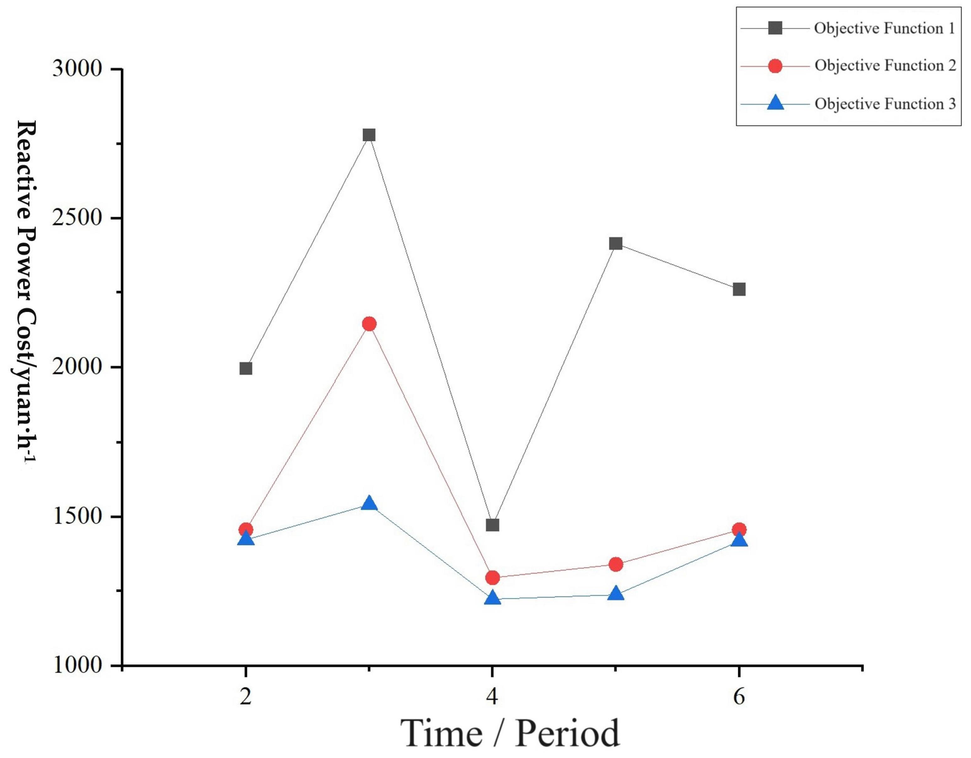
Figure 8 and Figure 9 show a comparative analysis of active network losses and reactive power costs. According to the data from Figure 7 and Figure 8, Objective Function 1 performs best in terms of network losses, but it has the highest reactive power costs. In contrast, Objective Function 2 has the highest network losses, but its reactive power costs are lower than the network losses of Objective Function 1. Objective Function 3 has the lowest reactive power costs compared to the other two, and Objective Function 2 has higher network losses than Objective Function 3, which in turn has more network losses than Objective Function 1. The reactive power cost of Objective Function 3 is 1183 yuan/h, which is 32.9% less than the 1764 yuan/h of Objective Function 1, and 4.6% less than the 1241 yuan/h of Objective Function 2. The results of the objective function analysis are shown in

Table 7. Analysis of the results of the objective function.

Optimization Term/Objective Function	Objective Function 3 versus Objective Function 2	Objective Function 3 versus Objective Function 1
Reduce the amount of active reduction due to increased reactive power.	Reduced by 0.38 MWh	Reduced by 0.82 MWh
Number of discrete equipment actions.	Reduced by 43.8 per cent	Reduced by 60.9 per cent
Number of transformer stall actions.	Reduced by 60.6 per cent	Reduced by 60.4 per cent
Cost of reactive power.	Reduced by 4.6 per cent	Reduced by 32.9 per cent

.

In the case analysis for period 2, the enhanced cuckoo search algorithm, the standard cuckoo search algorithm, and the particle swarm optimization algorithm were employed to solve the established model, with the iteration process displayed in Figure 10. As shown in Figure 10, it is evident that the enhanced cuckoo search algorithm significantly improved in terms of convergence speed and global search capability compared to the standard cuckoo search algorithm. When the enhanced cuckoo search algorithm is applied to optimize the objective function, the optimization results improved by 7.26% compared to the standard cuckoo search algorithm. It is also an improvement over the PSO algorithm, the GWO algorithm, the DIRECT algorithm, and the EPA algorithm.

6. Conclusions

This study proposes a reactive power pricing strategy in a zoning approach, considers reactive power costs, constructs a dynamic reactive power optimization model under constraint conditions, and applies an enhanced cuckoo search algorithm to solve the proposed model. The results indicate: (1) Compared to traditional models and static reactive power cost optimization models, the model developed in this study shows considerable advantages in optimizing reactive power cost prices and reducing the operation frequency of discrete devices, especially in reducing reactive power costs over longer periods. (2) The strategy of pricing based on segmented wind power output proposed in this study effectively prevents the reduction in active power output of units due to excessive reactive power output from doubly-fed induction generators (DFIG). (3) Solving the proposed reactive power optimization model with the enhanced cuckoo algorithm has significantly improved the model’s convergence speed and global optimization capability during the computation process, providing an effective and feasible method for addressing reactive power optimization issues.

References

- Soomro, M.; Memon, Z.A.; Baloch, M.H.; Mirjat, N.H.; Kumar, L.; Tran, Q.T.; Zizzo, G. Performance Improvement of Grid-Integrated Doubly Fed Induction Generator under Asymmetrical and Symmetrical Faults. Energies 2023, 16, 3350. [Google Scholar] [CrossRef]
- Huang, S.; Li, P.; Wu, Q.; Li, F.; Rong, F. ADMM-based distributed optimal reactive power control for loss minimization of DFIG-based wind farms. Int. J. Electr. Power Energy Syst. 2020, 118, 105827. [Google Scholar] [CrossRef]
- Zhou, S.; Rong, F.; Ning, X. Optimization Control Strategy for Large Doubly-Fed Induction Generator Wind Farm Based on Grouped Wind Turbine. Energies 2021, 14, 4848. [Google Scholar] [CrossRef]
- Wang, Z.; Zhang, L.; Li, G. The Active Power and Reactive Power Dispatch Plan of DFIG Based Wind Farm Considering Wind Power Curtailment. Int. J. Comput. Intell. Syst. 2015, 8, 553–560. [Google Scholar] [CrossRef]
- Li, B.; Zheng, D.; Li, B.; Jiao, X.; Hong, Q.; Ji, L. Analysis of low voltage ride-through capability and optimal control strategy of doubly-fed wind farms under symmetrical fault. Prot. Control. Mod. Power Syst. 2023, 8, 36. [Google Scholar] [CrossRef]
- Singh, S.P.; Prakash, T.; Singh, V.P. Coordinated tuning of controller-parameters using symbiotic organisms search algorithm for frequency regulation of multi-area wind integrated power system. Eng. Sci. Technol. Int. J. 2020, 23, 240–252. [Google Scholar] [CrossRef]
- Li, Y.; Li, X.; Li, Z. Reactive Power Optimization Using Hybrid CABC-DE Algorithm. Electr. Power Components Syst. 2017, 45, 980–989. [Google Scholar] [CrossRef]
- Meegahapola, L.; Perera, S. Capability constraints to mitigate voltage fluctuations from DFIG wind farms when delivering ancillary services to the network. Int. J. Electr. Power Energy Syst. 2014, 62, 152–162. [Google Scholar] [CrossRef]
- Meegahapola, L.; Durairaj, S.; Flynn, D.; Fox, B. Coordinated utilisation of wind farm reactive power capability for system loss optimisation. Eur. Trans. Electr. Power 2011, 21, 40–51. [Google Scholar] [CrossRef]
- Memon, A.; Bin Mustafa, M.W.; Jumani, T.A.; Obalowu, M.O.; Malik, N. Salp swarm algorithm–based optimal vector control scheme for dynamic response enhancement of brushless double-fed induction generator in a wind energy conversion system. Int. Trans. Electr. Energy Syst. 2021, 31, e13157. [Google Scholar] [CrossRef]
- Zhang, H.L.; Ouyang, T.; Yang, H.M. Demand Response Configuration of Microgrid Based on Adaptive Chaotic Improved NSGA-II. Control. Eng. China 2023, 30, 47–53. [Google Scholar]
- Gao, Y.; Huang, S.; Chen, L.X.; Huang, J. Economic optimization scheduling of grid-connected alternating current microgrid based on improved gray wolf algorithm. Sci. Technol. Eng. 2020, 20, 11605–11611. [Google Scholar]
- Nguyen, T.T.; Nguyen, T.T.; Vo, D.N. An effective cuckoo search algorithm for large-scale combined heat and power economic dispatch problem. Neural Comput. Appl. 2018, 30, 3545–3564. [Google Scholar] [CrossRef]
- Luo, W.G.; Yu, X.B. Reinforcement learning-based modified cuckoo search algorithm for economic dispatch problems. Knowl. Based Syst. 2022, 257, 109844. [Google Scholar] [CrossRef]
- Chen, C.; He, X.S.; Yang, X.S. Double Cuckoo Search Algorithm with Dynamically Adjusted Probability. J. Front. Comput. Sci. Technol. 2021, 15, 859–880. [Google Scholar]
- Huang, M.M.; He, Q.; Wen, X. Dynamically adaptive cuckoo search algorithm based on dimension by opposition-based learning. Appl. Res. Comput. 2020, 37, 1015–1019. [Google Scholar]
- Yang, X.S.; Deb, S. Cuckoo Search via Lévy Flights. In Proceedings of the 2009 World Congress on Nature & Biologically Inspired Computing, Coimbatore, India, 9–11 December 2009; IEEE: Piscataway, NJ, USA, 2009; pp. 210–214. [Google Scholar]
- Sun, M.; Wei, H. An improved cuckoo algorithm with adaptive inertia weight. J. Yangtze Univ. 2019, 16, 81–87. [Google Scholar]
- Wang, S.; Zhang, K.; Shi, D.; Li, M.; Yin, C. Research on economical shifting strategy for multi-gear and multi-mode parallel plug-in HEV based on DIRECT algorithm. Energy 2024, 286, 129574. [Google Scholar] [CrossRef]
- Finkel, D.E. DIRECT Optimization Algorithm User Guide; Center for Research in Scientific Computation, North Carolina State University: Raleigh, NC, USA, 2003. [Google Scholar]
- Jonesd, R.; Perttunenc, D.; Stuckmanb, E. Lipschitzian Optimization without the Lipschitz Constant. J. Optim. Theory Appl. 1993, 79, 157–181. [Google Scholar] [CrossRef]
- Jindal, P.; Pahuja, S. Swarm Algorithm-based Power Optimization in Cooperative Communication Network. Int. J. Sens. Wirel. Commun. Control 2023, 13, 285–295. [Google Scholar]
- Liping, D.; Ying, T.; Yiming, L.; Chen, Y. On the Energy Efficiency of Multicell Massive MIMO with Antenna Selection and Power Allocation. Wirel. Commun. Mob. Comput. 2022, 2022, 7224731. [Google Scholar]
- Roummani, K.; Hamouda, M.; Mazari, B.; Bendjebbar, M.; Koussa, K.; Ferroudji, F.; Necaibia, A. A new concept in direct-driven vertical axis wind energy conversion system under real wind speed with robust stator power control. Renew. Energy 2019, 143, 478–487. [Google Scholar] [CrossRef]
- Kassem, A.M.; Abdelaziz, A.Y. Firefly Optimization Algorithm for the Reactive Power Control of an Isolated Wind-Diesel System. Electr. Power Compon. Syst. 2017, 45, 1413–1425. [Google Scholar] [CrossRef]
- Cheng, Q.; Ma, X.; Cheng, Y. Coordinated Control of the DFIG Wind Power Generating System Based on Series Grid Side Converter and Passivity-Based Controller Under Unbalanced Grid Voltage Conditions. J. Electr. Eng. Technol. 2020, 15, 2133–2143. [Google Scholar] [CrossRef]
- Martinez, M.I.; Tapia, G.; Susperregui, A.; Camblong, H. Sliding-Mode Control for DFIG Rotor- and Grid-Side Converters under Unbalanced and Harmonically Distorted Grid Voltage. IEEE Trans. Energy Convers. 2012, 27, 328–339. [Google Scholar] [CrossRef]
- Schönleber, K.; Collados, C.; Pinto, R.T.; Ratés-Palau, S.; Gomis-Bellmunt, O. Optimization-based reactive power control in HVDC-connected wind power plants. Renew. Energy 2017, 109, 500–509. [Google Scholar] [CrossRef]
- Bi, C.; Wu, J.; Qian, Y.; Luo, X.; Xie, J.; Shi, J.; Luo, F. Power optimization control of VSC-HVDC system for electromechanical oscillation suppression and grid frequency control. Front. Energy Res. 2022, 10, 1089465. [Google Scholar] [CrossRef]
- Xing, Y.; Kamal, E.; Marinescu, B.; Xavier, F. Advanced control to damp power oscillations with VSC-HVDC links inserted in meshed AC grids. Int. Trans. Electr. Energy Syst. 2021, 31, e13252. [Google Scholar] [CrossRef]
- Xu, J.; Yi, X.; Sun, Y.; Lan, T.; Sun, H. Stochastic Optimal Scheduling Based on Scenario Analysis for Wind Farms. IEEE Trans. Sustain. Energy 2017, 8, 1548–1559. [Google Scholar] [CrossRef]
- Wang, W.; Mao, C.; Lu, J.; Wang, D. An Energy Storage System Sizing Method for Wind Power Integration. Energies 2013, 6, 3392–3404. [Google Scholar] [CrossRef]
- Chen, S.; Hu, W.; Chen, Z. Comprehensive Cost Minimization in Distribution Networks Using Segmented-Time Feeder Reconfiguration and Reactive Power Control of Distributed Generators. IEEE Trans. Power Syst. 2016, 31, 983–993. [Google Scholar] [CrossRef]
- Song, J.; Lu, C.; Ma, Q.; Zhou, H.; Yue, Q.; Zhu, Q.; Zhao, Y.; Fan, Y.; Huang, Q. Distributed Integrated Synthetic Adaptive Multi-Objective Reactive Power Optimization. Symmetry 2022, 14, 1275. [Google Scholar] [CrossRef]
- Moghadasi, A.; Sarwat, A.; Guerrero, J.M. Multiobjective optimization in combinatorial wind farms system integration and resistive SFCL using analytical hierarchy process. Renew. Energy 2016, 94, 366–382. [Google Scholar] [CrossRef]
- Zeng, Z.; Yang, H.; Tang, S.; Zhao, R. Objective-Oriented Power Quality Compensation of Multifunctional Grid-Tied Inverters and Its Application in Microgrids. IEEE Trans. Power Electron. 2015, 30, 1255–1265. [Google Scholar] [CrossRef]
- Mehdinejad, M.; Mohammadi-Ivatloo, B.; Dadashzadeh-Bonab, R.; Zare, K. Solution of optimal reactive power dispatch of power systems using hybrid particle swarm optimization and imperialist competitive algorithms. Int. J. Electr. Power Energy Syst. 2016, 83, 104–116. [Google Scholar] [CrossRef]
- Basu, M. Quasi-oppositional differential evolution for optimal reactive power dispatch. Int. J. Electr. Power Energy Syst. 2016, 78, 29–40. [Google Scholar] [CrossRef]
- Chen, G.; Liu, L.; Zhang, Z.; Huang, S. Optimal reactive power dispatch by improved GSA-based algorithm with the novel strategies to handle constraints. Appl. Soft Comput. 2017, 50, 58–70. [Google Scholar] [CrossRef]
- Panda, A.; Tripathy, M. Security constrained optimal power flow solution of wind-thermal generation system using modified bacteria foraging algorithm. Energy 2015, 93, 816–827. [Google Scholar] [CrossRef]
- Deng, J.; Qi, Z.; Xia, N.; Gao, T.; Zhang, Y.; Duan, J. Control Strategy and Parameter Optimization Based on Grid Side Current Dynamic Change Rate for Doubly-Fed Wind Turbine High Voltage Ride Through. Energies 2022, 15, 7977. [Google Scholar] [CrossRef]
- Sguarezi Filho, A.J.; de Oliveira Filho, M.E.; Ruppert Filho, E. A Predictive Power Control for Wind Energy. IEEE Trans. Sustain. Energy 2011, 2, 97–105. [Google Scholar]
- Huang, H.; Ju, P.; Pan, X.; Jin, Y.; Yuan, X.; Gao, Y. Phase–amplitude model for doubly fed induction generators. J. Mod. Power Syst. Clean Energy 2019, 7, 369–379. [Google Scholar] [CrossRef]
- Ketabi, A.; Alibabaee, A.; Feuillet, R. Application of the ant colony search algorithm to reactive power pricing in an open electricity market. Int. J. Electr. Power Energy Syst. 2010, 32, 622–628. [Google Scholar] [CrossRef]
- Faqiry, M.N.; Edmonds, L.; Wu, H.; Pahwa, A. Distribution locational marginal price-based transactive day-ahead market with variable renewable generation. Appl. Energy 2019, 259, 114103. [Google Scholar] [CrossRef]
Figure 1.
P-Q Curve of a synchronous generator.
Figure 2.
P-Q Curve of a DFIG Unit.
Figure 3.
At a certain wind speed, DFIG decreases the active output area.
Figure 4.
Flow diagram of improved chaotic cuckoo search algorithm.
Figure 5.
IEEE30 Node System.
Figure 6.
Wind power prediction curves and segments.
Figure 7.
Comparison of the number of transformer gear actions under different functions.
Figure 8.
Comparison of active network loss under different functions.
Figure 9.
Comparison of reactive cost under different functions.
Figure 10.
Algorithm iteration diagram.