
Portable Intelligent Electromagnetic Flowmeter Controlled by Magnetic Induction Intensity
1
Shaanxi Taihe Intelligent Drilling Co., Ltd., Xi’an 710018, China
2
School of Electronic Engineering, Xidian University, Xi’an 710071, China
*
Authors to whom correspondence should be addressed.
Electronics 2024, 13(3), 556; https://0-doi-org.brum.beds.ac.uk/10.3390/electronics13030556
Submission received: 16 December 2023
/
Revised: 26 January 2024
/
Accepted: 27 January 2024
/
Published: 30 January 2024
(This article belongs to the Special Issue Advanced Technologies in Antennas and Their Applications)
Abstract
:In this paper, we propose a portable intrinsically safe, intelligent electromagnetic flowmeter for the application of coal mines and provide a detailed description of its working principle. In terms of hardware circuit design, several important modules, including electromagnetic flow rate sensor, excitation circuit, core control circuit, signal conditioning circuit, and air traffic control detection circuit, were analyzed and designed in sequence. It adopts a high-performance, low-power MCU STM32407ZET6 and high-precision chips, ensuring measurement accuracy and reducing power consumption. The excitation method using low-frequency rectangular waves dynamically adjusts the sampling interval time, further prolonging the battery life. Finally, the performance of the electromagnetic flowmeter was measured, and the experimental data showed that the measured flow rate was basically linear with the output voltage. The relative indication error of the electromagnetic flowmeter was within 0.3%, and the repeatability fluctuated within the range of 0.03%. The flowmeter has good measurement accuracy, which is suitable for long-term use in coal mining environments.
1. Introduction
In order to adapt the flowmeter to different media conditions, different application environments, and different application requirements, various types of flowmeters have emerged, such as the ultrasonic flowmeter, thermal flowmeter, mass flowmeter, correlation flowmeter, and electromagnetic flowmeter [1]. The electromagnetic flowmeter is a new type of flow rate measurement equipment based on the Faraday law of electromagnetic induction. Compared to other flow rate measurement instruments, their internal components are fixed and do not affect the flow distribution of the measured fluid. Additionally, the measuring pipeline is straight without serious corners, making it easy for equipment maintenance and cleaning. Electromagnetic flowmeters are classified as a type of volumetric flowmeter according to their measurement methods. Therefore, it can be used to measure both a single conductive fluid and a slurry-type fluid, and the measurement results are not affected by the density, temperature, and pressure of the fluid, thus reducing the factors that affect measurement accuracy [2,3,4,5,6,7,8].
Since underground tunnels in coal mines are usually filled with a large amount of gas, coal powder, etc., there is a risk of explosion. Therefore, the explosion-proof safety of mining electrical products is crucial. At present, the main types of explosion-proof electrical products are explosion-proof and intrinsically safe, and only intrinsically safe equipment can be used in environments such as coal mine gas and coal powder. Compared to the non-mining field, the flow monitoring technology and equipment applied in the coal mine field have disadvantages, such as limited product structure, low intelligence level, and high price. Therefore, it is urgent to design and produce a portable intrinsically safe, intelligent electromagnetic flowmeter that can be applied in complex underground working conditions to improve the intelligent monitoring and control of underground pipeline flow. Electromagnetism can measure liquids with conductivity ranging from to . These liquids can be clean, dirty, corrosive, or viscous liquids or pastes. Generally speaking, the conductivity of natural water is from to , and that of water used in mining is from to . Therefore, the conductivity of relevant liquids required to be measured in mining is sufficient to meet the measurement needs of the electromagnetic flowmeter.
By investigating the development direction and key technologies and hotspots of future electromagnetic flowmeter, the following aspects are mainly reflected: firstly, the improvement of the excitation method. New excitation methods, such as dual-frequency excitation, low-frequency rectangular wave excitation, and programmable excitation, are important directions for the development of electromagnetic flowmeter technology [3]. Secondly, more research on non-uniform magnetic fields is needed. In industrial sites, the flow distribution of the measured fluid in pipelines is uneven. If a non-uniform magnetic field is used for operation, the electromagnetic flowmeter can accurately measure the flow velocity distribution under uneven conditions. This method is more in line with industrial requirements [9,10,11,12,13,14]. The third aspect is non-contact measurement. One of the future development trends is to achieve non-contact measurement, reduce interference with the fluid, and improve measurement accuracy and reliability [15,16,17,18,19,20]. Lastly, new signal processing algorithms are needed. Researching new signal processing algorithms can improve the anti-interference ability and measurement accuracy of flowmeters [4,5].
In this paper, the high-performance, low-power MCU and high-precision chips were used to study the amplification of weak signal output by sensors, A/D conversion, and excitation methods. In terms of the hardware circuit design, the electromagnetic flow sensor, excitation circuit, core control circuit, signal conditioning circuit, and empty pipe detection circuit were analyzed and designed in sequence. The software adopts a low-frequency rectangular wave excitation method, dynamically adjusting the sampling interval time, further extending the battery life. Compared with the traditional electromagnetic flowmeter, the following innovations have been made. Firstly, our electromagnetic flowmeter uses two sets of batteries, with two sets of completely isolated grounds: GND1 for the analog signal front-end part and GND2 for excitation and other parts. It uses a capacitive isolation device to realize the complete isolation of the reference ground, which can effectively prevent electromagnetic interference to the signal processing terminal. Secondly, the empty pipe detection circuit in this design converts the empty pipe signal into the change of capacitance value, and then uses a 555 circuit to convert the capacitance conversion into frequency conversion. The empty pipe detection method avoids complex signal processing and can judge the empty pipe only by the detection frequency, which is simple and practical. Thirdly, the excitation circuit adopts the combination of a DC-DC circuit and an operational amplifier constant current circuit, which can take into account the conversion efficiency and ripple wave. In addition, it uses the operational amplifier to design the feedback voltage-following circuit for protection, taking into account the efficiency and ripple wave.
2. Design of Proposed Electromagnetic Flowmeter
2.1. Operational Principle of Proposed Electromagnetic Flowmeter
Faraday’s law of electromagnetic induction points out that when a conductor moves in the direction of cutting the magnetic field line in the magnetic field, there will be induced electromotive force in the closed circuit where the conductor is located; its magnitude is proportional to the change rate of loop magnetic flux, which can be expressed as [10]:
Here is the magnitude of the induced electromotive force, measured in V, and is the magnetic flux passing through the closed loop, measured in Wb. The parameter is the scale factor, dimensionless, determined by the experiment, and a negative sign indicates the direction of the induced electromotive force. If the direction of the induced electromotive force in Equation (1) is not considered, the above equation can be expressed as [10]:
Here is the magnetic flux intensity, measured in T, and is the effective length of the conductor cutting magnetic induction line, measured in m. The parameter is the velocity of the conductor orthogonal to the direction of the magnetic inductance line, measured in m/s.
According to the basic structure of the electromagnetic flowmeter, when the measured liquid moves to cut the magnetic induction line in the magnetic field, a moving liquid surface is equivalent to a moving conductor. At this time, the induced electromotive force will be also generated. The induced electromotive force generated between the two detection electrodes can be expressed as [1]:
Here is the induced electromotive force at both ends of the detection electrode, measured in V, and is a constant and its value is determined by experiment. The parameter is the magnetic flux intensity in the axial direction of the vertical measuring pipe, measured in T; the parameter is the diameter of the measuring pipe, measured in m; the parameter is the average flow velocity of the measured fluid, measured in m/s.
According to the calculation formula of the instantaneous flow [10]:
Combined with Equation (3), Equation (4) can be expressed as:
To sum up, when the measured pipe diameter and magnetic flux intensity are determined, it can be concluded from Equation (3) that the induced electromotive force is linear with the average velocity of the measured fluid. At the same time, it can be seen from Equation (5) that the instantaneous flow is linear with the induced electromotive force between the detection electrodes a and b. Therefore, the instantaneous flow measured by the electromagnetic flowmeter is only related to the average velocity of the measured fluid and is not affected by other factors.
Equation (5) is only an ideal mathematical model of the working principle of the electromagnetic flowmeter. To make the above relationship hold, the following basic conditions must be met [3]:
Firstly, the measuring pipe must be filled with conductive liquid, so that the length of the cutting magnetic induction line can be replaced by the pipe diameter length. Then Equation (3) is valid.
Secondly, the conductivity of the measured fluid must be uniform. Otherwise, it will affect the solution of the basic differential equation of the electromagnetic flowmeter. At the same time, if the fluid conductivity distribution is uneven, the eddy current effect will also occur under the action of the uniform magnetic field, interfering with the characteristic signal and affecting the measurement accuracy.
Thirdly, the magnetic field loaded on the measured pipe diameter must be uniform, otherwise the solution of Equation (3) will become more complex.
Finally, sufficient straight pipes should be ensured before and after the sensor installation position to make the flow pattern distribution in the pipe in the measurement area axisymmetric.
2.2. Design of Sensor
The main components of electromagnetic flow sensors include excitation coils, electrodes, liners, and sensor shells. In order to ensure that the electromagnetic flow sensor works stably and reliably, and can accurately sense the flow signal, the sensor must be able to output a sufficiently large potential signal proportional to the flow, have a sufficiently large signal-to-noise ratio, and be able to work stably in harsh environments.
2.2.1. Design of Magnetic Circuit System
The magnetic circuit system mainly includes an excitation coil and an iron core to generate a specified excitation magnetic field. Generally, the magnetic field of an electromagnetic flowmeter is generated by an electromagnet, and the excitation current of the magnetic field is provided by a converter. The magnetic circuit structure mainly includes the transformer iron core type: concentrated winding yoke type and grouped winding yoke type. The magnetic circuit designed in this paper adopts the transformer core type. In this way, the magnetic flux through the measuring tube is large, and the large induced electromotive force can be obtained at the same velocity of flow.
According to the relationship between the induced electromotive force at both ends of the detection electrode and the flow rate and magnetic field:
Here is the induced electromotive force, measured in V, and the parameter is the magnetic induction intensity, measured in T. The parameter is the average speed, measured in m/s, and the parameter is the diameter of the measuring pipe, measured in m.
According to Equation (7), we can obtain:
Similar to Ohm’s law in the circuit, the magnetic circuit includes [10]:
Here is the magnetomotive force, measured in A, and represents the magnetic flux, measured in Wb. Here is the magnetic resistance of the magnetic circuit, measured in . Similar to the definition of resistance, the magnitude of magnetoresistance is related to the length of the magnetic circuit, the area of magnetic circuit, and the magnetic permeability of the medium. At the same time, the relationship between magnetic flux, magnetic induction intensity, and magnetic flux area can be obtained:
In order to make the calculated value closer to the requirements, the magnetic leakage coefficient is introduced in the calculation process:
According to the relationship between the effective exciting voltage and the magnetic field [2]:
Here is the total number of turns of the coil and is the maximum value of magnetic flux. The parameter represents exciting frequency, measured in Hz. Therefore, the total number of turns of the coil can be expressed as:
Here represents the coil turn coefficient of correction, which is generally about 0.65, and is the cross-sectional area of the magnetic circuit. Therefore, the expression of the number of turns of the coil can be obtained as:
Furthermore, according to the relationship between the excitation current and the magnetomotive force, the excitation current can be obtained:
At the same time, in order to ensure the good heat dissipation performance of the excitation coil, the current passing through per unit area and the size of the excitation coil wire diameter must meet the following inequality:
Here is the current density, measured in , and is the diameter of the traverse, measured in m.
In engineering practice, in order to simplify the complexity of calculation, iron loss and copper loss are often not considered, and the length of the magnetic circuit of the sensor is approximately equivalent to the length of the gap between the coils, and the area of the magnetic circuit is equivalent to the projected area of the excitation coil on the plane of the detection electrode. At the same time, the permeability in the magnetic circuit is approximately equivalent to the magnetic permeability in vacuum .
2.2.2. Design of Detection Electrode
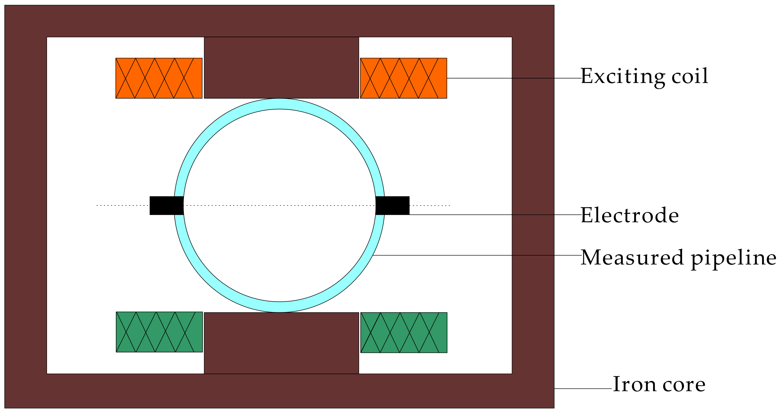
As shown in Figure 1, the detection electrode inside the electromagnetic flowmeter is located on the inner wall of the pipeline and is in contact with the fluid. When the liquid flows through the electrodes, the induced electromotive force will generate a voltage signal between the electrodes. By measuring the magnitude of the voltage signal, the velocity of the fluid can be calculated to realize the flow measurement.
In this paper, stainless steel material is used as the preparation material of the sensor electrode. Stainless steel is widely used in the field of electrode preparation, and its scope of application covers a variety of fluid and environmental conditions. Stainless steel has excellent corrosion resistance to many chemicals, so it is very suitable for liquid flow measurement tasks. In addition, the stainless electrode has outstanding mechanical strength, which is enough to withstand certain stress and pressure, enhancing its reliability under various working conditions.
The structural diagram of the sensor designed in this paper is shown in Figure 1. It consists of a magnetic circuit system composed of an iron core and an excitation coil. When the excitation current is applied, a uniform magnetic field will be generated, thus ensuring that the corresponding induced electromotive force can be obtained on the electrode.
2.3. Design of Hardware Circuit
The hardware circuit of the electromagnetic flowmeter is the supporting platform for the realization of the functions of the whole system. The system design uses SEM32F407ZET6 MCU as the core controller, and all functions of the instrument are realized by the MCU and its peripheral circuits. The MCU controls the ZXMH3A01N8 to generate the excitation signal, which is applied to the excitation coil of the sensor to produce a stable and alternating magnetic field. The analog signal generated by the sensor undergoes amplification and is then routed to the high-precision A/D converter AD7193. The digital signal obtained after A/D conversion is processed by the MCU to calculate instantaneous flow velocity, flow rate, and cumulative flow, which are subsequently displayed in real time on an LCD screen. Parameter configuration can be achieved through keyboard input. Furthermore, the system is equipped with the capability to retain parameters and computed data after power loss.
Figure 2 shows the overall hardware module diagram of the system. The hardware circuit of the system mainly includes a signal conditioning module, power supply and low voltage detection module, A/D sampling module, keyboard and display module, excitation circuit module, and data storage module.
The functions of each module are as follows:
(a) Signal conditioning module: the weak voltage signal output by the electromagnetic flow sensor is amplified, the interference signal unrelated to the measured signal is filtered out, and the useful signal is extracted to provide the amplified voltage analog quantity for the A/D converter.
(b) Power supply and low voltage monitoring module: real-time monitoring of the power supply voltage of the system. When the system voltage is lower than the specified low limit voltage value, the power monitoring module sends an interrupt request to implement power-down protection. That is, before the voltage drops to the working voltage, the important parameters of the system are saved in the memory chip.
(c) A/D sampling module: convert the analog voltage signal processed by the signal amplification processing module into a digital signal and send it to the MCU for processing.
(d) Keyboard and display module: users can set the operating parameters of the instrument using a keyboard, and can also view information such as instantaneous flow rate and velocity of flow on the LCD screen.
(e) Excitation circuit module: it receives the excitation signal from the MCU, amplifies the excitation signal for power, and provides an exciting current to the exciting coil.
(f) Data storage module: stores the configuration parameters and cumulative flow values during the normal operation of the system.
(g) Pulse output module: the pulse output module can output frequency or pulse. The pulse output mode is mainly used for metrological verification. Each pulse output by the MCU represents an equivalent volume of fluid flowing through the measurement pipeline. The frequency output mode is mainly used for control applications, and the output frequency corresponds to the percentage of flow.
(h) Electromagnetic flow sensor: it converts the velocity of the flow signal of the measured fluid into the corresponding electrical signal according to a certain linear function relationship.
2.3.1. Design of Exciting Circuit
The excitation circuit of the electromagnetic flowmeter is the most important part of the system, which is related to the conversion accuracy of the sensor, and also the largest part of the system’s power consumption. Using reasonable excitation technology can not only reduce the power consumption of the system but also improve the measurement accuracy of the system.
In this paper, the electromagnetic flowmeter uses the three-level low-frequency rectangular wave excitation mode to generate the excitation signal . As shown in Figure 3, the excitation is carried out in the intermittent sleep mode with the three values of , 0, and . The sampling period of the electromagnetic flowmeter designed in this paper is , which can be adjusted within 1 s and 15 s according to the different requirements of measurement accuracy and power consumption. When low power consumption is needed, can be set to a larger value, and the measurement accuracy is slightly lower than that of a small , but it meets the accuracy requirements of the electromagnetic flowmeter.
The sampling period is divided into two stages: the excitation stage and dormant stage. During the dormant stage, all other modules except the low-frequency clock of the MCU are closed to reduce the quiescent current and reduce the power consumption of the system. During the excitation stage, the excitation period is set to 160 ms, and the frequency is 6.25 Hz, which is 1/6 of the industrial frequency, which can effectively eliminate the zero-point noise of the flow signal and improve the stability of the zero point of the instrument.
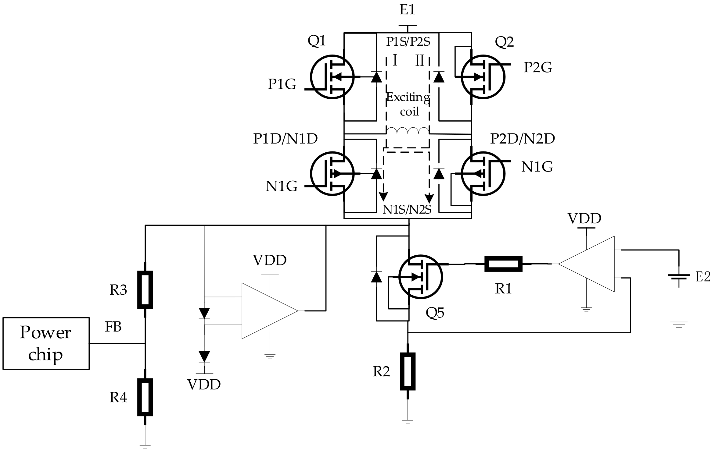
The excitation module determines the magnetic field of the sensor, which is a very important part, related to the stability and transformation accuracy of the magnetic field. The excitation module is essentially an H-bridge circuit driven by a constant current source. In order to reduce the size of the microchip, reduce the power consumption of the system, and improve reliability, this paper uses the integrated bridge chip ZXMHC3A01N8 to design the excitation circuit of the electromagnetic flowmeter, avoiding the use of discrete components to design the excitation circuit, reducing the cost, and improving the reliability of the system.
ZXMHC3A01N8 contains two pairs of complementary N-channel MOSFET and P-channel MOSFET. The high and low levels of the signals loaded on P1G-N2G or P2G-N2G control the on and off of the field-effect transistors, thereby generating an alternating magnetic field in the excitation coil. As shown in Figure 4, the operational amplifier, field-effect transistor Q5, and resistor constitute the constant current source circuit of the system. When P1G-N2G is on, P2G-N1G is off, and the excitation current flows from the power supply E1 in the direction I through the excitation coil, field-effect transistor, and resistor . When P2G-N1G is on, P1G-N2G is off at this time, and the excitation current flows from the power supply in the II direction through the excitation coil, field-effect transistor Q5, and resistor . The magnitude of the current flowing through the excitation coil is determined by the voltage of power supply and resistance (). Since the excitation frequency of this design is controlled by the MCU, it has good adjustability. According to the different fluids being measured, different excitation frequencies can be selected for users to flexibly change.
The authors of this paper selected LMR51420 as the driving power supply of the H-bridge. The circuit is shown in Figure 5. The pin in the figure is connected to a 15 V power supply. The output voltage is connected to the driving pin of ZXMHC3A01N8 to provide the driving current for it. The enable terminal EN is also connected to the 15 V power supply to keep the LMR51420 working.
2.3.2. Design of Core Controller Circuit
In this paper, the electromagnetic flowmeter uses STM32F407ZET6 as the core controller. The STM32F407ZET6 is a powerful microcontroller with high performance, rich peripherals, and flexibility, suitable for a variety of embedded systems and applications, including instrumentation, industrial control, automation, communications, and embedded computing. Multiple low-power consumption modes, ultra-high main frequency, powerful computing power, and rich hardware resources are the main reasons for choosing this model of MCU for this design.
In order to improve accuracy, a 25 MHz external clock is used. In order to filter out the impact of external interference noise and interference noise introduced by the power supply on the microcontroller, a decoupling capacitor is designed between the power supply and the ground of the microcontroller. On the one hand, it functions as an energy storage capacitor to provide and absorb the opening and closing moments of the integrated circuit. The charging and discharging energy, on the other hand, is to filter out the high-frequency noise of the device.
2.3.3. Design of Signal Processing and Sampling Circuit
The signal processing sampling circuit is the hub between the electromagnetic flow sensor and the MCU. Its function is to amplify and filter the induced electromotive force generated by the electromagnetic flow sensor, and then send it to the ADC for conversion. The converted digital signal is sent to the MCU for further processing. The flow chart of signal processing and sampling is shown in Figure 6.
The electromagnetic flow sensor outputs a weak alternating signal (microvolt level), and the internal impedance of the signal is high. The amplitude of the noise signal is much larger than the measured signal, so the signal generated by the sensor needs to be amplified, and the magnification is controllable by the MCU. An integrating circuit is designed to compensate for the DC offset feedback in the signal. In order to filter out noise and interference signals, it is necessary to design a high-quality filter circuit to filter out noise and interference signals in order to meet the accuracy requirements of the instrument.
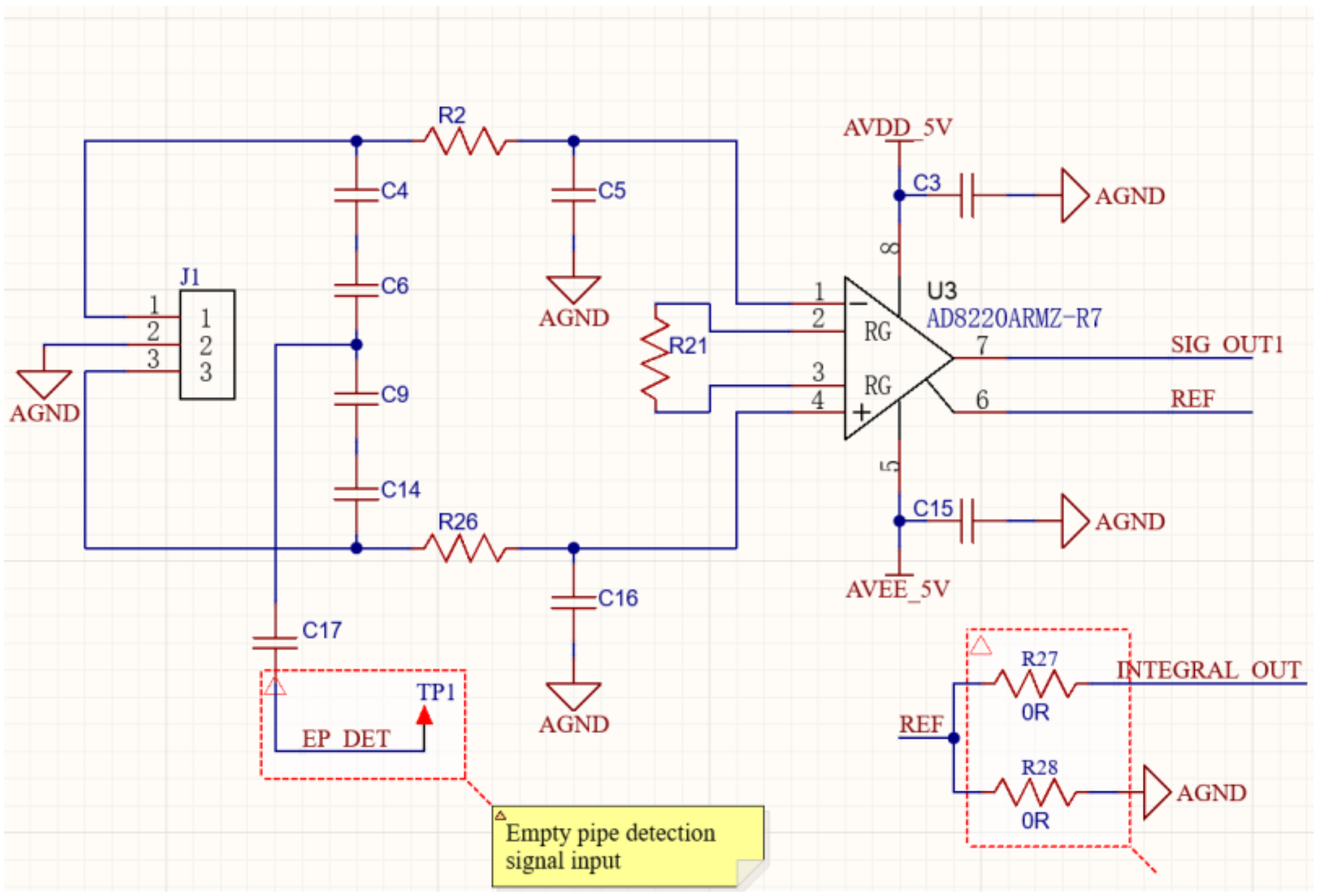
As shown in Figure 7, the induced electromotive force output by the electromagnetic flow sensor first passes through a filtering circuit composed of an RC to filter out the noise interference signals. Then, a high common-mode rejection ratio amplification circuit composed of an adjustable gain and differential input AD8220 instrument amplifier is used to amplify the signal, thereby suppressing the interference signal.
As shown in Figure 8, a high-performance and low-power TL071H operational amplifier is used to form an integral feedback circuit, which can provide DC offset feedback compensation for the above output signal.
The flow signal output by the electromagnetic flow sensor is amplified by the instrument amplifier, and must be filtered, amplified, and rectified to effectively improve the SNR of the flow signal, laying the foundation for establishing the relationship between the flow signal and the flow rate. As shown in Figure 9, a low-noise TL072 operational amplifier and RC low-pass filter are used to form an amplification and filtering circuit to amplify and filter the above signal.
Since there is a linear relationship between the flow rate and the voltage signal output by the sensor, the signals corresponding to different flow rates require different amplification factors. For this purpose, the signal needs to go through an adjustable gain amplification circuit after being amplified and filtered by the previous stage. As shown in Figure 10, a low-noise TL072 operational amplifier and resistors with different resistance values are used to form a six-level adjustable gain circuit. The gain of the amplifier circuit is changed according to the amplitude of the input signal, and the gain is adjustable through the MCU.
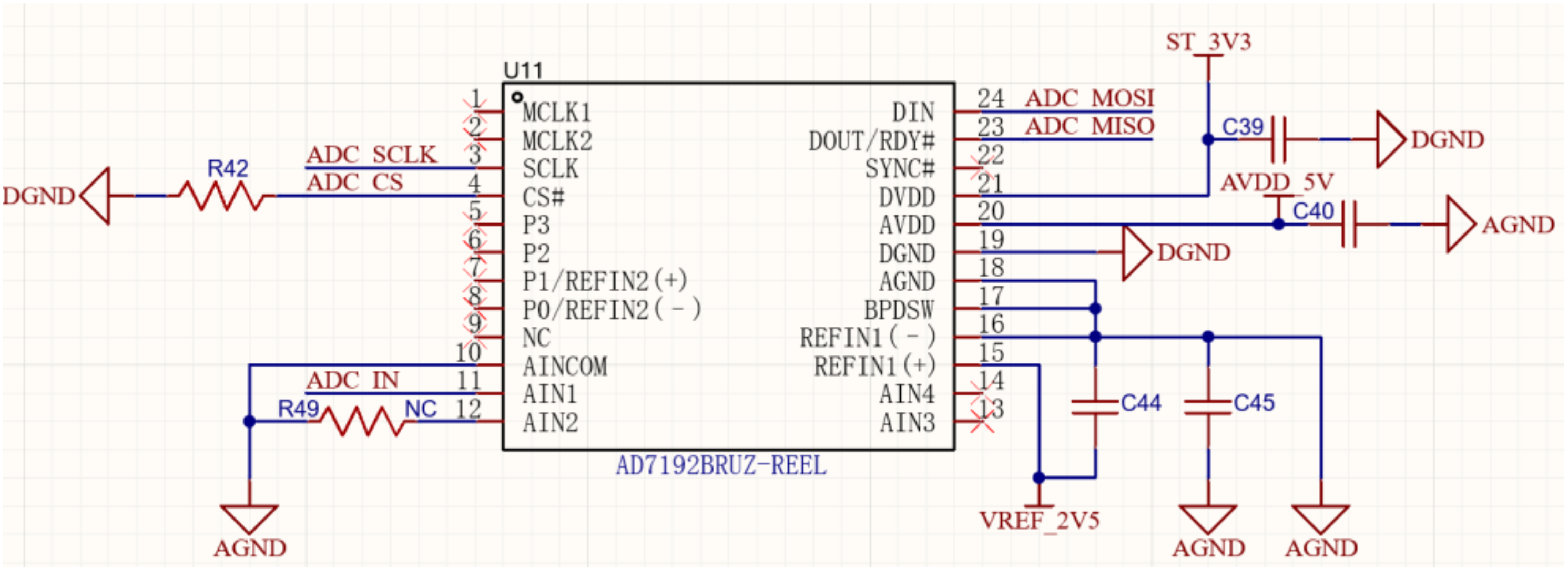
The signal output by the sensor is amplified and filtered before being sent to the A/D converter. As shown in Figure 11, this design adopts a high-precision analog-to-digital converter AD7912 with a resolution of up to 24 bits, which is suitable for high-precision measurement and has low noise.
2.3.4. Design of Empty Pipe Detection Circuit
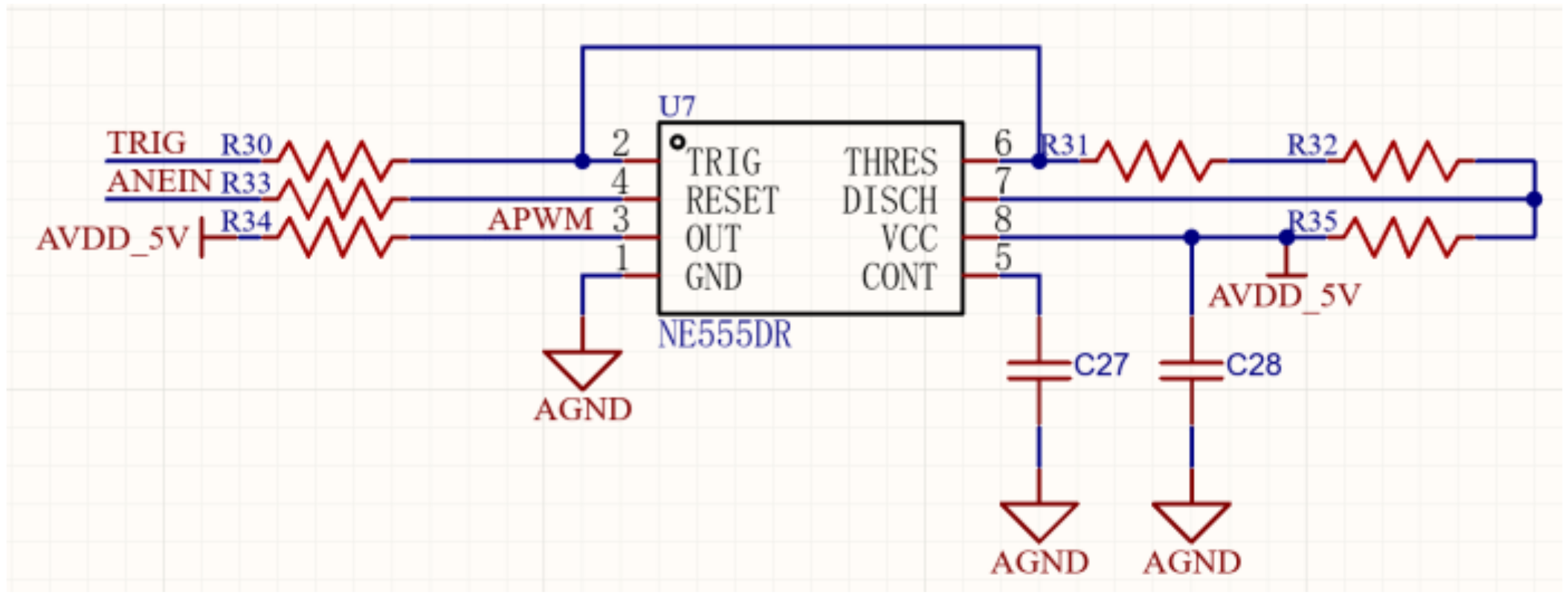
When using an electromagnetic flowmeter, it is necessary to ensure that the measuring pipeline of the electromagnetic flowmeter is filled with the measured liquid. This is because when the measuring pipeline is not full, the data detected by the sensor cannot accurately reflect the flow rate of the measured fluid. If the electrodes inside the measuring pipe are completely exposed to the air, the sensor will generate a significant interference signal, causing significant oscillation in the output signal, seriously affecting the normal use of the electromagnetic flowmeter. In practical measurement, it is difficult to ensure that the pipeline is always filled with liquid, so real-time detection of empty pipe status and providing warnings are crucial for the signal processing of electromagnetic flowmeters. The empty pipe detection circuit designed for this system is shown in Figure 12, which uses the NE555 timer chip and is configured as a monostable mode. When the liquid level in the pipeline falls below or exceeds the threshold, the input state of the circuit will change, triggering the monostable state of the NE555 timer. The NE555 starts charging the capacitor until it reaches the threshold voltage. Once the capacitor is charged to the threshold voltage, the output state of NE555 will change and trigger the connection operation. When the tested pipeline is not empty, the timer cannot be triggered to work, and the timer output is at a low level. When the measured pipeline is an empty pipeline, the input signal pulse of the sensor continuously triggers the timer, and the output signal of the timer is always at a high level. Therefore, as long as the MCU detects the output signal of the timer, it can determine whether it is an empty pipe.
2.4. Design of System Software
The system software is written using a modular design method, consisting of a main program, interrupt program, excitation signal generation, A/D sampling, communication, display, and keyboard service subroutines. As shown in Figure 13, after the system is powered on, various modules of the system are initialized, including completing the configuration of I/O ports and registers, initializing clocks and peripheral circuits, and loading data from EEPROM to complete the configuration of system operating parameters. After the system initialization is completed, set the open interrupt program and wait for timed interrupt processing. By responding to each sub-module, determine whether each module is running normally. The MCU reads the A/D sampling value, calculates the flow rate for one excitation cycle, and then corrects the flow rate value, and sequentially performs median filtering and mean filtering on it. Finally, it is demanded to calculate the instantaneous flow rate and send it to the LCD for real-time display.
3. Simulation and Measured Results of Electromagnetic Flowmeter
This chapter will analyze the simulation and test results of the main modules of the system hardware circuit, and then analyze the overall test results of the system, and establish a relationship with the flow based on the final output flow signal of the system.
3.1. Simulation and Measured Results of Hardware Circuit
The debugging of hardware circuits can mainly be divided into simulation, measuring, and analysis of signal processing circuits.
3.1.1. Simulation of Signal Processing Circuit
As shown in Figure 14, a low-frequency rectangular wave of 170 V, 6.25 Hz, and a duty ratio of 50% was used in the simulation process to replace the input signal of the signal processing circuit, which is of the same frequency as the flow signal.
After observing with an oscilloscope, the signal waveform output by the integral feedback circuit during the simulation process is shown in Figure 15. However, the waveform of the signal still has rectangular wave characteristics, playing a role in the DC offset and feedback compensation for the flow signal.
The flow signal undergoes a series of processing, such as amplification and filtering, and the final output signal waveform is shown in Figure 16. From the figure, it can be seen that there are spikes in the output waveform at the point of the signal polarity alternation, which is mainly caused by the insufficient switching speed of the switching diode and the phase delay introduced by the integrator and the presence of nonlinear components. However, the signal still has the characteristic of a rectangular wave, which does not affect ADC sampling.
3.1.2. Measurement of Signal Processing Circuit
The experiment measures the voltage amplitude of the flow signal output by the signal processing circuit by taking the average of multiple measurements. From the theoretical values in Section 2, it can be seen that the output voltage of the signal processing circuit should theoretically maintain a linear relationship with the flow rate. Therefore, in the experiment, the proportional coefficient K is used to determine whether the flow rate is linearly related to the output voltage. The expression for the proportional coefficient of the i-th measurement point is the following:
Here represents the average instantaneous flow rate after multiple measurements at the i-th detection point, and represents the average voltage value after multiple measurements at the i-th detection point.
Due to the unknown proportion coefficient K of the true point, a correction factor needs to be added to correct the measured flow rate. The measurement data is shown in Table 1, which records the flow values before and after correction, as well as the corresponding output voltage at that flow rate.
As shown in Figure 17, comparing the theoretical verification values of the flow rate, the corrected flow rate values are consistent with the trend, indicating that the design of the entire system is consistent with the theory. By comparing the flow rate values before correction, it can be found that the corrected flow rate curve is closer to the theoretical flow rate value, indicating that the testing of the system is correct.
As shown in Figure 18, it can be seen that there is a good linear relationship between the voltage value of the output signal and the measured flow rate, which is consistent with the theory in Section 2. Meanwhile, it can be seen that the proportional coefficients remain around 0.0765, indicating that the electromagnetic flowmeter is working normally. When the flow rate is small, the proportion coefficient is relatively large, which may be caused by the small output signal being affected by noise interference at this time.
The signal output by the signal conditioning module at flow rates of 0.2 m/s and 2.0 m/s are measured, as shown in Figure 19a and Figure 19b, respectively. Comparing the two graphs, it can be seen that the noise at 0.2 m/s is significantly higher than that at 2 m/s. According to the measured data, the signal fluctuation at both flow rates is approximately 23 mV. However, when the flow rate is low, the proportion of noise is high, and when the flow rate is high, the proportion of noise is low. Therefore, when the flow rate is low, the interference from noise is greater.
3.2. Measurement of Overall System
The proposed electromagnetic flowmeter was calibrated by comparing it with the standard electromagnetic flowmeter. A standard flowmeter with a higher accuracy is used to connect with the proposed flowmeter in series, allowing fluid to flow through both at the same time. By comparing the indications of the flowmeters, the error of the proposed meter is determined to achieve the purpose of calibration. Here, the flow rate value of the proposed electromagnetic flowmeter is compared with the flow rate value measured by the standard meter under different flow rates to determine the relative indication error of the electromagnetic flowmeter.
The relative error calculation method for the flow rate of electromagnetic flowmeters is as follows:
Here represents the relative indication error of the measured flowmeter during a certain detection at the detection point, represents the flow rate displayed by the proposed flowmeter during a certain detection at the detection point, in , and represents the flow rate displayed by the standard flowmeter during a certain detection at the detection point, in .
The average error of each calibration point of the electromagnetic flowmeter is:
Here represents the average relative error of the measured point, represents the number of measurements at the detection point, and represents the relative indication error of the i-th measurement at the measured point.
The repeatability of electromagnetic flowmeters refers to the degree to which the measurement results of the same measured quantity are consistent among different observers under different measurement conditions and in different measurement environments. It is an important performance indicator of electromagnetic flowmeters. If each measured point is measured n times, the repeatability calculation formula for that flow point is [14]:
Here represents the repeatability of the measured point. This experiment set up six measured points and used the above formula to calculate the error and repeatability of the measured data. The measured results are shown in Table 2.
From Table 2, it can be seen that the relative indication error of the electromagnetic flowmeter designed in this article is within 0.3%, and the repeatability fluctuates within the range of 0.03%, which is less than 1/10 of the maximum allowable error. Therefore, the accuracy of the flowmeter meets the design accuracy requirements.
4. Conclusions
This paper designs an intelligent electromagnetic flowmeter for coal mines. Firstly, the working principle of the electromagnetic flowmeter was analyzed, providing a theoretical basis for the design of the electromagnetic flowmeter. Subsequently, the electromagnetic flow sensor, excitation circuit, core control circuit, signal conditioning circuit, and empty pipe detection circuit were analyzed and designed in sequence. High-performance and low-power MCU and high-precision chips were selected to ensure measurement accuracy and reduce power consumption. In the software design section, a low-frequency rectangular wave excitation method is used to extend the battery life. Finally, the performance of the electromagnetic flowmeter was measured, and the measured data showed that the measured flow rate was basically linear with the output voltage. The relative indication error of the electromagnetic flowmeter was within 0.3%, and the repeatability fluctuated within the range of 0.03%. Therefore, the flowmeter has good measurement accuracy and is suitable for long-term use in coal mining environments.
Author Contributions
Methodology, N.L.; writing—original draft preparation, B.C.; writing—review and editing, M.T., Q.Y., B.J. and J.L. All authors have read and agreed to the published version of the manuscript.
Funding
This research received no external funding.
Data Availability Statement
These data are unavailable due to privacy or ethical restrictions in this paper.
Conflicts of Interest
B.C., M.T. and J.L. was employed by the company Shaanxi Taihe Intelligent Drilling Co., Ltd. The remaining authors declare that the research was conducted in the absence of any commercial or financial relationships that could be construed as a potential conflict of interest.
References
- Wang, L.; Deng, J.; Han, H. Design of electromagnetic flow converters. Autom. Instrum. 2022, 204–209. [Google Scholar]
- Fox, C.; Morrison, M.E.K. On the spatial response of electromagnetic flowmeters. Appl. Sci. 2023, 13, 6531. [Google Scholar] [CrossRef]
- Michalski, A.; Starzynski, J.; Wincenciak, S. Optimal design of the coils of an electromagnetic flow meter. IEEE Trans. Magn. 1998, 34, 2563–2566. [Google Scholar] [CrossRef]
- Li, B.; Liu, J.; Chen, J. Signal Processing Method of Harmonic Analysis Slurry Electromagnetic Flowmeter Based on Walsh Transform. In Proceedings of the 2020 International Conference on Artificial Intelligence and Electromechanical Automation (AIEA), Tianjin, China, 26–28 June 2020; pp. 542–546. [Google Scholar]
- Li, B.; Yan, Y.; Chen, J. Signal Processing Scheme of Step Excitation Electromagnetic Flowmeter Based on Outlier Elimination and Double Median Filtering. In Proceedings of the 2020 6th International Conference on Control, Automation and Robotics (ICCAR), Singapore, 20–23 April 2020; pp. 632–637. [Google Scholar]
- Xu, X.; Liu, K.; Qin, Y. The Excitation System of Low-Frequency Rectangular Wave in Electromagnetic Flowmeter Based on Finite Element Analysis. In Proceedings of the 2011 IEEE 3rd International Conference on Communication Software and Networks, Xi’an, China, 27–29 May 2011; pp. 711–714. [Google Scholar]
- Huang, X.; Yue, S. The energy-saving strategy of electromagnetic flowmeters based on various predicting methods. IEEE Trans. Appl. Supercond. 2016, 26, 1–5. [Google Scholar] [CrossRef]
- Michalski, A. A new approach to estimating the main error of a primary transducer for an electromagnetic flowmeter. IEEE Trans. Instrum. Meas. 2001, 50, 764–767. [Google Scholar] [CrossRef]
- Michalski, A. Dry calibration procedure of electromagnetic flowmeter for open channels. IEEE Trans. Instrum. Meas. 2000, 49, 434–438. [Google Scholar] [CrossRef]
- Maalouf, A.I. The derivation and validation of the practical operating equation for electromagnetic flowmeters: Case of having an electrolytic conductor flowing through. IEEE Sens. J. 2006, 6, 89–96. [Google Scholar] [CrossRef]
- Polo, J.; Pallas-Areny, R.; Mardn-Vide, J.P. Analog signal processing in an AC electromagnetic flowmeter. IEEE Trans. Instrum. Meas. 2002, 51, 793–797. [Google Scholar] [CrossRef]
- Michalski, A.; Starzynski, J.; Wincenciak, S. 3-D approach to designing the excitation coil of an electromagnetic flowmeter. IEEE Trans. Instrum. Meas. 2002, 51, 833–839. [Google Scholar] [CrossRef]
- Mitchell, B.; Zhou, Y.; Hayes, M.P.; Heffernan, B.; Platt, L.; Bailey, J.; Hunze, A.; Gao, K.; Long, N.; Woodhead, L. Non-Invasive groundwater velocity measurements using a novel electromagnetic flowmeter. IEEE Trans. Instrum. Meas. 2022, 71, 1–15. [Google Scholar] [CrossRef]
- Linnert, M.A.; Mariager, S.O.; Rupitsch, S.J.; Lerch, R. Dynamic offset correction of electromagnetic flowmeters. IEEE Trans. Instrum. Meas. 2019, 68, 1284–1293. [Google Scholar] [CrossRef]
- Jin, N.; Yu, C.; Han, Y.; Yang, Q.; Ren, Y.; Zhai, L. The performance characteristics of electromagnetic flowmeter in vertical low-velocity oil-water two-phase flow. IEEE Sens. J. 2021, 21, 464–475. [Google Scholar] [CrossRef]
- Michalski, A.; Jakubowski, J. An energy-saving algorithm for electromagnetic flow measurement in open channels [Instrumentationnotes]. IEEE Instrum. Meas. Mag. 2011, 14, 40–45. [Google Scholar] [CrossRef]
- Michalski, A.; Jakubowski, J.; Watral, Z. The problems of pulse excitation in electromagnetic flowmeters [Instrumentationnotes]. IEEE Instrum. Meas. Mag. 2013, 16, 47–52. [Google Scholar] [CrossRef]
- Maalouf, A.I. A validated model for the zero drift due to transformer signals in electromagnetic flowmeters operating with electrolytic conductors. IEEE Sens. J. 2006, 6, 1502–1510. [Google Scholar] [CrossRef]
- Ge, L.; Chen, J.; Tian, G.; Zeng, W.; Huang, Q.; Hu, Z. Study on a new electromagnetic flow measurement technology based on differential correlation detection. Sensors 2020, 20, 2489. [Google Scholar] [CrossRef] [PubMed]
- Wang, Y.; Li, H.; Liu, X.; Zhang, Y.; Xie, R.; Huang, C.; Hu, J.; Deng, G. Novel downhole electromagnetic flowmeter for oil-water two-phase flow in high-water-cut oil-producing wells. Sensors 2016, 16, 1703. [Google Scholar] [CrossRef] [PubMed]
Figure 1.
Sensor structure of electromagnetic flowmeter.

Figure 2.
Overall hardware circuit architecture of the system.

Figure 3.
Three-level low-frequency rectangular wave excitation.

Figure 4.
Schematic diagram of constant current exciting circuit.

Figure 5.
LMR51420 peripheral circuit.

Figure 6.
Signal processing and sampling process.

Figure 7.
High-impedance instrument amplification circuit.

Figure 8.
Integral feedback circuit.

Figure 9.
Filter and amplification circuit.

Figure 10.
Adjustable gain amplification circuit.

Figure 11.
A/D sampling circuit.

Figure 12.
Empty pipe detection circuit.

Figure 13.
Flow chart of system software design.

Figure 14.
Input signal of signal processing circuit.

Figure 15.
Output signal of the integral feedback circuit.

Figure 16.
Output signal of the signal processing circuit.

Figure 17.
Measured flow data curve.

Figure 18.
The relationship curve between the flow rate at the measurement point and the proportional coefficient K.
Figure 18.
The relationship curve between the flow rate at the measurement point and the proportional coefficient K.

Figure 19.
Output signals by the signal conditioning module under different flow velocities. (a) 0.2 m/s. (b) 2 m/s.
Figure 19.
Output signals by the signal conditioning module under different flow velocities. (a) 0.2 m/s. (b) 2 m/s.


Table 1.
Measured data for flow rate and output voltage.
| Theoretical Verification Value of Flow Rate ) | Flow Rate before Correction ) | Flow Rate after Correction ) | Output Voltage (mV) |
|---|---|---|---|
| 1.64 | 1.641 | 1.643 | 20.975 |
| 2.6 | 2.601 | 2.598 | 33.821 |
| 3.110 | 3.110 | 40.452 | |
| 7.802 | 7.779 | 102.607 | |
| 15.5 | 14.787 | 15.024 | 196.680 |
| 20.5 | 20.004 | 20.104 | 265.412 |
| 25 | 24.273 | 24.564 | 321.652 |
Table 2.
Measured data for flow rate.
| Calibration Flow Rate Point ) | Standard Meter Flow Rate ) | The Proposed Meter Flow Rate ) | Relative Indication Error (%) | Mean Error (%) | Repeatability (%) |
|---|---|---|---|---|---|
| 2.3 | 2.332 | 2.336 | 0.17 | 0.19 | 0.019 |
| 2.332 | 2.337 | 0.21 | |||
| 2.330 | 2.341 | 0.47 | |||
| 2.331 | 2.329 | 0.09 | |||
| 2.332 | 2.333 | 0.04 | |||
| 2.333 | 2.337 | 0.17 | |||
| 2.8 | 2.809 | 2.803 | 0.21 | 0.21 | 0.006 |
| 2.804 | 2.811 | 0.25 | |||
| 2.805 | 2.810 | 0.18 | |||
| 2.808 | 2.813 | 0.18 | |||
| 2.805 | 2.815 | 0.36 | |||
| 2.808 | 2.811 | 0.11 | |||
| 2.807 | 2.812 | 0.18 | |||
| 4.31 | 4.317 | 4.327 | 0.23 | 0.19 | 0.009 |
| 4.322 | 4.310 | 0.28 | |||
| 4.326 | 4.318 | 0.18 | |||
| 4.324 | 4.324 | 0.00 | |||
| 4.328 | 4.319 | 0.21 | |||
| 4.322 | 4.310 | 0.28 | |||
| 4.326 | 4.318 | 0.18 | |||
| 8.92 | 8.925 | 8.904 | 0.24 | 0.22 | 0.005 |
| 8.924 | 8.901 | 0.26 | |||
| 8.912 | 8.898 | 0.16 | |||
| 8.916 | 8.908 | 0.09 | |||
| 8.918 | 8.893 | 0.28 | |||
| 8.926 | 8.904 | 0.25 | |||
| 8.928 | 8.905 | 0.26 | |||
| 13.54 | 13.530 | 13.523 | 0.05 | 0.16 | 0.015 |
| 13.543 | 13.534 | 0.07 | |||
| 13.551 | 13.514 | 0.27 | |||
| 13.525 | 13.475 | 0.37 | |||
| 13.533 | 13.507 | 0.19 | |||
| 13.541 | 13.527 | 0.10 | |||
| 13.523 | 13.512 | 0.08 | |||
| 17.91 | 17.911 | 17.916 | 0.03 | 0.24 | 0.028 |
| 17.922 | 17.852 | 0.39 | |||
| 17.910 | 17.847 | 0.35 | |||
| 17.925 | 17.923 | 0.01 | |||
| 17.905 | 17.938 | 0.18 | |||
| 17.928 | 17.858 | 0.39 | |||
| 17.935 | 17.876 | 0.33 |
Disclaimer/Publisher’s Note: The statements, opinions and data contained in all publications are solely those of the individual author(s) and contributor(s) and not of MDPI and/or the editor(s). MDPI and/or the editor(s) disclaim responsibility for any injury to people or property resulting from any ideas, methods, instructions or products referred to in the content. |
© 2024 by the authors. Licensee MDPI, Basel, Switzerland. This article is an open access article distributed under the terms and conditions of the Creative Commons Attribution (CC BY) license (https://creativecommons.org/licenses/by/4.0/).
Share and Cite
MDPI and ACS Style
Cheng, B.; Tong, M.; Yan, Q.; Jin, B.; Liu, N.; Lu, J. Portable Intelligent Electromagnetic Flowmeter Controlled by Magnetic Induction Intensity. Electronics 2024, 13, 556. https://0-doi-org.brum.beds.ac.uk/10.3390/electronics13030556
AMA Style
Cheng B, Tong M, Yan Q, Jin B, Liu N, Lu J. Portable Intelligent Electromagnetic Flowmeter Controlled by Magnetic Induction Intensity. Electronics. 2024; 13(3):556. https://0-doi-org.brum.beds.ac.uk/10.3390/electronics13030556
Chicago/Turabian StyleCheng, Binbin, Minbo Tong, Qilong Yan, Bochuan Jin, Nengwu Liu, and Jiarui Lu. 2024. "Portable Intelligent Electromagnetic Flowmeter Controlled by Magnetic Induction Intensity" Electronics 13, no. 3: 556. https://0-doi-org.brum.beds.ac.uk/10.3390/electronics13030556
Note that from the first issue of 2016, this journal uses article numbers instead of page numbers. See further details here.