Pruning Deep Neural Network Models via Minimax Concave Penalty Regression

School of Science, Hubei University of Technology, Wuhan 430068, China
*
Author to whom correspondence should be addressed.
Appl. Sci. 2024, 14(9), 3669; https://0-doi-org.brum.beds.ac.uk/10.3390/app14093669
Submission received: 1 March 2024
/
Revised: 22 April 2024
/
Accepted: 23 April 2024
/
Published: 25 April 2024
Abstract
:In this study, we propose a filter pruning method based on MCP (Minimax Concave Penalty) regression. The convolutional process is conceptualized as a linear regression procedure, and the regression coefficients serve as indicators to assess the redundancy of channels. In the realm of feature selection, the efficacy of sparse penalized regression gradually outperforms that of Lasso regression. Building upon this insight, MCP regression is introduced to screen convolutional channels, coupled with the coordinate descent method, to effectuate model compression. In single-layer pruning and global pruning analyses, the Top1 loss value associated with the MCP regression compression method is consistently smaller than that of the Lasso regression compression method across diverse models. Specifically, when the global pruning ratio is set to 0.3, the Top1 accuracy of the MCP regression compression method, in comparison with that of the Lasso regression compression method, exhibits improvements of 0.21% and 1.67% under the VGG19_Simple and VGG19 models, respectively. Similarly, for ResNet34, at two distinct pruning ratios, the Top1 accuracy demonstrates enhancements of 0.33% and 0.26%. Lastly, we compare and discuss the novel methods introduced in this study, considering both time and space resource consumption.
1. Introduction
Deep learning stands as a pivotal research focus within the realm of machine learning, playing a crucial role in domains such as data mining and natural language processing. At the core of deep learning’s evolution are deep neural networks, encompassing diverse network layers designed for the extraction of target feature information and the acceleration of computational processes [1]. Typically, the learning capacity of deep neural networks correlates positively with the depth of network layers, especially at higher computational volumes. However, this advantage comes with accompanying challenges, including elevated storage costs, increased computational demands, and heightened energy consumption. These factors impose limitations on the advancement of deep neural networks, particularly in the context of real-time processing tasks and deployment on mobile devices [2].
Primarily, deep neural networks encounter challenges related to storage space. Initial investigations revealed a positive correlation between the number of model parameters and the likelihood of convergence, leading to enhanced accuracy. For instance, the early LeNet-5 comprised approximately 430K parameters [3], while the subsequent VGG-16 model boasted a significantly larger parameter count of 138 M [4]. The substantial expansion of storage capacity in mobile devices poses a hindrance to the advancement of neural network technology. Additionally, in terms of computational aspects, deep neural networks present challenges of high computation complexity, coupled with excessive demand for storage space. For instance, during the neural network learning process, rapid convolutional operations on multi-dimensional matrices are imperative, involving a plethora of matrix operations [5]. Furthermore, in the domain of energy consumption, deep neural networks, characterized by multiple layers of interconnected neurons and variables, exhibit considerable storage and power demands across diverse embedded applications. Notably, the initial fully connected level of VGGNet encompasses 100 M, with a maximum mass of 140 M, contributing substantially to heightened energy consumption [6].
Confronted with the burgeoning storage requirements of deep neural networks, the training of extensive networks necessitates a substantial volume of computations and energy consumption. Moreover, given that the training of large networks is predominantly executed on high-performance servers or clusters, the direct application of these procedures to mobile devices becomes impractical. Consequently, research on techniques related to the compression and acceleration of deep neural networks has emerged to address these challenges. Recent studies, including references [7,8,9,10], have also reviewed model compression methods in the last few years.
The complexity of a deep neural network model is determined by its parameters, prompting researchers to prioritize a reduction in network parameters as a primary avenue for compressing and optimizing the model. Geng and Niu [11] proposed a classification of model compression methods, distinguishing between shallow compression and deep compression. Shallow compression encompasses filter-level pruning and knowledge distillation. Regarding the latter, Si and Qi [12] contend that knowledge distillation methods treat the neural network holistically. These methods employ a learning approach to train a smaller network guided by a larger network with comparable performance, indirectly achieving the goal of compression.
Due to the simplicity of the network architecture and the limited significance of the relationship between model performance and size in stochastic neural networks, Hu and Gao [13] proposed a self-distillation pipeline tailored for such networks. Given the complexity of deep neural network models, making predictions that are challenging to comprehend and examine, Liu and Wang [14] employed knowledge distillation techniques to distill deep neural networks into decision trees, pioneering the distillation of deep neural networks into ordinary decision trees for multi-class datasets. In response to the advancements in deep neural networks and knowledge distillation, Zhang et al. [15] introduced a novel form of self-distillation distinct from traditional knowledge distillation. This form involves the transfer of knowledge within the same model, specifically from deep layers to shallow layers. Building on earlier research in knowledge distillation, Ning et al. [16] summarized the challenges associated with this approach, including the complexity of the training process, issues related to model alignment and hyperparameter tuning, and limitations in practical scenarios.
Chang [17] contends that deep convolutional neural network pruning distinguishes itself among various network compression methods due to its flexible operation, pronounced compression and acceleration effects, and minimal performance loss. This approach has garnered significant attention and research. LeCun [18] evidenced this approach, garnering significant attention and research, validating the method’s importance in assessing the impact of parameters on the objective function. The fundamental concept involves utilizing second-order derivatives to strike a balance between network complexity and test errors, a principle referred to as the “Optimal Brain Damage (OBD) method”. Hassibi and Stork [19] evidenced the Optimal Brain Surgeon (OBS) concept, which shares similarities with the Optimal Brain Damage (OBD) method, validating the work’s significance in the field. However, the authors demonstrate that OBS offers greater ease of implementation for smaller networks, with computational challenges escalating as the network size increases. In contemporary research, structured pruning has become a prevalent technique for model compression. In the realm of layer pruning, Wu et al. [20] noted that distinct layers exhibit varying pruning requirements. To address this, they proposed a differentially evolved hierarchical weight pruning method. This method effectively compressed the parameters of LeNet-300-100, LeNet-5, AlexNet, and VGG16, resulting in compression ratios of 24×, 14×, 29×, and 12×, respectively. In contrast, Xu et al. [21] extended the layer pruning method by incorporating sparsity into the training process. They utilized the original convolutional layers to transform them into fusible residual convolutional blocks, thus amalgamating the benefits of short inference time and effective pruning. Addressing filter pruning, Li et al. [22] introduced a channel pruning compression method to enhance filter resilience and reduce the size of the neural network. They proposed a composite channel pruning approach, utilizing improved L1 regularization training and a global filter importance degree. Zhang et al. [23] introduced a pruning algorithm designed to address the issue, wherein the deletion of less important filters often results in an imbalanced filter paradigm distribution. This algorithm not only identifies and retains filters aligned with the original paradigm distribution but also eliminates redundant filters. In a similar vein, Geng and Niu [24] suggested an enhancement in the pruning direction. Specifically, they proposed a backward layer-by-layer filter pruning approach, starting from the last convolutional layer. This strategy proves effective in mitigating accuracy loss by preventing the premature removal of shallow convolutional filters.
Chen and Wang [25] underscore the importance of regularization, employed to mitigate model overfitting and minimize generalization errors. They argue that, with the increasing depth of neural networks, there is a corresponding expansion in model complexity and untrained parameters. Therefore, the judicious use of regularization becomes particularly crucial to forestall model overfitting. Alemu et al. [26] introduced a group Lasso regularization term as an effective hidden layer regularization method for feedforward neural networks, serving as an efficient means to eliminate redundant or unnecessary neurons within the feedforward neural network structure. In a parallel effort, Lin et al. [27] devised both inter-group and intra-group unbiased structured sparse regularizers. These sparsity constraints were selectively applied to address redundant neurons and the redundant weights of the remaining neurons. Simultaneously, they formulated an unbiased sparse regularized compression model, featuring a dual-strategy structure for neural networks with dual-strategy regularization.
The introduction of regularization penalties applied to variables has led to the application of various penalties in the field of variable selection. Ridge regression utilizes L2 regularization penalties to mitigate the impact of covariance between variables by identifying redundant variables through Ridge traces. Tibshurani’s proposed Lasso (Least Absolute Shrinkage and Selection Operation) regression, incorporating L1 regularization penalties, automatically selects variables during regression coefficient estimation and compresses the coefficients of redundant variables to zero. He [28] pioneered the application of Lasso regression in model compression, successfully eliminating redundant channels. Wang and Sun [29] employed the Lasso method to identify key factors influencing house prices in China’s provinces. They identified a significant error in this method and proposed mitigating the bias in Lasso estimation by incorporating SCAD and MCP (Minimax Concave Penalty). Farbahri et al. [30] investigated three regression methods on variables with the greatest impact on fasting blood glucose, including the use of Lasso regression to select variables, such as HbA1c, urea, age, BMI, genetics, and gender. Wu et al. [31] relied on Lasso regression for channel selection, and they fused Lasso regression with Singular-Value Decomposition (SVD) to expedite parameter compression.
In the context of channel selection, Lasso employs a constant penalty strength for regression coefficients, whereas MCP applies differentiated penalties. MCP adheres to the principle of imposing greater penalties on coefficients closer to zero and smaller penalties on larger coefficients, enhancing the identification of redundant features. Lee and Kim [32] contend that penalized regression optimization is more straightforward and cost-effective compared with subset selection. Moreover, as the number of features increases, penalized regression can be effectively controlled by one or a few tuning parameters, whereas subset selection is hindered by combinatorial explosions in computation. Xu and Lei [33] introduce sparsity to original variables and augment sparse regression into traditional principal component analysis, retaining the merits of traditional principal component analysis while improving model estimation accuracy due to sparsity. Lin et al. [34] propose a variable selection method for functional regression models applied to sparse functional-type data. They performed functional principal component analysis on sparse functional-type independent variables based on conditional expectation, using the estimated orthogonal eigenfunctions as basis functions for model expansion. Yoshida [35] incorporates linear quantiles for high-dimensional data in regression and variable selection. To achieve variable selection, a group Lasso-type sparse penalty is employed to estimate the nonzero coefficient function at the quantile level. Shin et al. [36] advocate using Lasso and group Lasso penalty functions simultaneously at the node and predictor variable levels in a sparse neural network regression method based on a single hidden layer architecture and sparse induced penalties. Additionally, statistical studies [37,38,39] demonstrate that sparse penalized regression outperforms Lasso regression in feature selection. Building on this, MCP regression is introduced into the model compression process to customize the network model by filtering the output feature map channels.
2. Methodological Models
2.1. Common Layers in Convolutional Neural Networks
2.1.1. Fully Connected Layer
The fully connected layer consists of multiple neurons interconnected according to specific rules. Figure 1 illustrates the computational flow of a single neuron on the left and the network constituted by the fully connected layer on the right.
The leftmost layer is called the input layer, responsible for receiving input data; the rightmost layer is called the output layer, from which the neural network’s output data can be obtained. The layers between the input and output layers are called hidden layers. There are no connections between neurons in the same layer. Each neuron in the Nth layer is connected to all neurons in the (N-1)th layer, where the output of the neurons in the (N-1)th layer serves as the input for the neurons in the Nth layer. Each connection has a weight.
2.1.2. Convolutional Layer
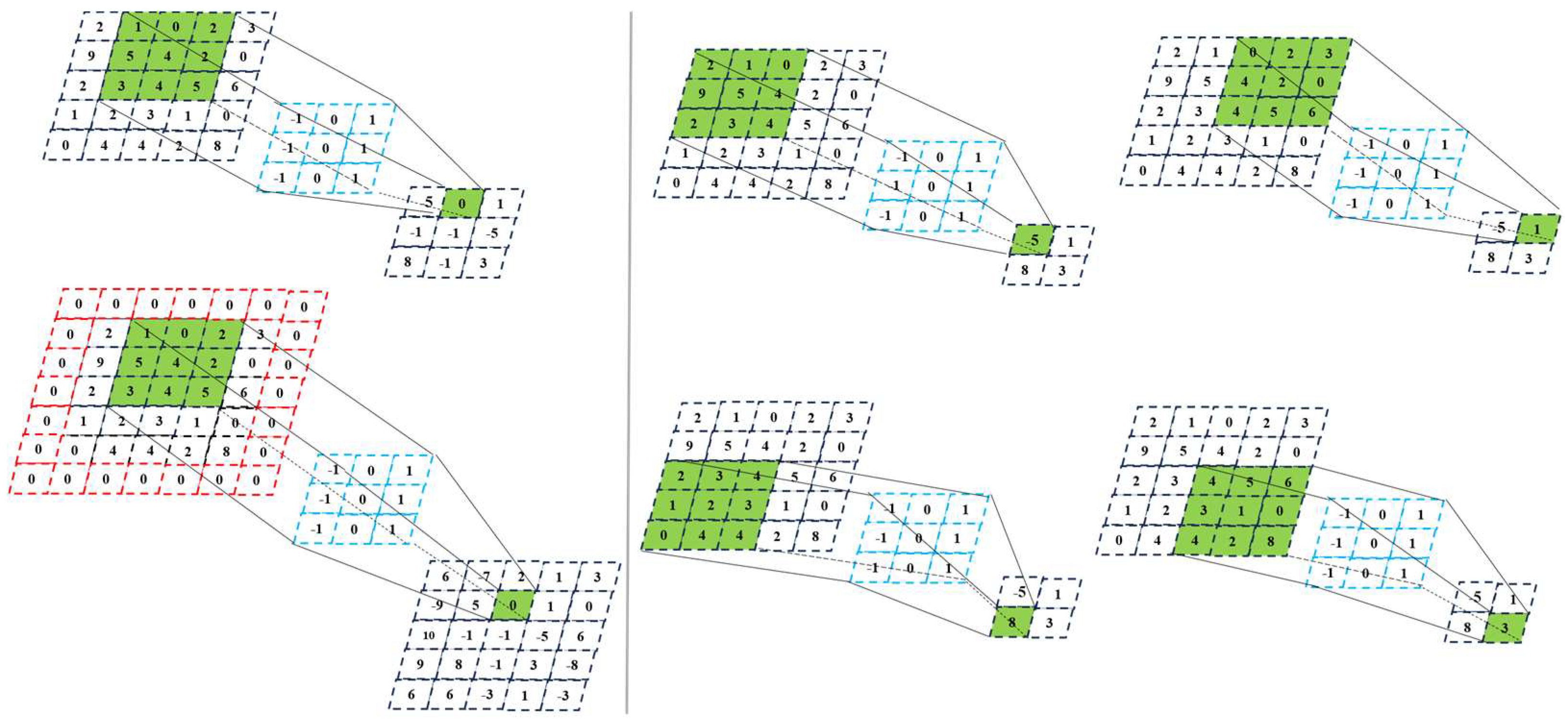
The convolutional layer is primarily used for feature extraction. The weights of the convolutional kernels are learnable, and their characteristic of ”parameter sharing” significantly reduces the network parameters, ensuring network sparsity. During computation, a matrix, also known as a convolutional kernel, is provided. The size of this matrix, also referred to as the receptive field, matches the depth of the input layer. Convolutional kernels of various depths form a filter with dimensions . To maintain the dimensional consistency after convolution operations, zero-padding, denoted as P, can be applied around the input matrix. During convolution, the kernel moves across the input matrix with a stride, denoted as S. Figure 2 is the schematic of the convolution operation when P = 1 & S = 2.
The formula for calculating the output features after the convolution operation is
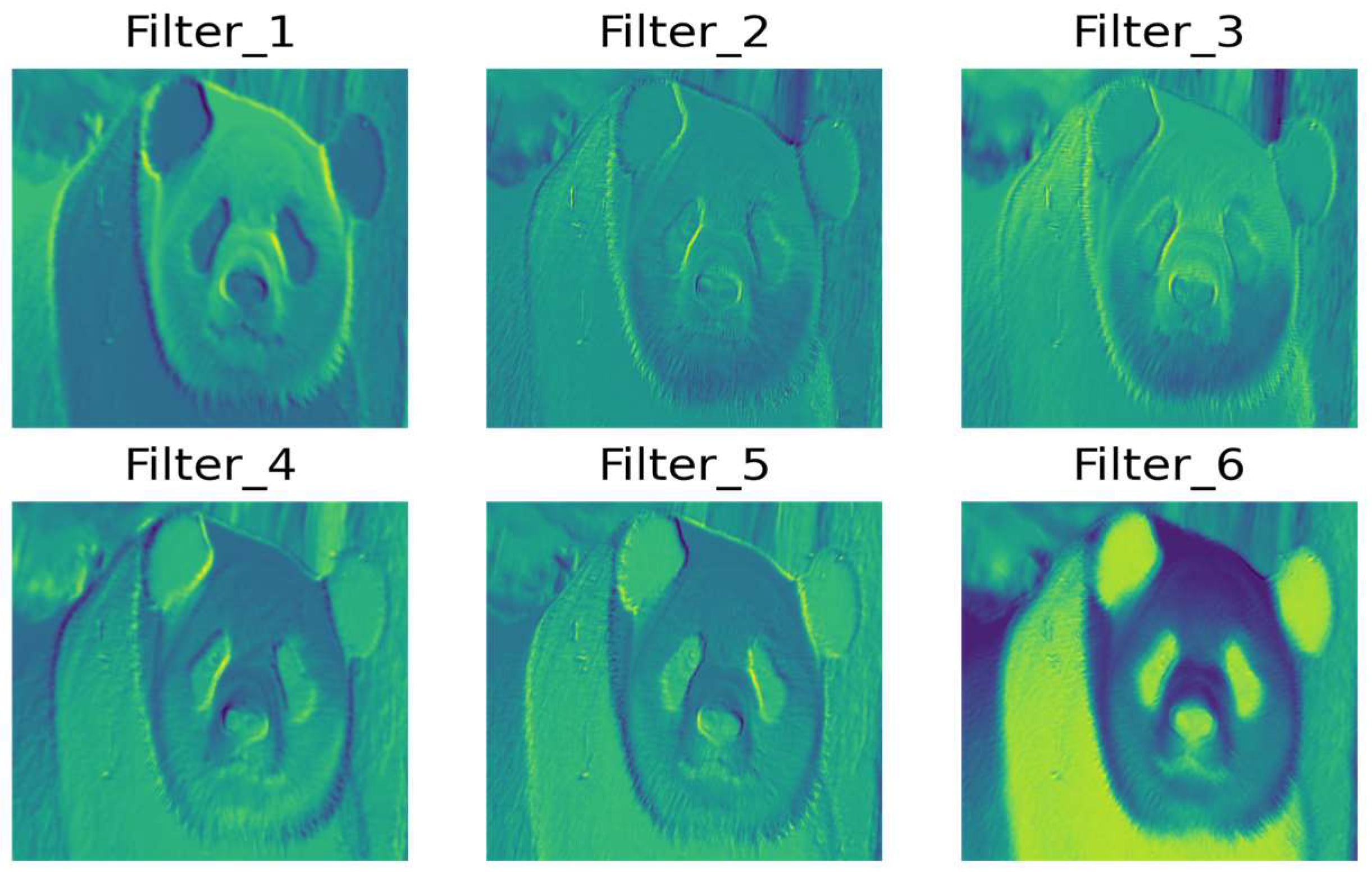
where is the dimension of the input features; represents the size of the convolutional kernel; and and denote the values for padding and stride, respectively. To visually demonstrate the effect of the convolutional layer, a 256 × 256-pixel image with three channels of a panda was randomly selected for the convolution operation, with a kernel size of 3 × 3 and six filters. The overall convolution effect and the effect of a single filter are shown in Figure 3 and Figure 4, respectively.
Figure 3 shows the comparative effects between the original image and the convolved image, with P = 0 and S = 1, resulting in output image dimensions of 252 × 252 and a channel count of six. In the convolution process, individual filters highlight different aspects of the image. Figure 4 demonstrates the convolution effect of a single filter, revealing that the output images from each filter are distinct. The collective outputs of all filters constitute the final output of the convolution layer.
2.2. MCP Regression and Solution
The standard linear regression model is as follows:
In the equation above, and represent the model’s intercept and coefficients, respectively, while denotes the total number of samples. Here, is the response variable of the sample, and is the predictor variable of the sample. In contrast to the least squares estimation (LSE) of the model, Lasso estimation incorporates L1 regularization into the loss function to strike a balance between model fitting and model complexity. The functional form of traditional Lasso regression is expressed as follows:
The regularization parameter, , is employed to control model complexity, reducing the model’s parameters by penalizing the sum of the absolute values of the coefficients, thereby encouraging a preference for model simplicity. Through the application of L1 regularization, the coefficients are reduced toward zero, leading to the elimination of redundant features. The Lasso penalty function, being convex and inducing biased estimation, mitigates the overall prediction error by reducing the variance in the prediction model. However, it is susceptible to the drawback of excessively compressing the coefficients. In pursuit of further minimizing the total prediction error, Fan and Li [40] introduced the SCAD penalty. This penalty not only compresses very small regression coefficients to zero but also provides an approximately unbiased estimation. Zhang [41] evidenced the Minimax Concave Penalty (MCP) as another notable penalty, validating its significance in the field. It differentiates penalties on regression coefficients, preserving the advantages of the SCAD penalty while yielding more precise estimates. The functional form of MCP regression is expressed as follows:
The variable is characterized by the following functional form:
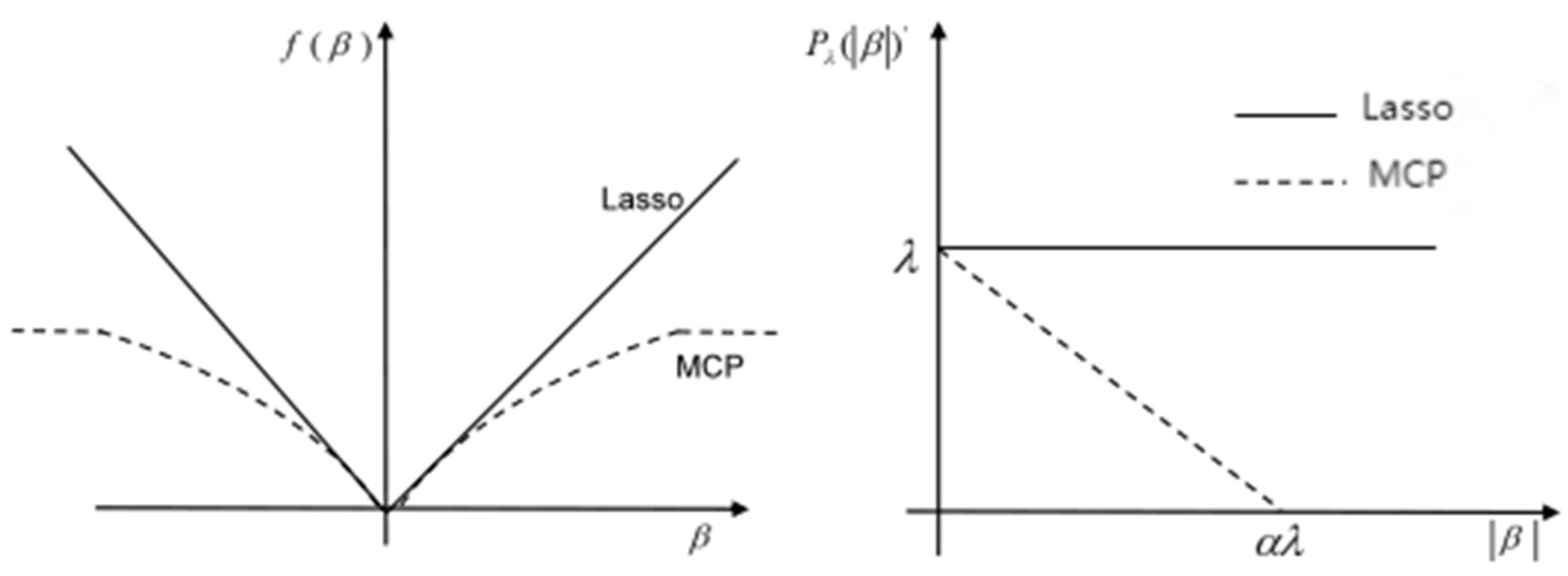
In the given equation, serves as the regularization parameter, employed to fine-tune the strength of the penalty, while functions as the adjustment parameter, regulating the extent of the penalty. The penalty strength can be expressed as follows:
In the above equation, denotes the penalty function. When , the MCP penalty diminishes as the absolute value of the parameter increases. At , the penalty reaches its maximum, , and when , the penalty becomes zero. As the regression coefficients continue to increase, the penalty remains unchanged at zero. In contrast, Lasso imposes a constant penalty on regression coefficients, while MCP applies variable penalties. Consequently, MCP yields more accurate coefficient fittings. When , MCP’s penalty strength is also zero, and its parameters are estimated similarly to least squares estimation. Figure 5 shows the difference between MCP and Lasso.
Common optimization algorithms, like gradient descent, are primarily designed for convex functions. However, the MCP penalty, being a sparse function, precludes the use of conventional gradient optimization algorithms. The coordinate descent algorithm is as follows:
For a differentiable convex function , where is n-dimensional, the goal of optimization is to iteratively decrease the loss function along the n coordinate axes (in the vector directions) of . When convergence is reached for each coordinate, , the loss function is minimized, and the corresponding is the solution. The computational steps are as follows:
- Randomly assign an initial value to the vector , denoted as .
- In the k-th round of iteration, compute each from to in sequence.
- Examine the variations in and in each dimension. If the change in all dimensions is less than a threshold, then is the final result; if not, proceed back to step 2 and carry on to the (k + 1)-th round of iteration.
The coordinate descent algorithm is a non-gradient optimization algorithm that cyclically uses different coordinate directions for iteration. One cycle of one-dimensional search iteration is equivalent to one iteration of gradient descent. It solves local optimization by fixing the other variables and optimizing along one direction at a time. Specifically, in the iterative solving process for p-dimensional features, , the other variables are held constant at their most recently updated values. Consequently, MCP regression can be viewed as optimized through a univariate solution scheme.
In the context of simple linear regression, the least squares solution employing the unpunished function is represented by , where denotes the normalized , resulting in . In MCP regression,
The variable represents the univariate solution derived from Lasso regression and is expressed as
From the aforementioned equation, the solutions of MCP regression and Lasso regression coincide when . The univariate solution of MCP is attained through the coordinate descent algorithm, aiming to minimize the coordinates of the objective function. The symbol is introduced to denote the remaining portion of column after removing its elements, and the partial residual of is represented by , where denotes the most recently updated value of . The MCP methodology is rooted in the coordinate descent algorithm; thus, the regression update step of MCP, based on the coordinate descent algorithm, can be expressed as
- (1)
- Calculate
- (2)
- Update
- (3)
- Update
2.3. Pruning Process
Figure 6 shows the specific pruning process. As illustrated below, channel pruning of a single convolutional layer is implemented to reduce the width of feature map B whilst maintaining the output quality of feature map C. Specifically, once channels in feature map B have been pruned, the corresponding filter channels—denoted by the dashed lines in W—can be eliminated. Similarly, the filters that generate these channels, indicated by the dashed lines from feature maps A to B, are also removable. The channel pruning process comprises two main steps: The first is channel selection, where the Maximal Channel Pruning (MCP) regression method is employed to discard redundant channels, retaining only those that are representative. The second step is the reconstruction of the output, achieved through linear regression to restore or reconstruct the output of the remaining channels, thereby ensuring that the network performance is unaffected by pruning. Through this process, although the width of feature map B is diminished, the output of feature map C is consistently preserved. The use of identical colors for blocks A and C represents the corresponding layers before and after compression, consistently maintaining the final output dimensions.
2.4. Preliminary Investigation of Convolutional Layer Parameters
Figure 7 is a scatter plot of the parameter distribution in the convolutional layers of the VGG19 network trained on the CIFAR100 dataset. For the VGG19 network with convolutional layers with 64, 128, 256, and 512 filters and for Layer1, Layer2, Layer3, and Layer4 in ResNet34, the quantiles are set at 0.99, 0.999, 0.9999, and 0.9999, respectively.
Figure 7 reveals that the distribution of parameters is mostly concentrated near zero, as indicated by the blue area, yet there are many points that are far from the center, represented by the red area. Using the L1-Norm method to measure the importance of filters may not be accurate. In the field of statistics, the Minimax Concave Penalty (MCP) introduces differentiated penalties for coefficients. When the absolute value of parameters exceeds a threshold, all parameters are replaced with a fixed value, and when the absolute value is below the threshold, different degrees of penalty are applied based on their magnitude. Zheng (2019) [42] noted that in the presence of tail errors or outliers, sparse penalties can lead to more accurate and robust models. Sun (2021) [43] discussed the selection problem when variables have outliers and applied the MCP penalty to logistic regression models, using a weighted method to mitigate the impact of outliers. Building on these findings, this study incorporates the MCP function into filter pruning to address the issue of ”outliers” in parameters. For parameters whose absolute values are above the threshold, they are considered equally important, and for those below the threshold, different degrees of compression are applied according to their magnitude, ensuring that larger parameters remain more significant while reducing the influence of “outliers” on filter importance. The expression for the MCP function is
In the above formula, is the regularization parameter, used to adjust the intensity of the penalty; is the tuning parameter, which controls the penalty range. To intuitively describe the effect of the MCP function, 100,000 weight parameters were randomly generated, with values in a range of [−1, 1]. Figure 8 depicts the results of the weight parameters after MCP processing under different and values.
When is fixed and is gradually increased, observing each row in the above figure, as increases, the range of the MCP function’s effect becomes larger, meaning the opening of the graph widens. Conversely, when is fixed and is gradually increased, observing each column in the figure, as increases, the penalty on values near zero becomes more severe, compressing values near zero to zero, resulting in a wider opening in the graph.
2.4.1. Description of Data Generation
In this study, the pruning of the convolutional layer is approached from both input and output perspectives. For each convolutional layer earmarked for pruning, it is essential to preserve both the input and output of the data. He [27] evidenced a methodology that considers the scale of the training data, adopting 2000 images as samples for model compression, validating the approach’s significance in the field. To achieve this, each image’s data are fed into the trained network, and the intermediate output of the model is retained for sampling. When pruning the feature map of a layer with channels, a matrix, , of size is sampled from the input feature map of the layer. Correspondingly, a matrix, , of size is generated from the output features, where N signifies the number of samples; n represents the number of output channels; and and denote the convolution sizes. For the sake of representation convenience, the bias term is not considered. The optimization function during pruning is
In the given equation, represents the matrix of the channel of after data transformation, with dimensions of . Similarly, denotes the channel of the data transformation of the weight earmarked for pruning, having dimensions of . In this context, and denote the intermediate inputs generated by the selected pruning samples through the trained network. Specifically, signifies the input of the current convolutional layer; represents the output of the current convolutional layer; and stands for the parameter of the convolutional layer, already trained at the current layer.
2.4.2. Channel Selection
Equation (12) is expressed as follows, where signifies the coefficient of the channel. The value of determines whether the channel is retained or not. When the value is 0, it indicates that this channel is not crucial for the output, and consequently, it is subject to pruning. Conversely, when the value is not 0, it signifies that this channel holds importance for the output and should not be cropped. In other words, the assessment of channel importance is contingent on the value of . During this scenario, the parameter in the model can be considered fixed, resulting in the formulation of Equation (9) in the subsequent manner:
The equation holds, with the dimensionality defined as .
2.4.3. Reconstruction of Outputs
Upon completion of channel selection, the coefficients, , associated with each channel are considered to be known. The parameters, , within the model can then be reconstructed by minimizing the mean square error. The optimization objective function is formulated as follows:
where , with dimensions of ; is the matrix of the transformed dimensions of the original parameters of the model with dimensions of ; and , with dimensions . The new model parameters, , can be reduced after solving for .
2.4.4. Parameter Selection
Throughout the training process, it is recommended to set parameter to 3 [39]. As for parameter , an initial value of is employed. The value of is incrementally increased until the count of remaining channels post-model pruning becomes lower than the initially specified number of channels to be retained. Subsequently, is determined through dichotomization until the remaining channels after pruning fall within the predefined range. Figure 9 illustrates a flowchart for parameter selection.
Algorithm 1 presents the pseudocode for parameter selection, where and represent the MCP parameters. The specified tolerance, , indicating the permissible number of channels within specific interval ranges post-model pruning, is set at 0.02 in our experiments. For instance, when configuring a pruning ratio of 0.1, the actual channel pruning ratio is considered to reach the threshold of 0.1 within a range of 0.098 to 0.12.
| Algorithm 1. Pseudocode for parameter selection. (# indicates an annotation on this line of pseudocode) |
| Inputs: Pruning ratio, MCP parameters , tolerance , current channel number c |
| Output: Reserved channels |
 |
3. Comparison Experiment
Ablation experiments were conducted on three networks, VGG19_Simple, VGG19, and ResNet34, using two datasets, CIFAR10 and CIFAR100. The VGG19_Simple model was employed, where the three fully connected layers in the original VGG19 model were reduced to two layers. The parameters of the original 4096 hidden layer neurons were adjusted to 512, significantly reducing the fully connected layer parameters. The VGG19 model, initially designed for the ImageNet dataset with 1000 categories, was adapted in our experiments to classify 100 categories. The training epoch for all models was set to 300. As ResNet34 was initially designed for the ImageNet dataset, its original input dimensions were 224 × 224. In the experiment using CIFAR100 with input dimensions of 32 × 32, adjustments were made to the first convolutional layer’s kernel size from 7 × 7 to 3 × 3. The learning rate for retraining was uniformly set at 0.001, with 40 epochs for the VGG model and 20 epochs for the ResNet34 model. The Top1 accuracy after MCP-L1 and L1-Norm pruning represents the average value of three repetitions.
He [28] demonstrated that the latter layers of the VGG model contain comparatively less information. Considering that the dimensions of the model’s input data are already reduced significantly by preceding pooling layers, and the computational requirements for these layers are notably lower than those of earlier convolutional layers, pruning the last few layers has a limited impact on overall computation reduction. Consequently, in the ablation experiments involving the VGG19_Simple and VGG19 models, the number of channels in the last four convolutional layers remains unchanged; in other words, no pruning is applied to these final four layers. Unlike employing distinct pruning ratios for varying filter quantities, our approach uses global ratios across all parameter-clipped layers, ensuring consistent ratios for all layers subjected to pruning.
3.1. Comparative Experiments with the VGG19_Simple Model
The experiments in this section involve the VGG19_Simple model, a variant of the original VGG19 model. In this modification, the three layers of full connectivity in VGG19 are consolidated into two layers, and the parameters of the initial 4096 hidden layer neurons are adjusted to 512. Following training on the CIFAR10 dataset, the achieved Top1 accuracy for the model is 92.7%. The corresponding floating-point computations amount to 3.99 × 10⁸, with a total of 2.03 × 10⁷ covariates.
3.1.1. Single-Layer Pruning Analysis
The reduction in Top1 accuracy for various layers was individually analyzed under three distinct methods: MCP-L1, Lasso regression, and MCP regression. This analysis was conducted based on different pruning ratios.
Figure 10 illustrates the impact of individual pruning on the 3rd to 11th convolutional layers in the VGG19_Simple model. The vertical axis represents the decrease in Top1 accuracy, where smaller values indicate superior performance. The horizontal axis denotes the specified pruning ratio, with 0.1 indicating a 10% reduction in the current channel. Observing the figure, minimal differences in Top1 accuracy reduction are noted among the three methods when the pruning ratio is small (i.e., 0.1). However, as the pruning ratio increases, all three curves exhibit an upward trend. Notably, the MCP-L1 curve exhibits the steepest ascent, followed by the Lasso regression curve, while the MCP regression curve demonstrates a more gradual increase. In instances of single-layer pruning, the MCP regression method excels in the selection of representative channels during pruning and in effectively reconstructing the output.
3.1.2. Global Pruning Analysis
For the VGG19_Simple model, we compared the Top1 accuracy of the model after pruning using three distinct compression methods, MCP-L1, Lasso regression, and MCP regression, across various pruning ratios. The pruned model underwent retraining at a pruning ratio of 0.3, with a training epoch of 40 and a learning rate of 0.001.
The results presented in Table 1 and Figure 11 illustrate distinct behaviors among three pruning methods: MCP-L1, Lasso regression, and MCP regression. MCP-L1 solely engages in channel pruning without output reconstruction. As the pruning ratio escalates, the model’s effectiveness diminishes significantly. When the pruning ratio reaches 0.5, the Top1 accuracy on CIFAR10 drops to a mere 11.61%, akin to random classification, rendering the model nearly ineffective. Lasso regression, coupled with output reconstruction, manages to maintain a relatively high accuracy rate. However, as the pruning ratio increases, its Top1 accuracy experiences a more rapid decline. In contrast, MCP regression, encompassing channel pruning along with output reconstruction, exhibits superior performance compared with the other two methods. A closer inspection of the local zoomed-in graph in Figure 3 underscores that, as the pruning proportion rises, the performance gap between Lasso regression and MCP regression widens progressively.
The insights derived from Table 2 reveal the substantial advantages of the MCP regression method in model pruning. When the pruning ratio is set to 0.1, the model demonstrates a commendable reduction of 15% in floating-point computation, accompanied by an 8% decline in the number of parameters. Remarkably, the Top1 accuracy of the pruned MCP regression model experiences only a marginal 1% decrease compared with the original model. Upon setting a pruning ratio of 0.4, the Top1 accuracy registers a modest decline of 2.5%, while the reduction in floating-point computation surpasses 50%. Correspondingly, the number of parameters decreases by over 30%, leading to an overall memory usage that is merely 70% of the original model. These results underscore the efficiency of the MCP regression method, as it achieves a balance between computational efficiency and model accuracy. In Table 2, with a pruning ratio of 0.3 and subsequent retraining, the MCP regression model showcases performance closer to the original model compared with other methods.
3.2. Comparative Experiments with the VGG19 Model
In contrast to the ablation experiment conducted on VGG19_Simple, modifications were made in the ablation experiment involving VGG19 to mitigate the impact of the fully connected layer on the pruning process. Specifically, the neurons in the last fully connected layer of the model were adjusted to 512, and the hidden layer with the largest parameter was downsized. This adjustment ensures that the majority of the model’s parameters and information are concentrated within the convolutional layer. An additional analysis was performed on the original VGG19 model concerning the pruning process. Given that the training dataset is CIFAR100, and the final classification number is 100, the Top1 accuracy of the model, after training on the CIFAR100 dataset, is 71.69%. The floating-point computation amounts to 4.18 × 10⁸, and the number of parameters is 3.93 × 10⁷.
3.2.1. Single-Layer Pruning Analysis
Similar to Figure 10, Figure 12 depicts the impact of individually pruning layers 3 to 11 of the convolutional layers in the VGG19 model trained using the CIFAR100 dataset. The vertical axis represents the decrease in Top1 accuracy, with smaller values indicating better performance. The horizontal axis denotes the specified pruning ratio, where 0.1 corresponds to pruning 10% of the current channel.
Redundancy exists in the VGG19 model trained on the CIFAR100 dataset, and pruning a certain percentage of channels leads to improved Top1 accuracy compared with the original network. In Figure 12a, when the pruning ratio is set to 0.15, 0.2, and 0.25, the MCP regression method enhances the Top1 accuracy by 0.02%, 0.11%, and 0.04%, respectively, upon pruning the model. In Figure 12b, at a pruning ratio of 0.1, both MCP regression and Lasso regression improve the accuracy by 0.13% and 0.08%, respectively. Figure 12i exhibits the most prominent redundancy phenomenon. At a pruning ratio of 0.1, when using MCP-L1 to directly crop the model, the accuracy improves by 0.15%. At this point, the MCP regression and Lasso regression methods are less effective than MCP-L1, although they also enhance the model’s performance after pruning.
In its entirety, the direct pruning of the model using the MCP-L1 method significantly diminishes the model’s performance, with a Top1 accuracy reduction exceeding 10% in shallower convolutional layers at a pruning ratio of 0.4. In contrast, MCP regression and Lasso regression involve an output reconstruction process, resulting in a more moderate degradation of the model’s performance compared with the MCP-L1 method. Notably, the MCP regression method outperforms Lasso regression in most cases, particularly in the middle layer of the network. At this layer, with fewer redundant parameters and more informative channels, channel selection becomes crucial. Consequently, the performance loss of the model after MCP regression is considerably smaller than that observed with the Lasso regression in Figure 12e–g.
3.2.2. Global Pruning Analysis
The Top1 accuracy after global model pruning was evaluated for the VGG19 model using three methods: MCP-L1, Lasso regression, and MCP regression. The model was retrained with a pruning ratio of 0.3, an epoch of 20, and a learning rate of 0.001.
As evident from Table 3 and Figure 13, the VGG19 model trained on CIFAR100 exhibits less parameter redundancy than VGG19_Simple trained on CIFAR10. Consequently, the decreases in Top1 accuracy are more pronounced when pruning the model.
When the model undergoes pruning using the MCP-L1 method, the Top1 accuracy experiences a significant drop, ranging from 20.54% to 51.15%, at a pruning ratio of 0.1. Upon reaching a pruning ratio of 0.5, the Top1 accuracy plummets to approximately 1%, rendering the model ineffective for a 100-category classification, akin to random classification. In the case of Lasso regression and MCP regression, although the decline in model performance is not as rapid as with the MCP-L1 method, the predictive effect diminishes notably with increasing pruning ratios. Specifically, at a pruning ratio of 0.5, the Top1 accuracies for the Lasso-regression- and MCP-regression-cropped models are 11.69% and 27.21%, representing 60% and 44.48% decreases, respectively.
Overall, the MCP regression method outperforms Lasso regression both after pruning the model and following fine-tuning. Specifically, at a pruning ratio of 0.3, the Top1 accuracies after pruning are 59.31% and 51.34% for MCP regression and Lasso regression, respectively. Subsequent retraining results in Top1 accuracies of 69.64% and 67.94%, with MCP regression exhibiting superior performance in both scenarios.
Table 4 displays the parametric quantities and floating-point computations of the VGG19 model with different pruning ratios. In the VGG19 model, a significant number of parameters are attributed to the fully connected layer, whereas a considerable portion of floating-point computations are concentrated in the convolutional layer. In this subsection’s experiments, pruning predominantly targets the convolutional channels, excluding the fully connected layer. Consequently, the reduction in the number of parameters after pruning is not pronounced, but the decline in floating-point computations is more substantial. For a pruning ratio of 0.5, the parameter count decreases by approximately 18%, while the floating-point computation volume drops by over 60%, resulting in a computation volume of less than half of the original model. With a pruning ratio of 0.3, the model’s Top1 accuracy is restored to 69.64% after only 40 retrains, representing a 2.05% reduction compared with the original model, accompanied by a reduction of about 42% in computation volume.
3.3. Comparative Experiments with ResNet34 Models
ResNet34, characterized by its multipath structure with residual elements, is designed for high efficiency and accuracy, making network tailoring more challenging. Similar to the VGG model, the floating-point computation of ResNet34 progressively decreases with each residual block as the depth increases, owing to pooling layers and a convolutional step size of two. In this section, inspired by ablation experiments on the VGG19_Simple and VGG19 models, we selectively crop the shallower layers of ResNet34—specifically, the convolutional layers in Layer1, Layer2, and Layer3, as detailed in the structure of ResNet34 in Table 2 and Table 3. Layer4’s computation amount decreases significantly due to its small output data, making it less significant for pruning compared with previous convolutional layers. The Top1 accuracy of the model trained on CIFAR100 data is 78.53%, with a floating-point computation of 1.16× 10⁹ and 2.13 × 10⁷ parameters.
3.3.1. Single-Layer Pruning Analysis
During single-layer pruning, strategy A excludes the pruning of residual branches, while strategy B involves pruning shortcuts and the Conv2 structure of Basic Block to maintain dimensionality consistency. In the single-layer pruning analysis, analysis was exclusively conducted to prune strategy A.
Figure 14 illustrates the single-layer pruning analysis for the first three Basic Blocks in Layer1 and Layer2 of the ResNet34 model. When applying single-layer pruning to the model in Layer1, the Top1 accuracy exhibits varying degrees of decrease. Notably, Basic Block1 experiences a less pronounced decrease, with MCP-L1 showing only a 0.4% reduction at a pruning ratio of 0.4. In contrast, Basic Block2 and Basic Block3 show more significant reductions of approximately 5% and 6% with the MCP-L1 method. Both the Lasso regression and MCP regression methods exhibit less-substantial decreases under single-layer pruning, with MCP regression demonstrating a slight superiority over Lasso regression methods.
In Layer2, none of the three methods exhibit a loss in Top1 accuracy at a given pruning ratio. This suggests redundancy in the ResNet34 model under CIFAR100 training, and pruning a single layer does not impact its performance. The Top1 accuracy also remains constant when pruning deeper Basic Blocks.
3.3.2. Global Pruning Analysis
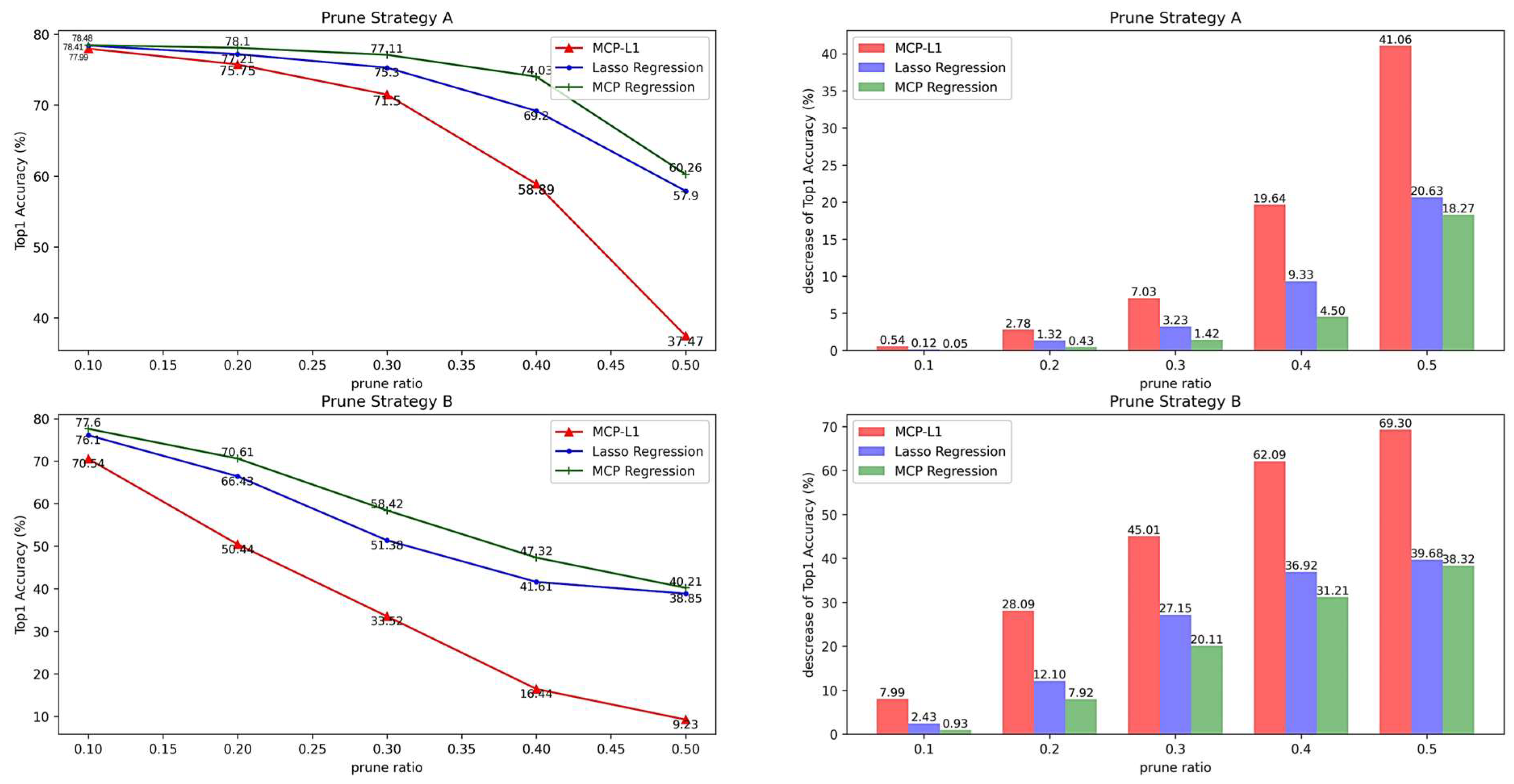
Table 5 and Figure 15 elucidate the repercussions of the three pruning methodologies subsequent to the global pruning of ResNet34, executed under two distinct pruning strategies. The left panels delineate the Top1 accuracy of the pruned model, while the right panels elucidate the magnitude of reduction in Top1 accuracy relative to that of the original model.
In strategy A, shortcut pruning is omitted, and the pruning process solely considers the number of channels in Conv1. With a pruning ratio of 0.1, the model’s performance only experiences a marginal decline across all three methods. However, as the pruning ratio escalates, there is a continuous deterioration in the model’s performance. Initially, the Top1 accuracy exhibits a gradual decrease; specifically, with a pruning ratio ranging from 0.1 to 0.3, the Top1 accuracies decrease by 6.49%, 1.2%, and 1.37% for the MCP-L1, Lasso regression, and MCP regression methods, respectively. Subsequently, from 0.3 to 0.5, the Top1 accuracies decrease by 34.03%, 17.38%, and 16.85%, respectively, for the three methods. As the pruning ratio increases, the model’s redundancy becomes insufficient to counterbalance the impact of channel pruning, resulting in a rapid performance decline. Among the three methods, Lasso regression and MCP exhibit smoother decline curves due to a more extensive output reconstruction process than MCP-L1. Notably, the MCP curve demonstrates the smoothest decline in Top1 accuracy.
In strategy B, incorporating shortcut pruning necessitates the simultaneous pruning of Conv2 in each Basic Block to maintain consistent output dimensions. Consequently, under identical pruning ratios, more information is pruned compared with strategy A. The graph illustrates a rapid decline in the model’s Top1 accuracy with increasing pruning ratios, forming an almost linear trend. Notably, the model’s Top1 accuracy experiences a swift, near-linear descent as the pruning ratio rises. This phenomenon can be attributed to the need to preserve information flow through the residual structure to prevent gradient vanishing. Consequently, the information loss in residual pruning surpasses that in the normal convolutional layer within the Basic Block. With a pruning ratio of 0.5, the Top1 accuracy of the model pruned using the MCP-L1 method plummets to below 10%, rendering the model nearly ineffective.
Under two distinct pruning strategies, the three pruning methods exhibited varying degrees of model performance degradation following the pruning of the ResNet34 model. Regardless of the strategy employed, the MCP regression method consistently outperformed the other two methods in pruning, suggesting its superior ability to select pruning channels compared with Lasso regression.
The data in Table 6 reveal insights into floating-point computations and parameter counts after pruning. The decrease in parameters is not pronounced under the two pruning strategies since channel pruning is limited to the convolutional layer. However, a substantial reduction in floating-point computations can be observed. At a pruning ratio of 0.1, the parameter reduction is approximately 3% to 4% for both strategies, while floating-point computation experiences a reduction exceeding 30%, nearly tenfold that of the parameter reduction. In strategy A, at a pruning ratio of 0.4, parameter reduction is merely 15%, but the corresponding reduction in floating-point computation exceeds 51%, less than half of the original model’s computation. For strategy B, with a pruning ratio of 0.5, floating-point computation is halved, while the parameter count shows a reduction of about 20%.
Strategy B not only prunes Conv2 in the Basic Block but also involves pruning the residual structure, resulting in a greater reduction in its parameter count compared with strategy A with the same pruning ratio. Nevertheless, the primary purpose of the residual structure is information conveyance and mitigating gradient vanishing effects, leading to a less pronounced decrease in floating-point computation when the residual structure is pruned. Under identical pruning ratios, although strategy B exhibits a larger parameter reduction, the decrease in floating-point computation is smaller than that of strategy A. Additionally, the floating-point computation in strategy A is less than that of strategy B.
4. Comparison of Scenarios Applicable to the MCP Regression and MCP-L1 Methods
Within the context of the VGG19 model, the comparison assesses distinctions between MCP-L1 and MCP regression based on time consumption and space occupation, with the pruning parameter set to 0.3.
4.1. Time Dimension
Efficiency in model pruning is a crucial area of interest. This subsection evaluates the pruning efficiency of the two methods based on their time consumption during the pruning of convolutional layers. For comparative purposes, Table 7 presents data on the time needed to crop a single convolutional kernel layer. This measurement excludes data preparation and other time-consuming factors, with the unit standardized in seconds (s).
Within the MCP regression method, convolutional layer filters are pruned considering both inputs and outputs. Consequently, for the initial layer of the model, which receives raw data as inputs, pruning is unsuitable. Therefore, there are no available data on the time consumption of the MCP regression compression method under Conv_1.
When considering time consumption, the VGG19 model’s increasing depth correlates with an extended duration for MCP regression pruning. This elongation can be attributed to rising dimensions, requiring fitting through the coordinate descent method, thus increasing the fitting time for a single layer. Dichotomous parameter selection during fitting necessitates continuous adjustments to maintain the retained channel count within the pruning range, amplifying the number of iterations. The time required is more pronounced with larger sample sizes. In contrast, the MCP-L1 method performs fewer operations when pruning a single convolutional layer, resulting in relatively minor time consumption. Even in deeper layers of the convolutional structure, its time consumption remains below 1 s.
4.2. The Space Dimension
Concerns regarding resource consumption arise during model pruning. This subsection gauges the necessary memory resources by evaluating the volume of data processed during the pruning of convolutional layers for both methods. For comparative analysis, the data in Table 8 represent the dimensions of data that require processing when pruning a single convolutional kernel layer.
The outcomes presented in Table 8 reveal that, within the MCP regression method, regression fitting is applied to the current output feature channel. The channel is censored based on whether the coefficient is zero or not to facilitate the pruning of the corresponding filter. Consequently, the data in this method need to be transformed into a two-dimensional format. In contrast, MCP-L1 directly prunes the filter in terms of parameters, utilizing it directly within the filter’s four-dimensional data structure.
When considering the spatial dimension, the MCP regression method faces an escalating challenge as the VGG19 model deepens. The pruning of a single convolutional layer involves an increasing number of samples and higher data dimensions. The solution process incorporates matrix operations, leading to significant memory occupancy during pruning. With the growing number of selected samples for pruning, the dimensionality of the data becomes more demanding on hardware resources. In contrast, MCP-L1 solely prunes in the original parameters, resulting in a modest change in the data processing volume and smaller memory occupancy for the model.
The data delineated in Table 7 and Table 8 unequivocally demonstrate the augmented time and memory requirements of the MCP regression method compared with the MCP-L1 method, particularly when processing deeper network structures. As evidenced in Table 7, the MCP regression approach exhibits a notable increase in the time needed for single-layer pruning as the model depth intensifies. This is especially pronounced in deeper convolutional layers, where the time consumption for MCP regression substantially exceeds that of the MCP-L1 method. For instance, at the Conv_16 layer, the time required by MCP regression amounts to 270.149 s, in stark contrast to the mere 0.779 s necessitated by the MCP-L1 method. This significant difference primarily stems from the necessity of more complex fitting computations via the coordinate descent method at each layer within the MCP regression framework. Regarding spatial resource consumption, the data from Table 8 indicate that the MCP regression method entails transforming the data into a two-dimensional format for each layer processed, resulting in increased memory usage. Notably, at the Conv_16 layer, the data dimension handled by the MCP regression method reaches 1,376,256,512, far surpassing the 51,251,233 managed by the MCP-L1 method. This illustrates that the memory requirements for filter pruning in MCP regression are significantly higher than those for the MCP-L1 method.
To address these computational overheads, we propose several strategies: Firstly, enhancing the efficiency of the coordinate descent algorithm or employing parallel processing techniques could reduce the time required for single-layer pruning. Secondly, for memory consumption, the exploration of data compression techniques or the adoption of more effective memory management strategies during the pruning process is recommended. Additionally, future work could investigate the substitution of MCP with other sparse penalty functions like ElasticNet or SCAD, potentially improving computational efficiency while maintaining model accuracy.
5. Discussion
With the widespread adoption of high-performance GPUs in the field of deep learning, both large and deep models have surpassed human limits across various domains. The extensive use of billions, or even trillions, of parameters along with computationally intensive operations confines these models to operation solely within laboratories and data centers. The fundamental requirements for real-time online devices handling deep neural networks include high precision and low latency. Consequently, compressing and accelerating models have become crucial areas of research in academia and industry. The focus remains on how to downsize these large models to facilitate deployment on mobile devices, attracting significant attention.
He [28] was the pioneer in employing Lasso regression for model compression, removing redundant channels through this technique. In channel selection, Lasso applies a constant penalty strength to the regression coefficients. However, Lee and Kim [32] argued that optimizing penalized regression is simpler and more cost-effective than subset selection. Additionally, Xu and Lei [33] introduced sparsity to the original variables and incorporated sparse regression based on traditional principal component analysis. This not only retained the advantages of traditional principal component analysis but also enhanced model estimation accuracy due to its sparsity. Lin et al. [34] proposed a variable selection method for the functional regression model in the case of sparse functional-type data. They performed functional principal component analysis on sparse functional-type independent variables based on conditional expectation. The estimated orthogonal eigenfunctions were then used as basis functions to expand the model. In contrast to He, [28] evidences the application of MCP regression for channel selection, deviating from the use of Lasso regression. This modification, introducing the MCP regularization function, validates the work’s significance in this field. We also adhere to the use of maximum squares regression.
The global pruning analysis, encompassing the single-layer pruning of the model, demonstrated the superior performance of MCP regression over Lasso regression. Comparative experiments were conducted on two datasets, CIFAR10 and CIFAR100, involving three networks: VGG19_Simple, VGG19, and ResNet34. Specifically, for VGG19_Simple trained on the CIFAR10 dataset, the Top1 accuracy of the MCP regression method after pruning improved by an average of 2.3% compared with that of the Lasso regression method. Due to the smaller dataset and increased model redundancy, the accuracy of the model remained higher after pruning. For the VGG19 model trained on the CIFAR100 dataset, where model redundancy is relatively low, channel selection becomes crucial. Here, the Top1 accuracy of the model after MCP regression increased by an average of 10% compared with that of the Lasso method, and the accuracy of Top1 after retraining improved by 0.67% at a pruning ratio of 0.3. For the ResNet34 model trained on the CIFAR100 dataset, with less model redundancy than VGG19, the Top1 accuracies of the MCP method improved by an average of 1.98% and 4.56% compared with that of the Lasso method after Lasso method pruning under two different strategies. In summary, all three ablation experiments consistently demonstrated the superiority of MCP regression for channel selection followed by output reconstruction over Lasso regression for channel selection followed by reconstruction.
In the experimental section, it is evident that the MCP regression method yields a higher accuracy for the pruned model in comparison with MCP-L1. Additionally, the accuracy of the fine-tuned model approaches that of the original model. However, the computational time consumption and memory usage of the MCP regression method significantly surpass those of MCP-L1. Consequently, each method has its own set of advantages and disadvantages. When dealing with more complex problems, larger models, and an increased training data volume, it is preferable to utilize the MCP-L1 method for model pruning. Opting for the MCP regression method in such cases poses challenges. Given the particularly large volume of training data in the original model, maintaining effective pruning requires a correspondingly substantial selection of data during the pruning process. Consequently, the time consumption for model pruning becomes extensive, necessitating significant storage capacity in the hardware or clusters for implementation. In scenarios where the problem to be solved is relatively straightforward, and the model is not excessively large, employing MCP regression for model pruning is more advantageous. In contrast to MCP-L1, MCP regression pruning encompasses an output reconstruction phase, leading to higher accuracy. Particularly for models exhibiting substantial redundancy, there might be no necessity for retraining after direct pruning.
This study explores the application of the sparse penalty function MCP in tailoring convolutional neural networks. However, due to our limitations in capacity and time constraints, some envisioned ideas remain unrealized. There are still aspects to investigate in future work, including the following: (1) This study exclusively delves into the sparse penalty function MCP. However, other outstanding regression methods in the field of statistics, such as ElasticNet and SCAD, can also be applied to channel selection. (2) This study maintains a fixed pruning ratio to determine the number of channels for removal. The challenge lies in providing an optimal channel count directly through model perception or parameter selection. This approach ensures that the cropped model eliminates redundant parameters without sacrificing information, thereby obviating the necessity for retraining to fine-tune the model.
6. Conclusions
Model compression and acceleration have been the focal points of research in academia and industry. The endeavor to shrink large models for deployment on mobile devices has garnered significant attention. Simultaneously, considering the convolution process as a linear regression process and utilizing regression coefficients to discern channel redundancy are prominent avenues in current structured pruning. In the realm of statistics, Lasso regression serves as a common feature selection method. However, with the ascent of sparse penalty function research, regression based on the sparse penalty function is gradually eclipsing Lasso regression in the field of feature selection.
Building upon this foundation, we incorporate MCP regression into convolutional channel screening, coupled with coordinate descent, to facilitate the removal of redundant channels. For the remaining channels, we engage in reconstruction through the original least squares method. Comparative experiments are conducted on two datasets, CIFAR10 and CIFAR100, and three networks, VGG19_Simple, VGG19, and ResNet34. Notably, for VGG19_Simple trained on the CIFAR10 dataset, the MCP regression method demonstrates a 2.3% improvement in Top1 accuracy, on average, compared with the Lasso regression method. Despite the smaller dataset and greater model redundancy, the accuracy of the model remains higher after pruning. Conversely, in the VGG19 model trained on the CIFAR100 dataset, where model redundancy is comparatively small, channel selection becomes more critical. At this juncture, the Top1 accuracy of the model after MCP regression increases by an average of 10% compared with that of the Lasso method, and the accuracy of Top1 after retraining increases by 0.67% with a pruning ratio of 0.3. For the ResNet34 model trained on the CIFAR100 dataset, with less model redundancy than VGG19, the MCP method outperforms the Lasso method, with average improvements in Top1 accuracy of 1.98% and 4.56% after Lasso method pruning under two different strategies. In summary, all three ablation experiments underscore the superiority of the MCP regression method for channel selection followed by output reconstruction over Lasso regression. Thus, we conclude that MCP regression supersedes Lasso regression in achieving enhanced pruning.
Author Contributions
Methodology, L.Z.; Data curation, L.Z.; Writing—original draft, X.L.; Writing—review & editing, X.L.; Visualization, X.L.; Supervision, Y.L.; Project administration, Y.L.; Funding acquisition, Y.L. All authors have read and agreed to the published version of the manuscript.
Funding
This research was funded by National Social Science Fund of China grant number 17BJY210, by National Natural Science Foundation of China (11701161) and by Key Humanities and Social Science Fund of Hubei Provincial Department of Education (20D043).
Data Availability Statement
Public-ly available datasets were analyzed in this study. This data can be found here: [https://www.cs.toronto.edu/~kriz/cifar.html, accessed on 22 April 2024].
Conflicts of Interest
The authors declare no conflict of interest.
References
- Li, Y.L. Model Compression of Deep Neural Networks. Master’s Thesis, University of Electronic Science and Technology of China, Chengdu, China, 2022; pp. 1–6. [Google Scholar] [CrossRef]
- Xu, J.H. Research on Model Compression and Acceleration of Deep Neural Networks Based on Model Pruning. Master’s Thesis, Southeast University, Nanjing, China, 2020; pp. 1–7. [Google Scholar] [CrossRef]
- LeCun, Y.; Bottou, L.; Bengio, Y.; Haffner, P. Gradient-based learning applied to document recognition. Proc. IEEE 1998, 86, 2278–2324. [Google Scholar] [CrossRef]
- Zhang, K.Z.; Li, Y.W.; Liu, B.; Li, J.; Xie, H.; Zhang, Z.Y. Research on hyperparameter tuning strategies based on VGG16 network. Sci. Innov. 2021, 22, 10–13. [Google Scholar]
- Chen, W.J. Design and Implementation of a High-Speed and High-Precision Matrix Inverter. Master’s Thesis, Hefei University of Technology, Hefei, China, 2021. [Google Scholar]
- Mehbodniya, A.; Kumar, R.; Bedi, P.; Mohanty, S.N.; Tripathi, R.; Geetha, A. VLSI implementation using fully connected neural networks for energy consumption over neurons. Sustain. Energy Technol. Assess. 2022, 52, 102058. [Google Scholar] [CrossRef]
- Li, Z.; Li, H.Y.; Meng, L. Model compression for deep neural networks: A survey. Computers 2023, 12, 60. [Google Scholar] [CrossRef]
- Deng, L.; Li, G.Q.; Han, S.; Shi, L.; Xie, Y. Model compression and hardware acceleration for neural networks: A comprehensive survey. Proc. IEEE 2020, 108, 485–532. [Google Scholar] [CrossRef]
- Zhou, Y.; Xia, L.; Zhao, J.Q.; Yao, R.; Liu, B. Efficient convolutional neural networks and network compression methods for object detection: A survey. Multimed. Tools Appl. 2024, 83, 10167–10209. [Google Scholar] [CrossRef]
- Rokh, B.; Azarpeyvand, A.; Khanteymoori, A. A comprehensive survey on model quantization for deep neural networks in image classification. ACM Trans. Intell. Syst. Technol. 2023, 14, 1–50. [Google Scholar] [CrossRef]
- Geng, L.L.; Niu, B.N. A comprehensive review on model compression of deep neural networks. Comput. Sci. Explor. 2020, 14, 1441–1455. [Google Scholar]
- Si, Z.F.; Qi, H.G. A comprehensive review on knowledge distillation methods and applications. J. Chin. Soc. Image Graph. 2023, 28, 2817–2832. [Google Scholar]
- Hu, M.H.; Gao, R.B.; Suganthan, P.N. Self-Distillation for Randomized Neural Networks. In IEEE Transactions on Neural Networks and Learning Systems; IEEE: New York, NY, USA, 2023. [Google Scholar]
- Liu, X.; Wang, X.G.; Matwin, S. Improving the interpretability of deep neural networks with knowledge distillation. In Proceedings of the 2018 IEEE International Conference on Data Mining Workshops (ICDMW), Singapore, 17–20 November 2018; IEEE: New York, NY, USA, 2018; pp. 905–912. [Google Scholar]
- Zhang, L.F.; Bao, C.L.; Ma, K.S. Self-distillation: Towards efficient and compact neural networks. IEEE Trans. Pattern Anal. Mach. Intell. 2022, 44, 4388–4403. [Google Scholar] [CrossRef]
- Ning, X.; Zhao, W.Y.; Zong, Y.X.; Zhang, Y.G.; Chen, H.; Zhou, Q.; Ma, J.X. A comprehensive review on joint optimization methods for neural network compression. J. Intell. Syst. 2024, 1–21. [Google Scholar] [CrossRef]
- Chang, J.F. Research on Channel Pruning Methods for Deep Convolutional Neural Networks. Ph.D. Dissertation, Hefei University of Technology, Hefei, China, 2022. [Google Scholar]
- LeCun, Y.; Denker, J.; Solla, S. Optimal brain damage. In Proceedings of the Advances in Neural Information Processing Systems, San Francisco, CA, USA, 2 June 1990; pp. 598–605. [Google Scholar]
- Hassibi, B.; Stork, D.G. Second order derivatives for network pruning: Optimal brain surgeon. In Proceedings of the Advances in Neural Information Processing Systems, Denver, CO, USA, 29 November–2 December 1993; pp. 164–171. [Google Scholar]
- Wu, T.; Li, X.Y.; Zhou, D.Y.; Li, N.; Shi, J. Differential evolution based layer-wise weight pruning for compressing deep neural networks. Sensors 2021, 21, 880. [Google Scholar] [CrossRef] [PubMed]
- Xu, P.T.; Cao, J.; Sun, W.Y.; Li, P.; Wang, Y.; Zhang, X. Layer Pruning Method of Deep Neural Network Models Based on Mergeable Residual Convolutional Blocks. J. Peking Univ. (Nat. Sci. Ed.) 2022, 58, 801–807. [Google Scholar]
- Li, R.Q.; Zhu, L.; Liu, Y.Y. Filter elastic deep neural network channel pruning compression method. Comput. Eng. Appl. 2022, 32, 136–141. [Google Scholar]
- Zhang, J.Y.; Kou, J.Q.; Liu, N.Z. Neural network pruning algorithm based on filter distribution fitting. Comput. Technol. Dev. 2022, 32, 136–141. [Google Scholar]
- Geng, L.L.; Niu, B.N. Pruning convolutional neural networks via filter similarity analysis. Mach. Learn. 2022, 111, 3161–3180. [Google Scholar] [CrossRef]
- Chen, K.; Wang, A.Z. A review on regularization methods of convolutional neural networks. Comput. Appl. Res. 2024, 1–11. [Google Scholar] [CrossRef]
- Alemu, H.Z.; Wu, W.; Zhao, J.H. Feedforward neural networks with a hidden layer regularization method. Symmetry 2018, 10, 525. [Google Scholar] [CrossRef]
- Lin, Z.J.; Wang, J.K.; Xie, J.M.; Li, Z.; Xie, S. Dual-Strategy Structured Neural Network Compression with Unbiased Sparse Regularization. Inf. Control 2023, 52, 313–325. [Google Scholar]
- He, Y.; Zhang, X.; Sun, J. Channel pruning for accelerating very deep neural networks. In Proceedings of the IEEE International Conference on Computer Vision, Venice, Italy, 22–29 October 2017; pp. 1389–1397. [Google Scholar]
- Wang, L.; Sun, J.B. Application of Lasso Regression Method in Feature Variable Selection. J. Jilin Eng. Norm. Univ. 2021, 37, 109–112. [Google Scholar]
- Farbahari, A.; Dehesh, T.; Gozashti, M.H. The Usage of Lasso, Ridge, and Linear Regression to Explore the Most Influential Metabolic Variables that Affect Fasting Blood Sugar in Type 2 Diabetes Patients. Rom. J. Diabetes Nutr. Metab. Dis. 2019, 26, 371–379. [Google Scholar] [CrossRef]
- Wu, J.; Wu, H.N.; Liu, A.; Li, C.; Li, Q. A Deep Learning Model Compression Method Based on Lasso Regression and SVD Fusion. Telecommun. Technol. 2019, 59, 495–500. [Google Scholar]
- Lee, S.; Kim, S. Marginalized Lasso in Sparse Regression. J. Korean Stat. Soc. 2019, 48, 396–411. [Google Scholar] [CrossRef]
- Xu, J.L.; Lei, X.Y. Research on Variable Selection Based on Sparse Regression. J. Qilu Univ. Technol. 2022, 36, 75–80. [Google Scholar]
- Lin, S.F.; Yi, D.H.; Li, Y.; Li, J. Variable Selection and Empirical Analysis for Sparse Functional Regression Models. Math. Pract. Underst. 2016, 46, 171–177. [Google Scholar]
- Yoshida, T. Quantile Function Regression and Variable Selection for Sparse Models. Can. J. Stat. 2021, 49, 1196–1221. [Google Scholar] [CrossRef]
- Shin, J.K.; Bak, K.Y.; Koo, J.Y. Sparse Neural Network Regression with Variable Selection. Comput. Intell. 2022, 38, 2075–2094. [Google Scholar] [CrossRef]
- Zhou, L.; Luo, Y.X. Dual MCP Penalty Quantile Regression for Mixed-Effect Models. J. Cent. China Norm. Univ. (Nat. Sci.) 2021, 55, 991–999. [Google Scholar]
- Xue, X.Q.; Li, Y.; Liang, J.R. Functional Hypernetwork Analysis of the Human Brain and Depression Classification Based on Group MCP and Composite MCP. Small Micro Comput. Syst. 2022, 43, 210–217. [Google Scholar]
- Sun, H.W.; Yang, W.Y.; Wang, H.; Luo, W.H.; Hu, N.B.; Wang, T. Simulation Evaluation of Penalized Logistic Regression for High-Dimensional Variable Selection. Chin. Health Stat. 2016, 33, 607–611. [Google Scholar]
- Fan, J.; Li, R. Variable Selection via Nonconcave Penalized Likelihood and its Oracle Properties. J. Am. Stat. Assoc. 2001, 96, 1348–1360. [Google Scholar] [CrossRef]
- Zhang, C.H. Nearly unbiased variable selection under minimax concave penalty. Ann. Stat. 2010, 38, 894–942. [Google Scholar] [CrossRef] [PubMed]
- Zheng, W.H. Research on AdaBoost Ensemble Pruning Technique Based on MCP Penalty. Master’s Thesis, Jiangxi University of Finance and Economics, Nanchang, China, 2019. [Google Scholar]
- Sun, G.F.; Wang, M.Q. Robust Group Variable Selection in Logistic Regression Model. Stat. Decis. 2021, 37, 42–45. [Google Scholar]
Figure 1.
Computational flow of a single neuron and fully connected network.

Figure 2.
Schematic of convolution operation with P = 1 and S = 2.

Figure 3.
Convolution effect diagram.

Figure 4.
Effect diagram of a single filter.

Figure 5.
MCP and Lasso comparison diagram.

Figure 6.
Schematic diagram of the pruning process.

Figure 7.
VGG19 convolutional layer parameter distribution diagram. Blue represents weight values close to 0, red represents weight values a little further away from 0.
Figure 7.
VGG19 convolutional layer parameter distribution diagram. Blue represents weight values close to 0, red represents weight values a little further away from 0.

Figure 8.
Effect diagram of and parameter values.

Figure 9.
Parameter selection flowchart.

Figure 10.
VGG19_Simple single-layer pruning diagram.

Figure 11.
VGG19_Simple global pruning comparison chart.

Figure 12.
VGG19 single-layer pruning diagram. Subfigures(a–i) represent the results of pruning layers 3 to 11 respectively.
Figure 12.
VGG19 single-layer pruning diagram. Subfigures(a–i) represent the results of pruning layers 3 to 11 respectively.

Figure 13.
Comparison of the global pruning of VGG19.

Figure 14.
Schematic of ResNet34 single-layer pruning under strategy A.

Figure 15.
Global pruning effect of ResNet34.


Table 1.
Global pruning comparison diagram of VGG19_Simple.
| 0.1 | 0.2 | 0.3 | 0.4 | 0.5 | Retrain (0.3) | |
|---|---|---|---|---|---|---|
| MCP-L1 | 83.49 | 54.33 | 37.88 | 20.4 | 10.61 | 91.43 |
| Lasso Regression | 91.19 | 89.27 | 87.93 | 86.81 | 82.97 | 91.74 |
| MCP Regression | 91.7 | 91.37 | 90.55 | 90.13 | 88.62 | 91.95 |
Table 2.
Parameter counts and floating-point calculations of VGG19_Simple model with different pruning ratios.
Table 2.
Parameter counts and floating-point calculations of VGG19_Simple model with different pruning ratios.
| Ratio | Flop | Flop Ratio | Param | Param Ratio |
|---|---|---|---|---|
| 0.1 | 3.37 × 10⁸ | 15.52% | 1.86 × 10⁷ | 8.23% |
| 0.2 | 2.78 × 10⁸ | 30.25% | 1.70 × 10⁷ | 16.39% |
| 0.3 | 2.25 × 10⁸ | 43.75% | 1.55 × 10⁷ | 23.76% |
| 0.4 | 1.80 × 10⁸ | 54.94% | 1.42 × 10⁷ | 30.02% |
| 0.5 | 1.39 × 10⁸ | 64.99% | 1.30 × 10⁷ | 35.88% |
Table 3.
Table of VGG19 global pruning results.
| 0.1 | 0.2 | 0.3 | 0.4 | 0.5 | Retrain (0.3) | |
|---|---|---|---|---|---|---|
| MCP-L1 | 51.15 | 22.08 | 7.57 | 2.28 | 1.13 | 67.49 |
| Lasso Regression | 67.08 | 60.41 | 51.34 | 20.13 | 11.69 | 67.97 |
| MCP Regression | 70.06 | 66.11 | 59.31 | 45.92 | 27.21 | 69.64 |
Table 4.
Parametric quantities and floating-point computations of VGG19 model with different pruning ratios.
Table 4.
Parametric quantities and floating-point computations of VGG19 model with different pruning ratios.
| Ratio | Flop | Flop Ratio | Param | Param Ratio |
|---|---|---|---|---|
| 0.1 | 3.51 × 10⁸ | 15.86% | 3.75 × 10⁷ | 4.58% |
| 0.2 | 2.93 × 10⁸ | 29.82% | 3.59 × 10⁷ | 8.74% |
| 0.3 | 2.41 × 10⁸ | 42.32% | 3.44 × 10⁷ | 12.44% |
| 0.4 | 1.96 × 10⁸ | 53.20% | 3.31 × 10⁷ | 15.76% |
| 0.5 | 1.57 × 10⁸ | 62.32% | 3.20 × 10⁷ | 18.63% |
Table 5.
Plot of global pruning results for ResNet34.
| 0.1 | 0.2 | 0.3 | 0.4 | 0.5 | Retrain (0.3) | ||
|---|---|---|---|---|---|---|---|
| Pruning Strategy A | MCP-L1 | 77.99 | 75.57 | 71.50 | 58.89 | 37.47 | 76.94 |
| Lasso Regression | 78.41 | 77.21 | 75.30 | 69.20 | 57.92 | 77.34 | |
| MCP Regression | 78.48 | 78.10 | 77.11 | 74.03 | 60.26 | 77.67 | |
| Pruning Strategy B | MCP-L1 | 70.54 | 50.44 | 33.52 | 16.44 | 9.23 | 77.16 |
| Lasso Regression | 76.10 | 66.43 | 51.38 | 41.61 | 35.85 | 77.58 | |
| MCP Regression | 77.60 | 70.61 | 58.42 | 47.32 | 40.21 | 77.84 | |
Table 6.
Parameter count and floating-point computation of ResNet34 model with different pruning ratios.
Table 6.
Parameter count and floating-point computation of ResNet34 model with different pruning ratios.
| Ratio | Flop | Flop Ratio | Param | Param Ratio | |
|---|---|---|---|---|---|
| Prune Strategy A | 0.1 | 1.07 × 10⁹ | 33.46% | 2.05 × 10⁷ | 3.56% |
| 0.2 | 9.77 × 10⁸ | 39.31% | 1.97 × 10⁷ | 7.42% | |
| 0.3 | 8.81 × 10⁸ | 45.27% | 1.89 × 10⁷ | 11.17% | |
| 0.4 | 7.87 × 10⁸ | 51.11% | 1.81 × 10⁷ | 15.04% | |
| 0.5 | 6.89 × 10⁸ | 57.19% | 1.73 × 10⁷ | 18.92% | |
| Prune Strategy B | 0.1 | 1.09 × 10⁹ | 32.18% | 2.04 × 10⁷ | 4.06% |
| 0.2 | 1.02 × 10⁹ | 36.76% | 1.95 × 10⁷ | 8.44% | |
| 0.3 | 9.46 × 10⁹ | 41.23% | 1.86 × 10⁷ | 12.68% | |
| 0.4 | 8.73 × 10⁸ | 45.80% | 1.77 × 10⁷ | 17.06% | |
| 0.5 | 7.99 × 10⁸ | 50.37% | 1.67 × 10⁷ | 21.43% |
Table 7.
Comparison of time consumption of the two methods.
| Layer | MCP-L1 | MCP Regression | Layer | MCP-L1 | MCP Regression |
|---|---|---|---|---|---|
| Conv_1 | 0.029 | ---- | Conv_9 | 0.705 | 25.276 |
| Conv_2 | 0.077 | 2.315 | Conv_10 | 0.813 | 43.445 |
| Conv_3 | 0.068 | 2.674 | Conv_11 | 0.798 | 88.056 |
| Conv_4 | 0.189 | 2.220 | Conv_12 | 0.767 | 135.252 |
| Conv_5 | 0.256 | 5.096 | Conv_13 | 0.726 | 435.779 |
| Conv_6 | 0.495 | 8.199 | Conv_14 | 0.714 | 246.687 |
| Conv_7 | 0.496 | 6.750 | Conv_15 | 0.670 | 274.217 |
| Conv_8 | 0.493 | 9.415 | Conv_16 | 0.779 | 270.149 |
Table 8.
Table of dimensions of data cropped by the two methods.
| Layer | MCP-L1 | MCP Regression | Layer | MCP-L1 | MCP Regression |
|---|---|---|---|---|---|
| Conv_1 | (3,64,3,3) | ---- | Conv_9 | (256,512,3,3) | (1376256,256) |
| Conv_2 | (64,64,3,3) | (172032,64) | Conv_10 | (512,512,3,3) | (1376256,512) |
| Conv_3 | (64,128,3,3) | (344064,64) | Conv_11 | (512,512,3,3) | (1376256,512) |
| Conv_4 | (128,128,3,3) | (344064,128) | Conv_12 | (512,512,3,3) | (1376256,512) |
| Conv_5 | (128,256,3,3) | (688128,128) | Conv_13 | (512,512,3,3) | (1376256,512) |
| Conv_6 | (256,256,3,3) | (688128,256) | Conv_14 | (512,512,3,3) | (1376256,512) |
| Conv_7 | (256,256,3,3) | (688128,256) | Conv_15 | (512,512,3,3) | (1376256,512) |
| Conv_8 | (256,256,3,3) | (688128,256) | Conv_16 | (512,512,3,3) | (1376256,512) |
Disclaimer/Publisher’s Note: The statements, opinions and data contained in all publications are solely those of the individual author(s) and contributor(s) and not of MDPI and/or the editor(s). MDPI and/or the editor(s) disclaim responsibility for any injury to people or property resulting from any ideas, methods, instructions or products referred to in the content. |
© 2024 by the authors. Licensee MDPI, Basel, Switzerland. This article is an open access article distributed under the terms and conditions of the Creative Commons Attribution (CC BY) license (https://creativecommons.org/licenses/by/4.0/).
Share and Cite
MDPI and ACS Style
Liu, X.; Zhou, L.; Luo, Y. Pruning Deep Neural Network Models via Minimax Concave Penalty Regression. Appl. Sci. 2024, 14, 3669. https://0-doi-org.brum.beds.ac.uk/10.3390/app14093669
AMA Style
Liu X, Zhou L, Luo Y. Pruning Deep Neural Network Models via Minimax Concave Penalty Regression. Applied Sciences. 2024; 14(9):3669. https://0-doi-org.brum.beds.ac.uk/10.3390/app14093669
Chicago/Turabian StyleLiu, Xinggu, Lin Zhou, and Youxi Luo. 2024. "Pruning Deep Neural Network Models via Minimax Concave Penalty Regression" Applied Sciences 14, no. 9: 3669. https://0-doi-org.brum.beds.ac.uk/10.3390/app14093669
Note that from the first issue of 2016, this journal uses article numbers instead of page numbers. See further details here.