
A Novel Method for Anomaly Detection and Signal Calibration in Water Quality Monitoring of an Urban Water Supply System

Campus Ålesund, Norwegian University of Science and Technology, 6009 Ålesund, Norway
*
Author to whom correspondence should be addressed.
Water 2024, 16(9), 1238; https://0-doi-org.brum.beds.ac.uk/10.3390/w16091238
Submission received: 8 March 2024
/
Revised: 16 April 2024
/
Accepted: 17 April 2024
/
Published: 26 April 2024
(This article belongs to the Topic Hydrology and Water Resources Management)
Abstract
:Water quality monitoring plays a crucial role in urban water supply systems for the production of safe drinking water. However, the traditional approach to water monitoring in Norway relies on a periodic (weekly/biweekly/monthly) sampling and analysis of biological indicators, which fails to provide a timely response to changes in water quality. This research addresses this issue by proposing a data-driven solution that enhances the timeliness of water quality monitoring. Our research team applied a case study in Ålesund Kommune. A sensor platform has been deployed at Lake Brusdalsvatnet, the water source reservoir in Ålesund. This sensor module is capable of collecting data for 10 different physico-chemical indicators of water quality. Leveraging this sensor platform, we developed a CNN-AutoEncoder-SOM solution to automatically monitor, process, and evaluate water quality evolution in the lake. There are three components in this solution. The first one focuses on anomaly detection. We employed a recurrence map to encode the temporal dynamics and sensor correlations, which were then fed into a convolutional neural network (CNN) for classification. It is noted that this network achieved an impressive accuracy of up to . Once an anomaly is detected, the data are calibrated in the second component using an AutoEncoder-based network. Since true values for calibration are unavailable, the results are evaluated through data analysis. With high-quality calibrated data in hand, we proceeded to cluster the data into different categories to establish water quality standards in the third component, where a self-organizing map (SOM) is applied. The results revealed that this solution demonstrated significant performance, with a silhouette score of 0.73, which illustrates a small in-cluster distance and large intra-cluster distance when the water was clustered into three levels. This system not only achieved the objective of developing a comprehensive solution for continuous water quality monitoring but also offers the potential for integration with other cyber–physical systems (CPSs) in urban water management.
1. Introduction
The provision of drinking water of an acceptable quality that meets public health targets requires the effective implementation of a multi-barrier approach against pollutants from source to tap [1]. Water treatment plants are generally configured to treat contaminants from their raw water sources [2] and must have the capacity to dynamically respond to fluctuations in contaminants of public health concern [3,4]. This has become more important as climate change combined with anthropogenic activities is affecting the type, occurrence, and concentration of contaminants in drinking water sources. Therefore, there is a need for consistent water source monitoring to ensure optimal operations of water treatment plants to safeguard public health [5]. Traditionally, water source monitoring has largely been a labour-intensive endeavour, involving manual sampling, laboratory analysis, and in situ measurements of water quality parameters. In this regard, the selection of the number of samples, frequency of sampling, and water quality parameters to account for is often determined by national regulatory requirements coupled with source water catchment, water treatment plant capacity, and national risk-based targets. In water quality monitoring, parameters accounted for are generally categorized into physical, chemical, microbial, and radiological.
Physical and chemical parameters reflect the intrinsic physical and chemical attributes of the water and include pH, temperature, electrical conductivity, dissolved oxygen, colour, turbidity, organic compounds such as polyfluoroalkyl substances and polycyclic aromatic compounds, and inorganic compounds such as the different species of heavy metals. Microbial parameters can be broadly classified into viruses, bacteria, parasites, and protozoa. Radiological parameters characterize the ionizing radiation properties of the water. While there are sensors for in situ and continuous monitoring of most of the physical parameters, accounting for the concentrations of organic and inorganic chemical compounds, as well as microbial organisms, requires routine sampling of water and transporting the samples to a laboratory for analysis, leading to drawbacks of low sampling frequency, potential delays due to lengthy laboratory processes, and the potential oversight of significant anomalies [6]. There are currently no sensors for in situ measurements of inorganic and organic compounds in water. While there have been attempts to develop sensors for the continuous monitoring of microbial organisms in water sources, such as by observing the behaviour of rainbow trout [7], or detecting particles with UV–vis spectrophotometry [8], questions remain regarding their accuracy, reliability, and scalability.
Unlike microbial organisms, there are possibilities for the continuous monitoring of some physical and chemical parameters, which offers the advantage of being labour-free, and capable of real-time monitoring, thereby facilitating enhanced efficiency with minimal or reduced delays [9]. Recent research findings, as evidenced by [10], suggest a correlation between physico-chemical water quality and microbial indicator organisms, suggesting that the monitoring of physico-chemical parameters could be a viable alternative for determining microbial water quality. For instance, physico-chemical parameters such as turbidity, pH, electrical conductivity, and temperature are shown to have positive relationships with microbial indicator organisms [10] and heavy metals [11]. Furthermore, there now exist stable and accurate sensor technologies for monitoring physico-chemical parameters, ranging from portable devices [12] to large sensor stations [13], which can be tailored to specific water quality data collection requirements. This opens up possibilities for efficient data collection without the need for labour-intensive processes. Moreover, advances in low-cost sensor technologies have made monitoring such parameters more feasible. The cost and technological requirements of low-cost sensors have significantly reduced while maintaining stability and usability compared to wired sensors, enabling broader coverage and higher sampling frequency [14]. Leveraging these benefits for the continuous collection of physical and chemical water quality data can provide a more cost-effective water quality management. However, since different organizations can choose their own parameters, no universal water quality standard can be established. This makes a a system which allows customer input parameters valuable.
In Norway, water utilities are leveraging sensor technologies, IoT, and big data analytics to improve their service delivery. In the Ålesund Municipality of Norway, a Smart Water Project was initiated in 2019 for the digital transformation of the water supply system [15]. The project, among others, established a platform for the continuous monitoring of physical and chemical parameters in the drinking water source. The aim of the station is to provide relevant water quality data for the development of decision support systems for water treatment optimization. The platform couples sensors with IoT devices for the real-time measurement, transmission, storage and visualization of selected physical–chemical water quality parameters. Although such real-time water quality monitoring platforms have the ability to reliably monitor physico-chemical parameters, the data collected often have problems with errors and missing values, often due to drifts in the sensors following calibration or malfunctioning of sensors. In some cases, the collected data usually require extensive processing to make them useful for water quality management decisions. Moreover, due to the remote locations in which sensor platforms are typically placed in large water bodies, it can be impractical to calibrate the sensors in laboratories before sensor drift occurs [16,17]. Thus, anomaly detection and calibration are vital for the post-processing of the water quality.
This research identifies three primary contributions in the development of a water quality monitoring system.
First, as previously mentioned, the quality of the data gathered is often prone to some errors due to sensor drifts and spikes, and thus, we applied anomaly detection to enhance data quality. Both supervised and unsupervised machine learning algorithms have been proposed to ameliorate the quality of sensor data. Munir, Siddiqui, Dengel, and Ahmed proposed a deep-learning-based unsupervised machine learning algorithm for anomaly detection, achieving an outstanding F1 score of 0.87, surpassing other algorithms at that time [18]. In addition, graph-based algorithms have emerged as another promising solution, leveraging advancements in convolutional neural networks (CNNs). For example, Zhang et al. designed a multi-scale convolutional recurrent encoder–decoder framework that processes multivariate time-series data using a CNN and a recurrent neural network (RNN), surpassing traditional algorithms such as long short-term memory and support vector machine (SVM) [19]. On the other hand, supervised machine learning algorithms offer enhanced accuracy by leveraging labelled data. Through the analysis of a substantial amount of labelled data, the dataset can be thoroughly explored, enabling precise classification of out-of-sample data. For instance, Muriira, Zhao, and Min [20] employed kernelized linear support vector machine to establish spatial links among sensor data and identify anomalies. However, the increasing number of data parameters poses a challenge for most SVM-based anomaly detection algorithms as the dimensionality becomes higher. To mitigate this issue, Borghesi et al. [21] utilized AutoEncoder to extract normal patterns and reduce the feature space, while Canizo, Triguero, Conde, and Onieva [22] applied a one-dimensional CNN to extract features from individual sensors and classify them with an RNN. Their studies achieved high accuracy in industrial scenarios. In this research, the raw data initially lacked any labels. However, considering the effectiveness and accuracy of supervised machine learning, an interview was conducted with experts in the domain to obtain their assistance in labelling the data.
Second, as in-laboratory sensor data calibration is not only time consuming but also subjective, as there is no standard currently, the alternative, data-driven calibration, is considered. Numerous supervised machine learning algorithms have been studied in previous research. In a study by Guo et al. [23], the performance of an artificial neural network (ANN), random forest, and SVM regression were applied to a dataset collected from a small urban lake in northern China, with ANN showing the highest performance. However, Bao et al. [24] demonstrated that random forest also performed well on a different dataset, while Tenjo et al. [25] obtained better results with SVM than ANN. In addition to these classic algorithms, CNNs have also shown significant promise in this field. Maier, Keller, and Hinz [26] developed a highly accurate method for estimating chlorophyll concentration using a one-dimensional CNN, which was proved to be applicable to real-world scenarios. Furthermore, researchers have explored combining different algorithms to improve performance. For example, Arnault et al. [27] combined an ANN with hierarchical agglomerative clustering, while Wang et al. [28] used a genetic-algorithm-based SVM approach. However, it is common among these studies that only the temporal dynamics are considered while the synchrony among entities is neglected. To fully utilize the dataset, we employ a self-organizing map (SOM) to produce criteria for forecasting water quality based on the physical and chemical features of the water source.
Third, to further enhance data analysis and interpretation, the collected data are clustered into different levels using unsupervised machine learning algorithms. Given the high dimensionality of the data collected from wireless sensor networks (WSNs), feature extraction plays a pivotal role in various applications in this field. Researchers have leveraged different techniques for this purpose, such as SOM, a neural-network-based clustering algorithm which has been used for extracting lower-dimensional tensors to enable data visualization and pattern analysis [29,30]. Inspired by the findings from these studies, we decided to conduct our own experiments to investigate the synchrony among different indicators, and thus, build a standard for the current Smart Water Project.
2. Methodology
Figure 1 provides the framework for the proposed data-driven method, outlining its distinct components, each represented by a unique colour. The data source, marked in blue, is the collection of raw data collected. The data processing and analysis component, which is marked green, first checks whether the data requires calibration. If no calibration is needed, the sensor data are stored as high-quality data and used for water quality clustering. However, if an anomaly is detected, the data are fed into the signal calibration component, which produces calibrated data that are then stored as high-quality data and input into the pre-trained water quality cluster model to generate a timely water quality monitoring report. The final component, marked in orange, represents the output of the entire system. Once the data have been processed, the system generates both high-quality data and water quality clusters.
The method assesses incoming data from the water quality monitoring platform to ascertain if there is a need for calibration. High-quality data, once identified as not requiring calibration, are directed into the data repository. In the event that anomalies are detected, the data undergo a signal calibration procedure, before being deposited in the data repository. The accumulated high-quality data significantly contribute to the water quality clustering model, thereby expediting the generation of timely water quality assessments. The concluding module, delineated by the colour orange, encapsulates the ultimate outcomes, namely, the aggregation of high-quality data and the delineation of water quality groupings. The former represents a crucial resource for subsequent research endeavours and informs decision-making processes within the realm of water quality monitoring. Concurrently, the water quality clusters furnish a comprehensive understanding of water quality categorization.
2.1. Data Source
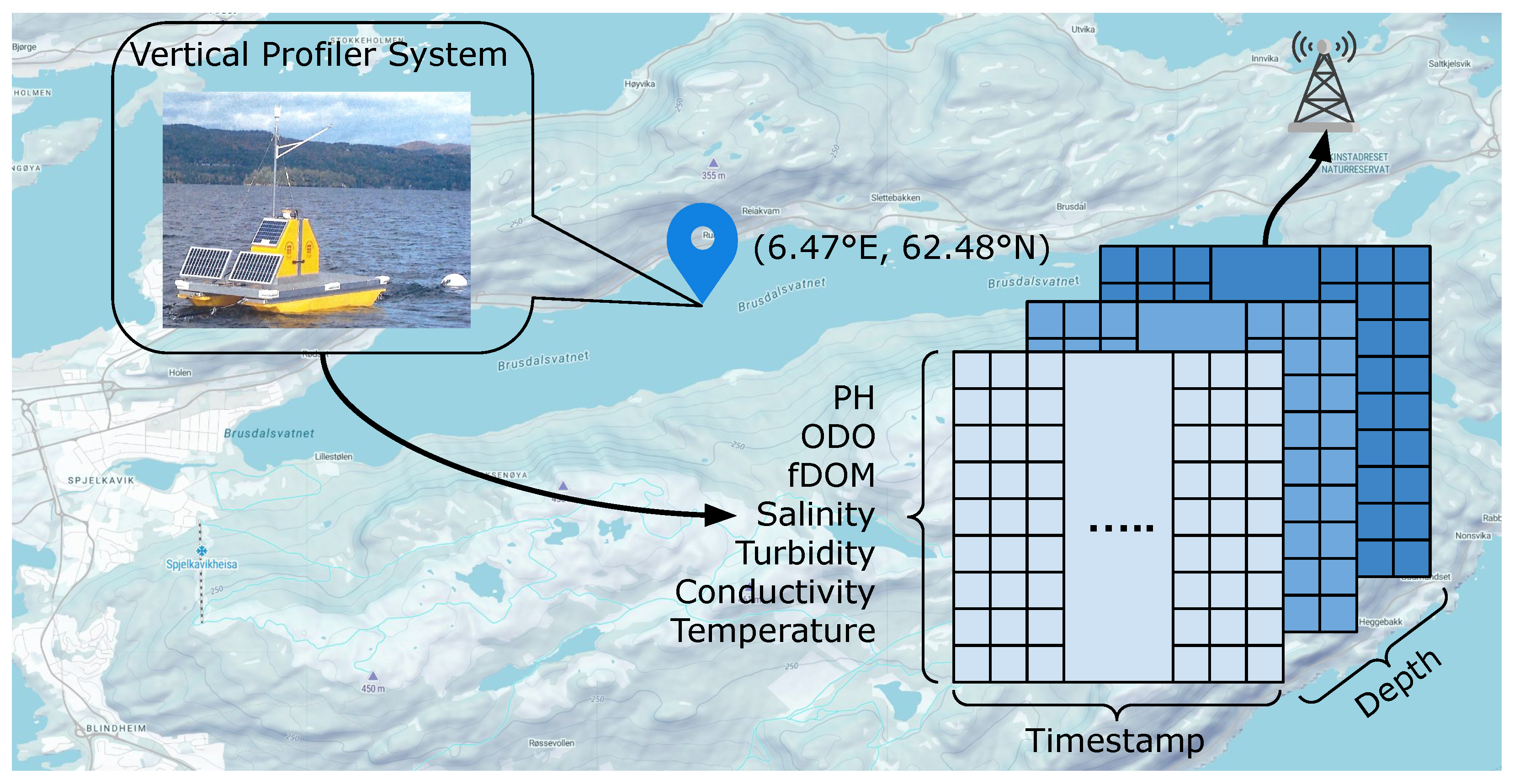
This study leverages water quality data from a Vertical Profiler System, an anchored sensor platform made by the Water and Environmental Engineering Group at NTNU in Ålesund. The sensor platform is located at 62.48° N and 6.47° E in Brusdalsvatnet Lake in Ålesund, Norway, as depicted in Figure 2. The platform has an on-board winch system with a multi-parameter sensor (EXO3) that autonomously measures water quality parameters at different depths of its profiling location. The parameters accounted for are temperature, conductivity, salinity, turbidity, pH, optical dissolved oxygen (ODO), and fluorescent dissolved organic matter (fDOM), as depicted in Figure 3. However, in this study, only pH and turbidity are being studied due to the lack of clean data for other parameters. Data on the parameters are relayed to a local server via a 900 MHz radio link. The stored data are structured as interlinked time series.
For the purposes of this study, the dataset used was from 9 June 2020 to 19 August 2022. This period covers the first phase of the platform installation, where significant anomalies in the dataset from the platform were recorded. Table 1 provides a descriptive overview of the raw data collected during the period. The count column indicates the number of observations for each parameter, while the min and max columns indicate the minimum and maximum values for each parameter. The mean column presents the average value for each parameter, and the missing data column shows the number of missing values for each parameter. However, the total amount of data is less than anticipated due to the platform’s inoperability during the lake’s freezing periods (usually from December to March) or the sensor platform’s maintenance. By examining the mean values, it is apparent that not all the data are reliable. For instance, the average pH should not be 2.60, which indicates a strong acid. Moreover, considering both the minimum and maximum values, it is apparent that the raw data contain outliers in all indicators except timestamps and depths.
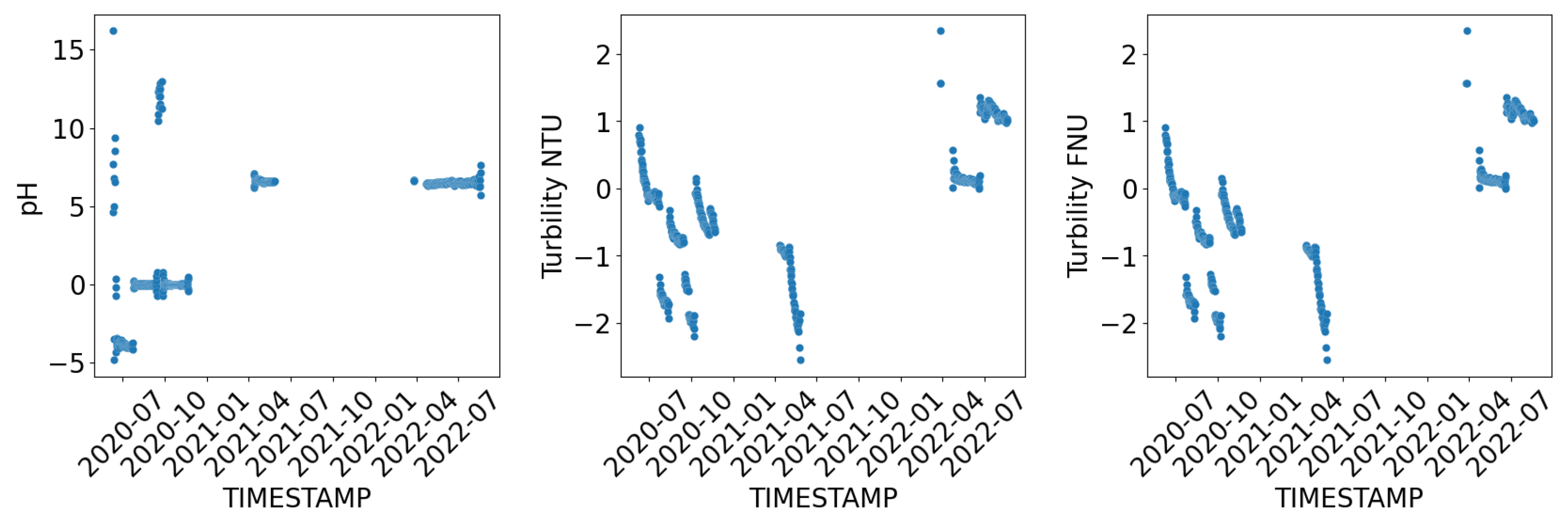
To investigate the events that occurred on the platform, Figure 4 illustrates the temporal dynamics of each sensor with a depth of 1 m. By comparing the differences between the events and the recordings, we can assume the time and provide explanations for the events. For instance, the decline in measurements on 22 November 2020 and 11 April 2021, as well as 28 May 2021 and 23 March 2022, was due to winter maintenance and broken sensors, respectively. Even minor changes, such as the sensor calibration on 26 September 2020, can impact the data’s usability and necessitate data cleaning procedures.
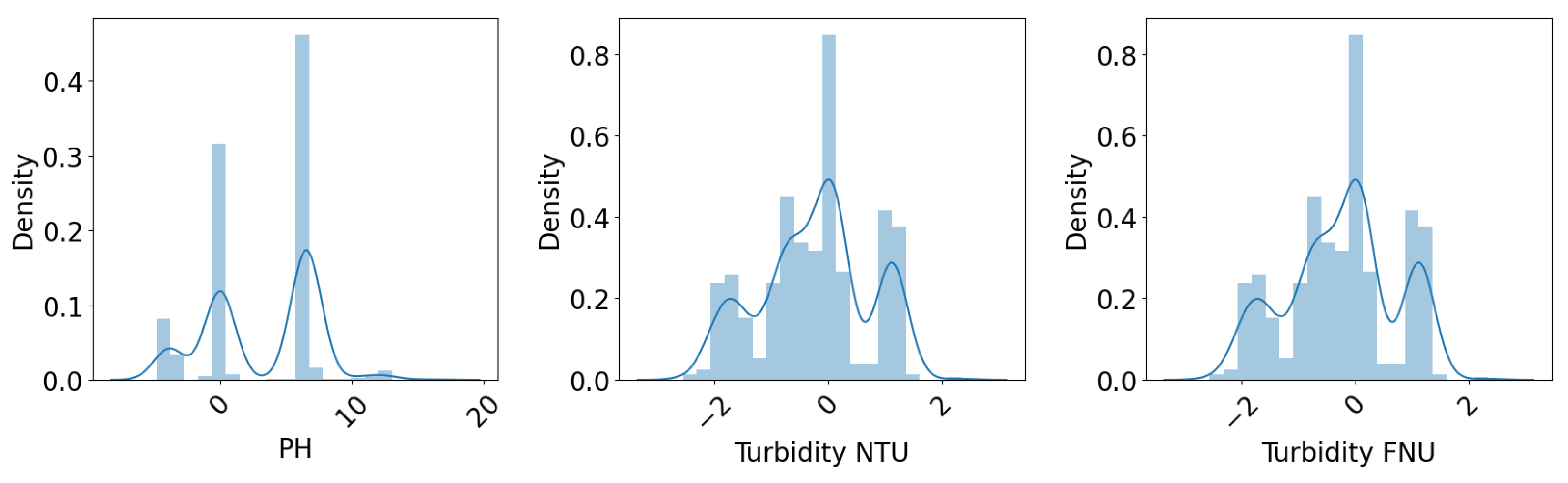
Further analysis is conducted through the data distribution, as depicted in Figure 5. It can be observed that the other sensor data do not follow normal distributions, for example, pH has three peaks while both turbidity NTU and turbidity FNU have several local maximum points as well. According to the experts, this deviation is not always incorrect. With their assistance, the sensor error label was added. The objective of the calibration was to make the sensor data as close to the clean data as possible in terms of distribution, mean value, and standard deviation.
The detection and correction of missing data are important in any data analysis project. However, in this project, only spiky data and drift data were considered for calibration. This is because the amount of missing data in the test dataset was small and the low sampling frequency of the sensor data, which was collected every 12 h, made missing data less of an issue. Therefore, the focus was primarily on correcting spiky and drift data, which have a greater impact on the accuracy and reliability of the data analysis. Four labels were attached to the test dataset, where group 0 represents no error, group 1 represents spiky data, group 2 represents drifted data, and group 3 represents both types of error.
2.2. Water Quality Anomaly Detection
The initial step after collecting raw data in this project is anomaly detection, which aims to classify the signal based on the presence of outliers and the type of fault. Figure 6 depicts the workflow. The data from various sensors are combined using a recurrence map based on location. Subsequently, a CNN is employed to classify the data into different categories based on the presence of anomalies. The effectiveness of this anomaly detection component is evaluated using training loss and accuracy and a confusion matrix.
A recurrence map, as its name suggests, is a visualization tool used to analyse the repetition of data or patterns in given sequences. It works by comparing the distance between two states of a system, and expressing the difference using the following equation [31]:
In this equation, R represents the distance, while and denote the points in the sequence. is a predefined standard number used for measuring distance. If the distance between the two states is not greater than , R is calculated as the number of differences. Otherwise, it is calculated as the maximum difference, which is defined as N. Once a signal is provided, the Euclidean distances between every pair of statuses is calculated and form the recurrency matrix, with dimensions equal to a predefined window length. With such a matrix, an image-like form of the data can be generated for further analysis.
The architecture of the CNN network is illustrated in Figure 7 and the input data are from the 2D recurrence matrix with a dimension equal to a predefined window length. With reference to the labels, the network will adjust the weights and biases in every layer according to the accuracy. By leveraging 2 convolutional and 2 pooling layers, the input matrix is transformed into feature maps. A dropout layer is then applied to avoid overfitting and flattened into a feature vector. Lastly, a fully connected layer is applied to extract the classification of the sensor data. It is a multilayer perceptron neural network. The extracted features are calculated with
where x and y are the input features and output classifications, respectively, and is the linear weights [32]. It is noted that the Softmax activation function is used for the last layer of the CNN classifier since it is a multiclass classification problem. Softmax is an activation function that is used to normalize a vector such that the sum of all the elements in the resulting vector is equal to one. It is mathematically represented in Equation (3) [33]. Here, represents the element in a vector, and C represents the dimension of the input vector.
By using this equation, the probability distribution among different classes can be calculated, and the trainable parameters can be adjusted to minimize the loss function, which is defined as categorical cross-entropy. It is calculated using Equation (4) [34], where y and are the true one-hot encoded vector and prediction probabilities for each class of the instance.
2.3. Correlated Time Series Calibration with AutoEncoder
After detecting anomalies in the sensor data, the signal calibration component is employed to correct the errors. As the data are potentially to be a correlated time series, both time dynamics and correlations can be considered in order to properly calibrate the data, and thus, an AutoEncoder-based network is proposed.
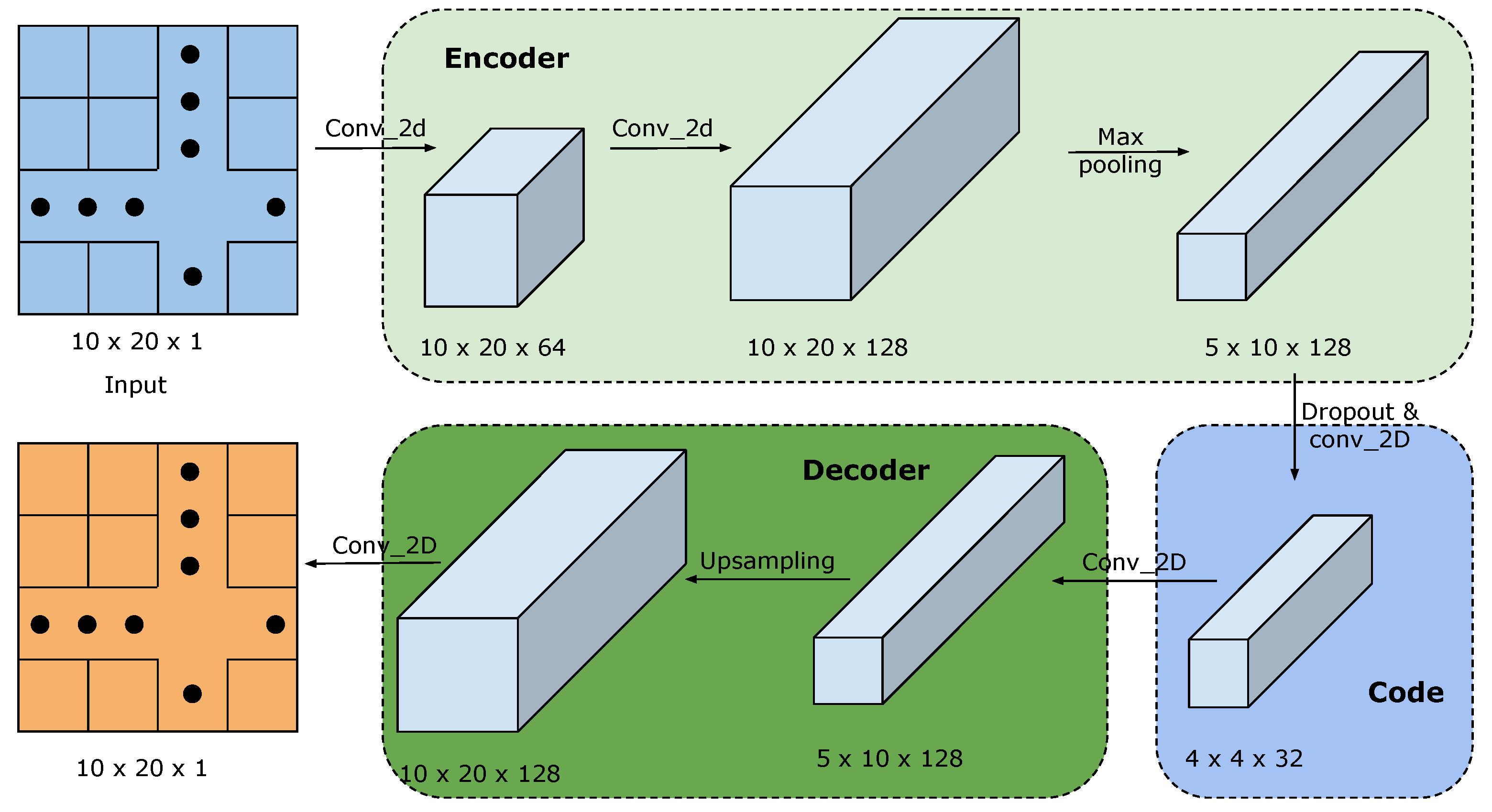
AutoEncoder is a type of neural network trained to generate an output identical to the input. Although the output and input are not exactly the same, they remain consistent with each other in probabilistic terms such as mean and standard deviation [35]. Thus, it is commonly utilized for dimensionality reduction and image denoising. The AutoEncoder model, as shown in Figure 8, can be divided into two parts: the encoder, which receives input data and processes it to generate a code; and the decoder, which regenerates the data from the code to make it as similar to the input data as possible. This process enables the AutoEncoder to extract important features from the input data and remove noise. At the beginning of this model, data are encoded into a 2D tensor, where both temporal and correlation information will be considered. The tensor is of dimensions , where 10 indicates the number of indicators considered, 20 is the length of the time series window, and 1 is the channel number. Specifically, each tensor is comprised of 20 samples containing all the measured parameters.
In an AutoEncoder network, the trainable parameters can be represented by Where and are the weight matrix and bias vector for the encoder layer, while and are the weight matrix and bias vector for the decoder layer [36]. For both encode and decode operations, the rectified linear unit (ReLU) activation function, as shown in Equation (5), was selected [37].
Thus, the element of compressed code can be expressed as [36]
where ∗ is the convolution layer operations and s is the activation function.
With the calculation result, the regenerated data can be obtained through [36]
where H is the collection of feature maps.
Unlike the traditional AutoEncoder model, which measures the difference between input and output data, the error in this project is considered as the difference between uncorrupted data and regenerated data while estimating the effectiveness of the proposed model. In this project, the sigmoid function, as shown in Equation (8) [38], was chosen to measure the cross-entropy error, and thus, minimize it during the training process.
2.4. Water Quality Clustering with Self-Organizing Map (SOM)
SOM clustering is an unsupervised machine learning algorithm. It was first proposed by Teuvo Kohonen in 1982 in [39]. Basically, it receives n-dimensional input vectors and feeds them into a neuron network to generate a two-dimensional map that can retain the original information in the input dataset. This map preserves the structural information of the data points in the dataset which, in other words, provides similar interconnecting weights to the neighbouring points. Moreover, the map itself also contains information about centroids. Every point on the map is related to the interconnecting weights and the points’ values represent the centroids. The size of the map indicates the assumed number of clusters. In this project, an SOM-based model was proposed to cluster the water quality data. The topology is depicted in Figure 9.
The present model utilizes input data derived from the high-quality data obtained in the previous section. To comply with the requirements of the sensor platform, the data are structured as a 3D tensor with the dimensions of location, sensors, and timestamp. The first step involves encoding this tensor into a 2D image, which organizes the data collected at the same time. One dimension of the image represents the depth while the other dimension comprises different sensor data. This transformation changes the problem into an image clustering task while preserving the spatial correlation among the data. Moreover, by analysing the data collected at various timestamps, the temporal changes in water quality can be investigated in detail. Then, the images are processed through the SOM network, which analyses the input data at the pixel level. The training process for SOM is outlined in Algorithm 1.
| Algorithm 1 Self-Organizing Map Algorithm |
|
The initialization of weight values is performed randomly for each input sample, and then, the weight at the best matching unit and its neighbouring weights are updated with a learning rate. The best matching unit is defined as where the distance between a sample and other weighted vectors is minimized, and thus, can be computed as shown in [39]:
where x is the sample vector and and are the best matching unit and weighted vector, respectively. The neighbouring weighted vectors at can be then calculated based on the value at time t as [40]
Here, is the learning rate which decays with time, following
and denotes the neighbouring kernel and is expressed as
where
Here, denotes the distance from the best-matching unit to the neighbouring data point rate while is the radius of the neighbouring area, which follows an exponentially decaying function.
The updating finishes when the convergence requirement or iteration number is reached. Normally, the convergence is the dissimilarity, which can be calculated as the distance between data points. This project achieves this by using the Euclidean distance, where the weighted vectors are used to approximate the centroid.
2.5. Evaluation Matrix
In this project, the key parameter that needs to be defined is the number of clusters, denoted by K. The selection of K is performed by comparing the distortion and silhouette score, which are used to evaluate the tightness cohesion and separation, respectively.
Distortion, also referred to as intra-cluster distance, is a widely employed measure for assessing the performance of clustering algorithms. It quantifies the average squared Euclidean distance between each data point and its corresponding cluster centroid. By evaluating distortion, researchers can determine the quality of clustering results and make informed decisions regarding the optimal number of clusters.
For the silhouette score, cohesion refers to the distance from a data point to its cluster’s centroid, while separation refers to the distance from this point to other clusters’ centroids. Specifically, the silhouette score measures the ratio of cohesion to separation, which is calculated using the following equation [41]:
Here, is the mean distance from the data point to all other data points in the same cluster, and is the average intra-cluster distance from the data point to all other clusters’ centroids.
The silhouette score has a range from −1 to 1, where a higher index indicates higher inter-cluster similarity and lower intra-cluster similarity. Specifically, 1, 0, and −1 denote the best, indifferent, and wrong clustering results, respectively.
However, both matrices have their own limitations. The distortion does not take the intra-cluster similarity into consideration and the silhouette score is sensitive to noise and cannot handle overlapping clusters. Therefore, the combined results of both metrics are used to determine the final number of clusters.
3. Results and Discussion
3.1. Results Analysis
3.1.1. Water Quality Sensor Data Anomaly Detection
The labelled data were transformed into recurrence maps, as depicted in Figure 1. To mitigate the influence of varying scales across different sensor data, the data were normalized using Equation (15):
where X represents the data series, and x and denote the original and normalized data. Here, and represent the mean value and standard deviation of the series, respectively.
Two different mapping strategies were employed in this study. The first strategy considered the temporal dynamics of each sensor by retaining the original data values and calculating the recurrence matrix, as described in Section 2.2. The second strategy involved the normalization of data from multiple sensors recorded at the same time.
After the matrices are generated, they are fed into the CNN classifier for testing. Not only the loss line is depicted but also the accuracy is presented to evaluate the model’s performance. The results can be seen in Figure 10. Although for both strategies, the overall accuracy increases with the training epoch and finally reaches a relatively stable stage, the accuracy from the normalized multisensor is higher than the unnormalized sole sensor. The former can reach as high as while the latter can only reach .
To provide a more detailed comparison, a confusion matrix was utilized. Table 2 shows the confusion matrix, which is calculated from the detection class for every class. The score, the harmonic mean of precision and recall, was applied to analyse this matrix; it can be expressed as follows:
where is defined as the ratio of true positive (TP) results to the sum of true positive and false positive (FP) results for class a, which measures the model’s ability to identify positive results, and is defined as the ratio of TP results to the sum of TP and false negative (FN) results for class a, which measures the ability to capture all positive examples. It should be noted that these are based on a single class in a multiclass classification problem. In this case, the F1 score was calculated for each class separately as 0.96, 0.71, 0.97, and 0.96 for “clean”, “drift”, “spiky”, and “both” classes, respectively.
3.1.2. Water Quality Sensor Data Reconstruction
A comparison between raw data and calibrated data at a depth of 1 m is depicted in Figure 11. In all three figures, red lines represent the original data, while blue lines represent the calibrated data. From Figure 11a, we can see that the raw pH sensor data suffered from both drift and spikiness. After 60 samples, the mean value decreases, and the variation starts increasing. Compared to these raw data, the calibrated data are more usable, showing less drift and fewer spikes. Figure 11b and Figure 11c show positive results for turbidity NTU and turbidity FNU, where drift is the primary challenge. The drift is reduced compared to the uncalibrated data, and the distribution is closer to the 60 clean data points.
To further analyse the data quality, a study of the calibrated data distribution is conducted, and the results are shown in Table 3 and Figure 12. Since no dramatic changes occurred during the data collection period, the sensor data should follow the same distribution. Thus, the mean value, standard deviation, and density distribution are examined. From Table 3, it can be observed that the regenerated pH data have the closest mean value and standard deviation, with offsets of 1.6% and 17.6%, respectively. The calibrated turbidity NTU and FNU also show smaller deviations from the clean data compared to the uncalibrated data. Although drift still exists, the mean value drops from 1.145 to 0.101, with a baseline of 0.126. This can be considered effective for data drift calibration. By examining the distribution in Figure 12, a similar conclusion can be drawn. It is common for the three parameters that the shapes formed by calibrated data are closer to the uncalibrated data.
It should be noted that the presented findings are consistent with the performance of the algorithms for other depths, given the same sensor platform, location, and data structure.
3.1.3. Water Quality Clustering
With these calibrated data, clustering algorithms can be applied to generate the final clustering for water quality monitoring. In addition to the originally clean data, the calibrated data are also taken into consideration. The combination is then fed into the clustering algorithm to evaluate the final results for our project.
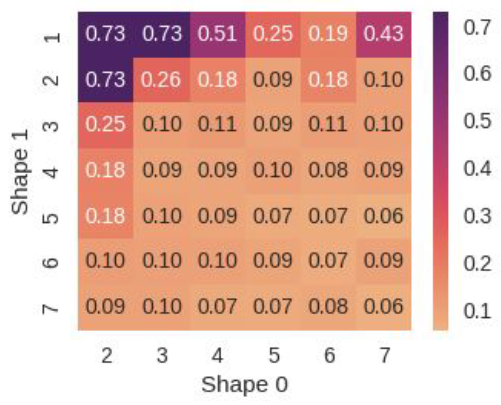
Figure 13 illustrates the outcomes obtained from applying the SOM clustering algorithm. These heatmaps enable a comparison of the silhouette scores based on different SOM grid shapes, aiding in the determination of optimal parameters. Shapes , , and exhibit identical silhouette scores of 0.73. Among these, both and indicate a tendency for samples to be clustered into two groups. However, this preference for fewer clusters stems from the silhouette score’s inclination towards selecting configurations with minimal dissimilarity within clusters and maximal dissimilarity between clusters, rather than solely considering the number of clusters. Consequently, it is crucial to consider alternative shapes that yield high scores. To this end, shape clusters the data into three distinct groups.
The clustering distribution with AutoEncoder-calibrated data is visualized in Figure 14. In this case, cluster 0 has the greatest portion of data points () while of the data are assigned to cluster 3. This indicates a balanced distribution among the clusters, which is required by the clustering algorithms.
During discussions on the clustering results, the experts emphasized the significance of determining the appropriate number of clusters. In practice, it is uncommon to have more than five clusters, especially in the context of drinking water reservoirs, where careful selection and minimal drastic changes are expected. However, merely having two clusters does not provide accurate enough results to represent the final outcome. Consequently, the experts recommended that three, four, or five clusters would be the most suitable choices. Subsequently, they examined the clustering results and confirmed that the clustering achieved using the SOM with AutoEncoder-calibrated data was reasonable and could be further explored through in-depth analysis.
3.2. Potential Limitations
The approach outlined in this project faces several limitations, specifically pertaining to environmental factors, workforce issues, and standardization challenges.
One of the primary limitations is related to the environmental conditions in which the experiments are conducted. The experimental platform is situated in a lake in Ålesund, and during the winter season, the platform freezes, rendering it incapable of collecting data. Consequently, this poses a significant obstacle in obtaining accurate and reliable data during those periods. Moreover, the surrounding environment further complicates data collection efforts. The reservoir is not located in an isolated area, as there is nearby transportation infrastructure that may introduce unwanted influences on the water quality sensors.
The second limitation revolves around the workforce involved in the project, particularly in terms of data labelling. Labelling the data is crucial not only for anomaly detection but also for enhancing calibration and clustering outcomes. Allocating additional resources to ensure the collection of accurate sensor data and establishing standardized clustering procedures would greatly improve the overall accuracy of the solution. However, acquiring access to water quality data, which is confidential, proves to be challenging, hindering the expansion of the dataset. Consequently, human labelling remains the most viable option, despite requiring a substantial labour force.
The final limitation concerns the usability of the overall solution and the need for standardization. Establishing a comprehensive set of standards is essential to enhance the system’s utility and comprehensibility. These standards would encompass indicator selection, data collection, and processing procedures, as well as the final clustering methodology. However, each city follows its own unique set of standards, and different systems are employed, further complicating the task of standardization. Overcoming this challenge presents a difficult undertaking due to the inherent variations across different locations and systems.
4. Conclusions
Currently, water source monitoring in water supply systems relies on regular sampling and analysis for microbial water quality indicators and other pollutants such as heavy metals to ensure the provision of safe drinking water to the public. However, these methods require long periods of in-laboratory processing, they are costly, and make real-time monitoring impractical. To address this limitation, a sensor platform has been implemented to collect data from Brusdalsvatnet Lake, the drinking water source for the municipality of Alesund in Norway. Yet, measurements from the sensor platform often contain anomalies, making it difficult to directly apply the data for effective management decisions. This study proposes an architecture that can enable a more rapid and efficient preprocessing and analysis of the data transmitted by the sensor platform. By implementing this proposed architecture, the water supply system can promptly identify anomalies, calibrate the data, and conduct clustering, ensuring effective management of water resources which contributes to advancements in water quality monitoring, providing valuable insights for stakeholders and decision-makers involved.
The significance of the proposed system in the water quality monitoring for the municipality was underscored by the stakeholders. They emphasized the system’s seamless data analysis capabilities, which ultimately yield substantial benefits for them by providing valuable insights into potential fluctuations in water quality. To further illustrate the potential applications of the collected data, one example is the utilization of fluid dynamics simulations. These simulations can be performed using the collected data, allowing for the prediction and assessment of water quality dynamics [42]. Moreover, the recorded data can be employed for water risk management purposes. The findings and observations derived from the monitoring system can serve as essential inputs for assessing and mitigating potential risks associated with water quality in urban water supply systems [43].
To make the whole system more feasible, the future work of this project involves expanding its scope, collecting more data, collaborating with domain experts to validate and interpret the results, and integrating the system with other relevant systems. By pursuing these avenues, we can improve the reliability, usability, and applicability of our models, enabling their effective implementation in real-life scenarios and benefiting various stakeholders involved in water quality management and decision-making processes.
Author Contributions
Conceptualization, J.L. and D.W.; methodology, J.L. and D.W.; software, J.L.; validation, J.L., D.W. and H.M.; formal analysis, J.L.; investigation, J.L.; resources, D.W. and R.S.; data curation, R.S.; writing—original draft preparation, J.L.; writing—review and editing, D.W., H.M. and R.S.; visualization, J.L.; supervision, D.W.; project administration, R.S. All authors have read and agreed to the published version of the manuscript.
Funding
This research was funded by Ålesund municipality under a smart water and wastewater infrastructure project grant number 90392200.
Data Availability Statement
The datasets presented in this article are not readily available because of the government policies in Norway. The material and code can be accessed upon reasonable request.
Conflicts of Interest
The authors declare no conflict of interest.
Abbreviations
| CNN | Convolutional neural network |
| CTS | Correlated time series |
| ReLU | Rectified linear unit |
| SOM | Self-organizing map |
| SVM | Support vector machine |
References
- Burian, S.; Walsh, T.; Kalyanapu, A.; Larsen, S. 5.06—Climate Vulnerabilities and Adaptation of Urban Water Infrastructure Systems. In Climate Vulnerability; Pielke, R.A., Ed.; Academic Press: Oxford, UK, 2013; pp. 87–107. [Google Scholar] [CrossRef]
- Price, J.I.; Heberling, M.T. The Effects of Source Water Quality on Drinking Water Treatment Costs: A Review and Synthesis of Empirical Literature. Ecol. Econ. 2018, 151, 195–209. [Google Scholar] [CrossRef] [PubMed]
- Bhateria, R.; Jain, D. Water quality assessment of lake water: A review. Sustain. Water Resour. Manag. 2016, 2, 161–173. [Google Scholar] [CrossRef]
- Lahiry, S. Impact on the environment due to industrial development in Chhattisgarh region of Madhya Pradesh. Financ. India 1996, 10, 133–136. [Google Scholar]
- Wu, D.; Wang, H.; Seidu, R. Toward A Sustainable Cyber-Physical System Architecture for Urban Water Supply System. In Proceedings of the 2020 International Conferences on Internet of Things (iThings) and IEEE Green Computing and Communications (GreenCom) and IEEE Cyber, Physical and Social Computing (CPSCom) and IEEE Smart Data (SmartData) and IEEE Congress on Cybermatics (Cybermatics), Rhodes Island, Greece, 2–6 November 2020; IEEE: Piscataway, NJ, USA, 2020; pp. 482–489. [Google Scholar]
- Banna, M.H.; Imran, S.; Francisque, A.; Najjaran, H.; Sadiq, R.; Rodriguez, M.; Hoorfar, M. Online drinking water quality monitoring: Review on available and emerging technologies. Crit. Rev. Environ. Sci. Technol. 2014, 44, 1370–1421. [Google Scholar] [CrossRef]
- Soldán, P. Improvement of online monitoring of drinking water quality for the city of Prague and the surrounding areas. Environ. Monit. Assess. 2021, 193, 758. [Google Scholar] [CrossRef] [PubMed]
- Shi, Z.; Chow, C.W.; Fabris, R.; Liu, J.; Jin, B. Alternative particle compensation techniques for online water quality monitoring using UV—Vis spectrophotometer. Chemom. Intell. Lab. Syst. 2020, 204, 104074. [Google Scholar] [CrossRef]
- Kumawat, M.; Sharma, P.; Pal, N.; James, M.M.; Verma, V.; Tiwari, R.R.; Shubham, S.; Sarma, D.K.; Kumar, M. Occurrence and seasonal disparity of emerging endocrine disrupting chemicals in a drinking water supply system and associated health risk. Sci. Rep. 2022, 12, 9252. [Google Scholar] [CrossRef] [PubMed]
- Carminati, M.; Turolla, A.; Mezzera, L.; Di Mauro, M.; Tizzoni, M.; Pani, G.; Zanetto, F.; Foschi, J.; Antonelli, M. A self-powered wireless water quality sensing network enabling smart monitoring of biological and chemical stability in supply systems. Sensors 2020, 20, 1125. [Google Scholar] [CrossRef]
- Hussain, M.; Jamir, L.; Singh, M.R. Assessment of physico-chemical parameters and trace heavy metal elements from different sources of water in and around institutional campus of Lumami, Nagaland University, India. Appl. Water Sci. 2021, 11, 76. [Google Scholar] [CrossRef]
- Custodio, M.; Peñaloza, R. Data on the spatial and temporal variability of physical-chemical water quality indicators of the Cunas River, Peru. Chem. Data Collect. 2021, 33, 100672. [Google Scholar] [CrossRef]
- Hawari, H.F.b.; Mokhtar, M.N.S.b.; Sarang, S. Development of Real-Time Internet of Things (IoT) Based Water Quality Monitoring System. In Proceedings of the International Conference on Artificial Intelligence for Smart Community, Perak, Malaysia, 17–18 December 2022; Springer: Berlin/Heidelberg, Germany, 2022; pp. 443–454. [Google Scholar]
- Fascista, A. Toward integrated large-scale environmental monitoring using WSN/UAV/Crowdsensing: A review of applications, signal processing, and future perspectives. Sensors 2022, 22, 1824. [Google Scholar] [CrossRef]
- Mohammed, H.; Longva, A.; Seidu, R. Impact of climate forecasts on the microbial quality of a drinking water source in Norway using hydrodynamic modeling. Water 2019, 11, 527. [Google Scholar] [CrossRef]
- Simitha, K.M.; Raj, S. IoT and WSN Based Water Quality Monitoring System. In Proceedings of the 2019 3rd International Conference on Electronics, Communication and Aerospace Technology (ICECA), Coimbatore, India, 12–14 June 2019; pp. 205–210. [Google Scholar] [CrossRef]
- Chen, Y.; Han, D. Water quality monitoring in smart city: A pilot project. Autom. Constr. 2018, 89, 307–316. [Google Scholar] [CrossRef]
- Munir, M.; Siddiqui, S.A.; Dengel, A.; Ahmed, S. DeepAnT: A deep learning approach for unsupervised anomaly detection in time series. IEEE Access 2018, 7, 1991–2005. [Google Scholar] [CrossRef]
- Zhang, C.; Song, D.; Chen, Y.; Feng, X.; Lumezanu, C.; Cheng, W.; Ni, J.; Zong, B.; Chen, H.; Chawla, N.V. A deep neural network for unsupervised anomaly detection and diagnosis in multivariate time series data. In Proceedings of the AAAI Conference on Artificial Intelligence, Honolulu, HI, USA, 27 January–1 February 2019; Volume 33, pp. 1409–1416. [Google Scholar]
- Muriira, L.M.; Zhao, Z.; Min, G. Exploiting linear support vector machine for correlation-based high dimensional data classification in wireless sensor networks. Sensors 2018, 18, 2840. [Google Scholar] [CrossRef] [PubMed]
- Borghesi, A.; Bartolini, A.; Lombardi, M.; Milano, M.; Benini, L. Anomaly detection using autoencoders in high performance computing systems. In Proceedings of the AAAI Conference on Artificial Intelligence, Honolulu, HI, USA, 27 January–1 February 2019; pp. 9428–9433. [Google Scholar]
- Canizo, M.; Triguero, I.; Conde, A.; Onieva, E. Multi-head CNN–RNN for multi-time series anomaly detection: An industrial case study. Neurocomputing 2019, 363, 246–260. [Google Scholar] [CrossRef]
- Guo, H.; Huang, J.J.; Chen, B.; Guo, X.; Singh, V.P. A machine learning-based strategy for estimating non-optically active water quality parameters using Sentinel-2 imagery. Int. J. Remote Sens. 2021, 42, 1841–1866. [Google Scholar] [CrossRef]
- Bao, S.; Zhang, R.; Wang, H.; Yan, H.; Chen, J.; Wang, Y. Correction of satellite sea surface salinity products using ensemble learning method. IEEE Access 2021, 11, 17870–17881. [Google Scholar] [CrossRef]
- Tenjo, C.; Ruiz-Verdú, A.; Van Wittenberghe, S.; Delegido, J.; Moreno, J. A new algorithm for the retrieval of sun induced chlorophyll fluorescence of water bodies exploiting the detailed spectral shape of water-leaving radiance. Remote Sens. 2021, 13, 329. [Google Scholar] [CrossRef]
- Maier, P.M.; Keller, S.; Hinz, S. Deep learning with WASI simulation data for estimating chlorophyll a concentration of inland water bodies. Remote Sens. 2021, 13, 718. [Google Scholar] [CrossRef]
- Arnault, S.; Thiria, S.; Crépon, M.; Kaly, F. A tropical Atlantic dynamics analysis by combining machine learning and satellite data. Adv. Space Res. 2021, 68, 467–486. [Google Scholar] [CrossRef]
- Wang, X.; Fu, L.; He, C. Applying support vector regression to water quality modelling by remote sensing data. Int. J. Remote Sens. 2011, 32, 8615–8627. [Google Scholar] [CrossRef]
- Yu, J.; Tian, Y.; Wang, X.; Zheng, C. Using machine learning to reveal spatiotemporal complexity and driving forces of water quality changes in Hong Kong marine water. J. Hydrol. 2021, 603, 126841. [Google Scholar] [CrossRef]
- Çinar, Ö.; Merdun, H. Application of an unsupervised artificial neural network technique to multivariant surface water quality data. Ecol. Res. 2009, 24, 163–173. [Google Scholar] [CrossRef]
- Eckmann, J.P.; Kamphorst, S.O.; Ruelle, D. Recurrence plots of dynamical systems. In Turbulence, Strange Attractors and Chaos; World Scientific Series on Nonlinear Science Series A; Word Scientific Publishing: Singapore, 1995; Volume 16, pp. 441–446. [Google Scholar]
- LeCun, Y. LeNet-5, Convolutional Neural Networks. 2015, Volume 20, p. 14. Available online: http://yann.lecun.com/exdb/lenet (accessed on 15 March 2024).
- Goodfellow, I.; Bengio, Y.; Courville, A. Deep Learning; MIT Press: Cambridge, MA, USA, 2016; pp. 180–184. [Google Scholar]
- Good, I.J. Rational decisions. J. R. Stat. Soc. Ser. B 1952, 14, 107–114. [Google Scholar] [CrossRef]
- Vincent, P.; Larochelle, H.; Lajoie, I.; Bengio, Y.; Manzagol, P.A.; Bottou, L. Stacked denoising autoencoders: Learning useful representations in a deep network with a local denoising criterion. J. Mach. Learn. Res. 2010, 11, 3371–3408. [Google Scholar]
- Ballard, D.H. Modular learning in neural networks. In Proceedings of the 6th National Conference on Artificial Intelligence, Seattle, WA, USA, 13–17 July 1987; Volume 1, pp. 279–284. [Google Scholar]
- Hara, K.; Saito, D.; Shouno, H. Analysis of function of rectified linear unit used in deep learning. In Proceedings of the 2015 International Joint Conference on Neural Networks (IJCNN), Killarney, Ireland, 12–17 July 2015; IEEE: Piscataway, NJ, USA, 2015; pp. 1–8. [Google Scholar]
- Han, J.; Moraga, C. The influence of the sigmoid function parameters on the speed of backpropagation learning. In Proceedings of the International Workshop on Artificial Neural Networks, Perth, WA, Australia, 27 November–1 December 1995; Springer: Berlin/Heidelberg, Germany, 1995; pp. 195–201. [Google Scholar]
- Kohonen, T. Self-Organization and Associative Memory; Springer Science & Business Media: Berlin/Heidelberg, Germany, 2012; Volume 8. [Google Scholar]
- Kohonen, T. The self-organizing map. Proc. IEEE 1990, 78, 1464–1480. [Google Scholar] [CrossRef]
- Rousseeuw, P.J. Silhouettes: A graphical aid to the interpretation and validation of cluster analysis. J. Comput. Appl. Math. 1987, 20, 53–65. [Google Scholar] [CrossRef]
- Neba, F.A.; Asiedu, N.Y.; Addo, A.; Morken, J.; Østerhus, S.W.; Seidu, R. Simulation of two-dimensional attainable regions and its application to model digester structures for maximum stability of anaerobic treatment process. Water Res. 2019, 163, 114891. [Google Scholar] [CrossRef]
- Wu, D.; Seidu, R.; Wang, H.; Ban, X. A Case-Based Reasoning Solution for Urban Drinking Water Quality Control. In Proceedings of the 2021 IEEE 23rd Int Conf on High Performance Computing & Communications; 7th Int Conf on Data Science & Systems; 19th Int Conf on Smart City; 7th Int Conf on Dependability in Sensor, Cloud & Big Data Systems & Application (HPCC/DSS/SmartCity/DependSys), Haikou, China, 20–22 December 2021; IEEE: Piscataway, NJ, USA, 2021; pp. 2454–2459. [Google Scholar]
Figure 1.
System overview of the whole project.

Figure 2.
Location of the water reservoir being studied.

Figure 3.
Information about the sensor platform.

Figure 4.
Time series visualization of sensor data.

Figure 5.
Distribution of flattened sensor data.

Figure 6.
Processing for anomaly detection.

Figure 7.
CNN network structure.

Figure 8.
AutoEncoder structure overview.

Figure 9.
Topology of self-organizing map.

Figure 10.
The training loss and accuracy change with epoch.

Figure 11.
Comparison of calibration results to original data.

Figure 12.
Density distribution comparison of clean data, uncalibrated data, and AutoEncoder-calibrated data.
Figure 12.
Density distribution comparison of clean data, uncalibrated data, and AutoEncoder-calibrated data.

Figure 13.
Silhouette score heatmap for shape analysis with AutoEncoder-calibrated data.

Figure 14.
Clustering distribution with SOM using AutoEncoder-calibrated data.


Table 1.
Description of the raw dataset.
| Parameter | Count | Min | Max | Mean | Missing Data |
|---|---|---|---|---|---|
| Timestamp | 38,675 | 9 June 2020 15:14:06 | 19 August 2022 01:18:29 | / | 0 |
| Depth | 38,765 | 1 | 81 | 32.86 | 0 |
| pH | 38,765 | −4.35 | 141.87 | 2.60 | 0 |
| Turbidity NTU | 38,765 | −2.24 | 36.92 | −0.25 | 0 |
| Turbidity FNU | 38,765 | 0.836 | 81.036 | 32.86 | 0 |
Table 2.
Confusion matrix for anomaly classification.
| Total Samples = 11,335 | Prediction (%) | ||||
|---|---|---|---|---|---|
| Clean | Drift | Spiky | Both | ||
| Ground truth | Clean | 2370 | 85 | 68 | 0 |
| Drift | 7 | 3381 | 0 | 99 | |
| Spiky | 56 | 0 | 2290 | 0 | |
| Both | 0 | 120 | 0 | 2859 | |
Table 3.
Distribution comparison among clean data and calibrated data.
| Source | pH | Turbidity NTU | Turbidity FNU | |||
|---|---|---|---|---|---|---|
| Mean | Std | Mean | Std | Mean | Std | |
| Clean data | 6.36 | 0.034 | 0.12 | 0.018 | 0.13 | 0.012 |
| Uncalibrated data | 6.38 | 0.11 | 1.15 | 0.054 | 1.14 | 0.52 |
| Calibrated data | 6.35 | 0.040 | 0.10 | 0.017 | 0.10 | 0.017 |
Disclaimer/Publisher’s Note: The statements, opinions and data contained in all publications are solely those of the individual author(s) and contributor(s) and not of MDPI and/or the editor(s). MDPI and/or the editor(s) disclaim responsibility for any injury to people or property resulting from any ideas, methods, instructions or products referred to in the content. |
© 2024 by the authors. Licensee MDPI, Basel, Switzerland. This article is an open access article distributed under the terms and conditions of the Creative Commons Attribution (CC BY) license (https://creativecommons.org/licenses/by/4.0/).
Share and Cite
MDPI and ACS Style
Liu, J.; Wu, D.; Mohammed, H.; Seidu, R. A Novel Method for Anomaly Detection and Signal Calibration in Water Quality Monitoring of an Urban Water Supply System. Water 2024, 16, 1238. https://0-doi-org.brum.beds.ac.uk/10.3390/w16091238
AMA Style
Liu J, Wu D, Mohammed H, Seidu R. A Novel Method for Anomaly Detection and Signal Calibration in Water Quality Monitoring of an Urban Water Supply System. Water. 2024; 16(9):1238. https://0-doi-org.brum.beds.ac.uk/10.3390/w16091238
Chicago/Turabian StyleLiu, Jincheng, Di Wu, Hadi Mohammed, and Razak Seidu. 2024. "A Novel Method for Anomaly Detection and Signal Calibration in Water Quality Monitoring of an Urban Water Supply System" Water 16, no. 9: 1238. https://0-doi-org.brum.beds.ac.uk/10.3390/w16091238
Note that from the first issue of 2016, this journal uses article numbers instead of page numbers. See further details here.