Article

Identification of Trends in Dam Monitoring Data Series Based on Machine Learning and Individual Conditional Expectation Curves

by
Miguel Á. Fernández-Centeno
1,2,*,
Patricia Alocén
1,2 and
Miguel Á. Toledo
1
1
ETS de Ingenieros de Caminos, Canales y Puertos, Universidad Politécnica de Madrid (UPM), Profesor Aranguren s/n, 28040 Madrid, Spain
2
ACIS Innovation+Engineering S.L. (ACIS2in), Lucio Muñoz 4, 28982 Parla, Spain
*
Author to whom correspondence should be addressed.
Submission received: 22 March 2024 / Revised: 22 April 2024 / Accepted: 25 April 2024 / Published: 26 April 2024

Abstract

:
Dams are complex systems that involve both the structure itself and its foundation. Rheological phenomena, expansive reactions, or alterations in the geotechnical parameters of the foundation, among others, result in non-reversible and cumulative modifications in the dam response, leading to trends in the monitoring data series. The accurate identification and definition of these trends to study their evolution are key aspects of dam safety. This manuscript proposes a methodology to identify trends in dam behavioural data series by identifying the influence of the time variable on the predictions provided by the ML models. Initially, ICE curves and SHAP values are employed to extract temporal dependence, and the ICE curves are found to be more precise and efficient in terms of computational cost. The temporal dependencies found are adjusted using a GWO algorithm to different function characteristics of irreversible processes in dams. The function that provides the best fit is selected as the most plausible. The results obtained allow us to conclude that the proposed methodology is capable of obtaining estimates of the most common trends that affect movements in concrete dams with greater precision than the statistical models most commonly used to predict the behaviour of these types of variables. These results are promising for its general application to other types of dam monitoring data series, given the versatility demonstrated for the unsupervised identification of temporal dependencies.

1. Introduction and Background

Dams, like any other infrastructure, respond to external and internal loads. The anisotropy and evolution of the mechanical properties of the materials they are composed of and their foundations make the whole system complex and evolutionary.
The mechanical response of the dam to variations in external variables exhibits reversible behaviour as long as the materials remain in the elastic zone. However, plasticization of materials, rheological changes, expansive chemical reactions, or degradation due to external factors impose irreversible deformations. Identification and definition of these trends are key to dam safety.
Traditional tools for trend detection in time series, such as dam monitoring data, are based on univariate analysis. A large number of scientific references on this topic can be found applied to various fields [1,2,3].
These methods, as univariate, do not consider possible trends in loads as the temperature increases or the water levels decrease due to global climate change. Therefore, the trends of the behavioural variables of a dam defined by such univariate models may be influenced by the trends that the causal variables may exhibit and, consequently, may not adequately reflect the irreversible variations in its structural response mode, leading to a misinterpretation of the structural health of the dam.
Therefore, it is necessary to identify irreversible variations in the dam response (trends) using models that consider both behavioural variables and loads.
The most common models that relate causal and behavioural variables in current practice for dam safety monitoring are statistical models such as HST, HTT, variants thereof, or other types of multiple linear regression [4,5].
Numerical models, because of the significant heterogeneity of materials and complexity of the physical processes governing the dam’s response to external solicitations, as well as their high computational cost, are less widely used in monitoring instrumentation data.
The use of artificial intelligence (AI) models applied to dam safety has proliferated in recent times. Numerous scientific references related to the use of ML, DL, or hybrid models with other types of models such as statistical, time series, or physics-based numerical models can be found [6,7,8,9,10,11,12]. Machine Learning models have shown good performance in monitoring data prediction and are more accessible to interpretation than DL models. However, despite the fact that these types of models generally provide better accuracy in predictions than any of the former, the practical application of such models is currently far from commonplace. This may be due to their label as black-box models.
For the consideration of irreversible effects attributable solely to the time variable, statistical models incorporate a series of terms that depend exclusively on this variable. The response part corresponding to these terms is then interpreted as the trend in the behaviour of the target variable. If the actual trend does not correspond to the shape of the function incorporated in the regression through the terms dependent on the time variable, the irreversible behaviour obtained with the model will lead to a misinterpretation of the structural response, not only because it cannot adjust to the actual trend, but also because it affects the coefficients of the other terms during least squares fitting.
Behaviour models based on Machine Learning do not impose any predetermined form of relationship between variables on the model and can incorporate time as just another feature among the dataset with which they are trained. In this way, data-driven models based on Machine Learning can learn, during their training stage and from monitoring data, how the dam’s response changes over time while considering the rest of the causal variables at the same time.
In these black-box models, the interpretation of the relationships between different variables and the target variable is not direct, as it is in statistical models, and requires specific methods. In the literature, multiple references can be found on the interpretation or explanation of these types of complex models.
Cortez et al. [13], proposed different Sensitivity Analysis (SA) methods mainly focused on determining the importance of the inputs. He suggested the use of a Variable Effect Characteristic (VEC) curve to visualise the average impact of a given input in the model response based on the mean or median values of the rest of the inputs.
Based on this work, Lin et al. [14] proposed a method for explanation of an Optimized Sparse Bayesian Learning. The explanation was focused on the relative importance of the input variables.
Lundberg et al. [15] presented the Shapley Additive Explanations (SHAP) method to interpret predictions in complex models. Based on additive feature attribution methods and game theory, SHAP values provide the expected change in model prediction when a particular feature is conditioned.
Shao et al. [16] used SHAP methods to evaluate the importance of factors involved in a multiple monitoring point (MMP) model orientated to predict settlements in a CFRD dam and to gain control of the settlement trends in this type of dam.
Tursunalieva et al. (2024) [17] conducted a review of techniques for interpreting ML models, fundamentally classifying them into different categories: model-based, representation-based, and post hoc models. Within this latter group, they include methods such as the aforementioned SHAP, the Local Interpretable Model-Agnostic Explanations (LIME) introduced by Ribeiro et al. (2016) [18], or the GradCAM focused on Deep Learning models proposed by Selvaraju et al. (2019) [19], as model explanation techniques that allow understanding the logic behind complex ML models.
Individual Conditional Expectation curves (ICE), introduced by Goldstein (2015) [20], are a visual tool used in the analysis of regression models to understand the relationship between a specific predictor variable and the response variable. These curves show how the conditional expectation of the target variable changes for a specific record, as the explanatory variable under analysis varies while keeping the other variables constant. In other words, they provide a graphical representation of the relationship between an independent variable and the response at an individual level.
The use of ICE curves has become popular in the context of Machine Learning model interpretability [21,22] and enables the acquisition of a detailed perspective on how a particular variable influences the predictions of the model.
Appley (2020) [23] warns about the use of this type of analysis in data sets with strongly correlated variables due to the possibility of considering unlikely combinations of these variables in the calculation of partial dependence and proposes the alternative Accumulated Local Effects plots (ALE plots). Baucells (2021) [24] compared ICE and PDP with other alternatives, including ALE plots, preferring the former.
The use of ICE curves or PDP in dam safety to interpret the relations found by ML models between target variables and regressors, including time as a trend indicator, has been proposed by authors [25,26,27,28]. These authors interpret the temporal dependence obtained by these methods as the part of the behaviour that is related only to time or the existing trend. However, since the real trend is not known, the validity of this interpretation cannot be evaluated.
More complex and difficult to explain Deep Learning models can also be used for predicting the behaviour of dams. Several authors have included interpretability within the main objectives of their research [29]. In these cases, the explanation has also been aimed at determining the importance of the inputs in the predictions provided by the models.
Given the expressed need to understand and evaluate dam behaviour in terms of their safety, particularly those behaviours that do not constitute a response to the measured causal variables and result in irreversible behaviours, the objective of this research is to define an effective methodology capable of identifying and properly defining trends in dam behaviour. To achieve this, the following actions are necessary:
  • Determine whether the partial dependency or conditional expectation obtained by methods of interpreting complex ML models is representative of the actual trend existing in dam behaviour.
  • Evaluate whether these dependencies respond as expected from an engineering perspective, and if not, define a method to rationalise the results obtained from this perspective.
  • Compare the results with those that would be obtained from a conventional statistical model, such as multiple linear regression commonly used today to monitor the evaluation of this type of dam [30,31].

2. Overview of the Methodology

Although data on dam behaviour showing irreversible movements are available, trends are not known a priori, making it impossible to verify the goodness of identification carried out by ML models.
Therefore, to evaluate the ability of ML models to identify the irreversible part of movement behaviour, it is necessary to have data sets that incorporate known trends. Given the complexity of the processes behind dam monitoring data, the problem is addressed in two phases of increasing complexity.
In the first phase, the generic capacity of ML methods to identify trends coupled with pure periodic synthetic series is evaluated. A set of synthetic cases is created by adding different trend laws to a pure periodic carrier series. Predictive models of these series are developed using various ML methodologies. The part of the model response corresponding to the time variable is extracted through a conditional expectation method and compared with the trend introduced in the series. The analysis of the results obtained provides information on the theoretical capacity of the ML models and interpretation methods to identify the trend.
In the second phase, the complexity inherent in dam monitoring data series is introduced. To obtain a series similar to that corresponding to real behaviour in which the real trend is known in advance, the same trend laws applied in the previous phase are introduced into a set of real data that do not show temporal dependence or irreversible behaviours. Since it is not known a priori if the data obtained from the monitoring of a real dam exhibit any trend, an HTT model is developed on a series of real movements in the pendulum of an arch dam. When time-dependent polynomial terms are removed from the HTT model, the resulting series is taken as a stationary behaviour series (without trend). Different trend laws are added to these series to proceed in the same way as with the pure synthetic cases.
The workflow for both phases of the study would proceed as follows.
  • Creation of synthetic stationary data series: pure oscillatory functions in Phase I and stationary series based on real dam behaviour data in Phase II;
  • Selection of trend shape functions and creation of trend series;
  • Generation of experiments: synthetic data series with a trend developed by combining the two above;
  • Development of prediction models for the series: neural networks (NN), Support Vector Machines (SVM), Boosted Regression Trees (BRT), and HTT models;
  • Extraction of the response part associated with the time variable using both ICE curves and SHAP values, methods for interpretation of ML models in three tests, measurement and comparisons of results, selection of the interpretation method to use, and application to all the experiments of the phase;
  • Fitting functions to the different extracted trends through regression;
  • Determination of the error obtained on the real irreversible components.
The work concludes with an analysis and discussion of the results obtained.
In Figure 1, a general outline of the methodology followed is provided.

3. Methodology

This section outlines the approaches taken for the development of each of the tasks that make up the methodology followed.

3.1. Generation of Stationary Series

As indicated, to evaluate the trend identification capability of the different ML methods analysed, it is necessary to have series where the trend is known. To achieve this, the approach is to create stationary series to which the irreversible term of the predefined trend is added, thus creating time series with known trends.
Two types of synthetic stationary series were proposed:
  • Pure synthetic stationary series: stationary oscillatory series with constant frequency.
  • Behaviour-based stationary series: series based on real behaviours of stationary dams.

3.1.1. Pure Synthetic Stationary Series

To create a stationary oscillatory synthetic series, hereafter referred to as a pure synthetic series, a dataset of n real data points was taken from monitoring the radial movement of a direct pendulum in an arch dam. For this movement, a multiple linear regression model of the type HTT was trained, producing the coefficients of the corresponding polynomial.
z i = a 0 + a 1 h i + a 2 h i 2 + a 3 h i 3 + a 4 h i 4 + a 5 h i 5 + a 6 T a i r , i + a 7 T a i r _ m m 15 ,   i + a 8 T a i r _ m m 30 ,   i + a 9 T a i r _ m m 60 ,   i + a 10 T a i r _ m m 90 ,   i + a 11 T i + a 12 e T i   i 1 : n
where
z i is the radial movement of the pendulum at register i;
a k is the coefficient of term k in the polynomial;
h i is the water level at register i;
T a i r ,   i is the air temperature at register i;
T a i r _ m m d d ,   i is the moving average of the last dd registers of the air temperature at register i;
T i is the temporal index of register i.
Two sinusoidal oscillatory series ( x i j ) ,   j 1,2 ,   i 1 : n   were generated within the ranges covered by the water level (j = 1) and temperature (j = 2) variables of the dam dataset ( y i j ) using the following expression:
x i , j = sin 2 π T i 365 y m a x , j y m i n , j + y m e d , j
Using these series, a synthetic stationary oscillatory series was constructed employing the same regression polynomial trained on the monitoring data:
z ~ i = a 0 + a 1 x i , 1 + a 2 x i , 1 2 + a 3 x i , 1 3 + a 4 x i , 1 4 + a 5 x i , 1 5 + a 6 x i , 2 + a 7 x i , 2 _ m m 15 + a 8 x i , 2 _ m m 30 + a 9 x i , 2 _ m m 60 + a 10 x i , 2 _ m m 90 + a 11 T i + a 12 e T i   i 1 : n
where
z ~ i is the synthetic oscillatory variable at register i;
x i , 2 _ m m d d is the moving average at register i of x i , 2   over the last dd registers.
The pure synthetic stationary series obtained show the data Statistics and appearance as shown in Table 1 and Figure 2 below:

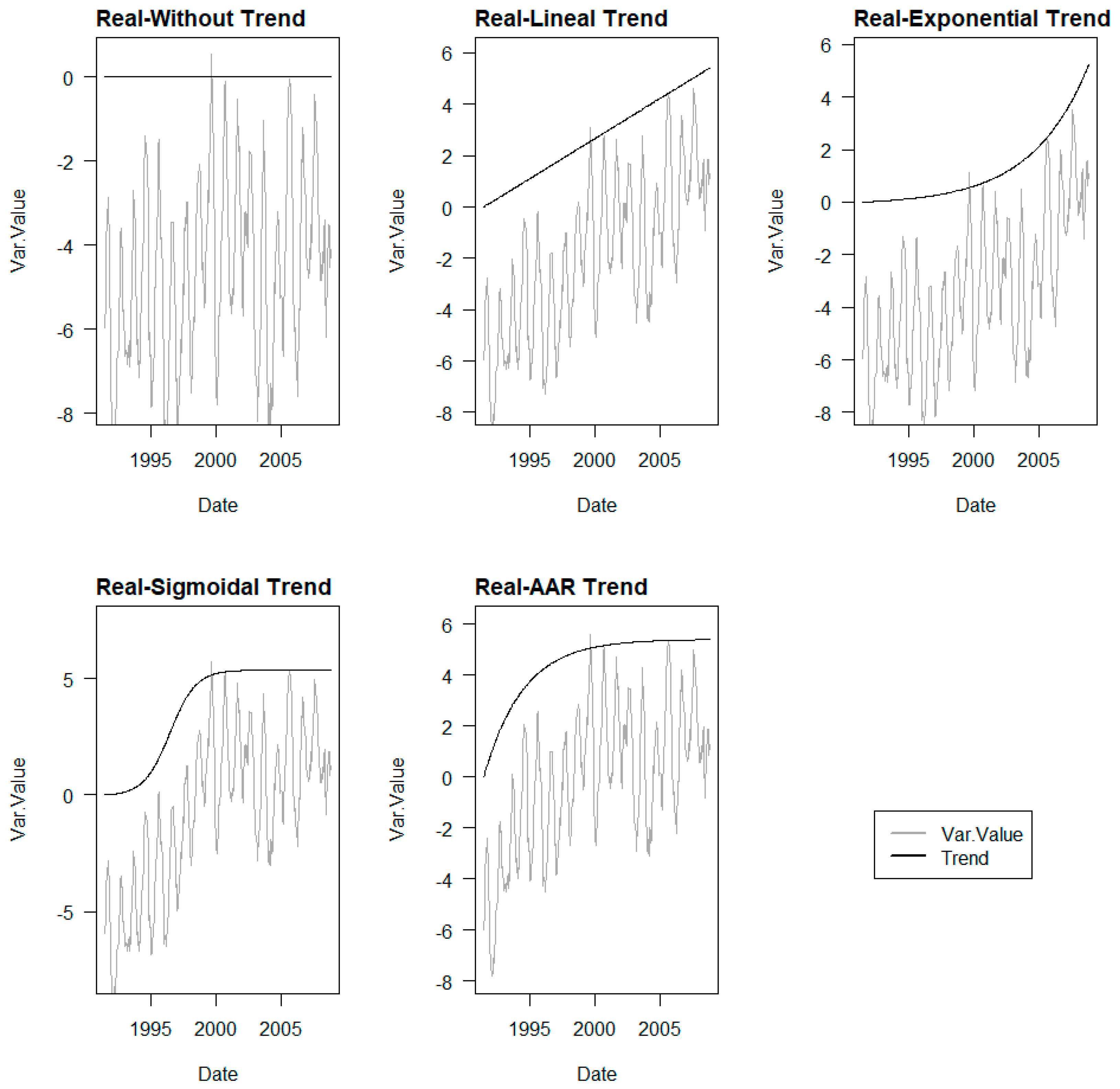
3.1.2. Behaviour-Based Stationary Series

The behaviour of monitored variables in dams, while exhibiting seasonal components and oscillatory characteristics, deviates from pure synthetic stationary series as it responds to a much more complex system. Therefore, the development of synthetic series that, while stationary, captures this behaviour is proposed in order to assess the ability of ML models to identify trends.
To obtain this kind of series, we started with the HTT model trained on a data set of n real data points from the radial movement of a direct pendulum in an arch dam, using the same expression as used to create the pure synthetic series.
This HTT model incorporates two time-dependent terms + a 11 T i + a 12 e T i . By setting the calibrated polynomial coefficients a11 and a12 to zero, the series of predicted movement without considering the temporal effect will be obtained.
The behaviour-based stationary series obtained show the data Statistics and appearance as shown in Table 2 and Figure 3 below:

3.2. Generation of Trend Series

With the aim of evaluating the generality of the methodology, the use of different trend laws was proposed: linear, exponential, sigmoidal, and expansive reaction in concrete. These types of law are the most common in the movements recorded in dams. Depending on the process that governs these drifts and their degree of development, different types of trends can be encountered.
Geotechnical instability of the foundation can lead to linear creep phenomena over very long periods of time or to faster collapse phenomena in which the deformation rate increases exponentially over time. Other processes, such as expansive reactions in concrete, exhibit a slow onset in their development, which increases until a maximum expansion rate is reached and then gradually decreases until they practically stop. Thus, they respond to sigmoidal functions. Depending on the start point of the dam movement records, the data period, and the reactivity of the process, observations will generally cover a portion of these functions. Two sigmoidal formulations are used: a generic formulation in which the complete form of the function is developed, and another, proposed by Araujo (2005) [32] for the characterisation of residual movements observed on the crest of dams affected by internal reactions, which is introduced only for decreasing slope ranges.
Consequently, the corresponding series of n records was constructed according to the following formulations:
  • Linear Trend: t l , i = m · T i + k l , where Ti is the time variable, m is the slope of the line, and kl is the y-intercept.
  • Exponential Trend: t e , i = d · p T i + k e , where Ti is the time variable, d is the amplification parameter, p is the parameter associated with the growth rate of the trend, and ke is the y-intercept.
  • Sigmoidal Trend: t s , i = q · 1 1 + e T i k 1 k 2 k s , where Ti is the time variable, q is the parameter controlling the total increment in the y-axis, k1 is the parameter defining the time position of the inflection point of the function, k2 is the parameter defining the slope at the inflection point, and ks is the y-intercept at time zero.
  • Expansive Reaction Trend: t r , i = k a + B 1 e T i C p , where Ti is the time variable, ka is the value of the y-intercept, B is the value of the y-intercept corresponding to the maximum increment, C is the time of the inflection point, and p is the parameter influencing the shape of the curve.

3.3. Generation of Experiments

Using the defined stationary series and trends, a battery of experiments is generated by their combination to evaluate the ability of ML models to identify trends in the series.
Thus, the experiments are divided into two main groups to be developed in Phase I and Phase II, based on the pure synthetic series and the stationary behaviour series, respectively.
Each type of base series is combined with the different trends, resulting in four series in each phase, to which the base series without trend of each type is added. In total, five series compose each of the two phases.

3.4. Development of Prediction Models

For each series, four types of prediction model are trained: SVM, BRT, NN, and HTT, resulting in a total of 20 experiments per phase, 40 experiments in total.
To avoid overfitting of the models during calibration, the cross-validation (CV) method was used. With this method, the training data set is divided into a series of n folds and n models are trained, each using one of the folds for training and the remaining fold for validation.
The division of the folds can be performed randomly or by sequential blocks. In this case, the latter strategy was employed, which is more suitable for modelling the behaviour of dams because, in time series where various regressors are involved, random division may provide the model with information from neighbouring records that could influence its interpretation.
Thus, in this research, one fold was taken for each year of data in the series.
To select the hyperparameters of each model, a brute-force algorithm or a grid search was employed.
The hyperparameters tuned by grid-search in each ML model were the following:
  • SVM;
    sigma ∈ 0.001, 0.01, 0.1, 0.5, 1.
    cost ∈ 1, 20, 50, 100, 200, 500, 1000.
  • BRT;
    interaction depth ∈ 2, 3, 4, 5, 6, 7, 8.
    N_trees ∈ 500, 1000, 2000, 5000.
    Shrinkage ∈ 0.01, 0.001.
    Nmin obs in node ∈ 5, 10, 15.
  • NN;
    S i z e 1 ,   2 ,   3 ,   4 ,   5 ,   6 ,   7 ,   8 ,   9 ,   10 .
    D e c a y 0.1 ,   0.2 ,   0.3 ,   0.4 ,   0.5 .
The parameters of the terms used for the HTT model were tuned by least squares.

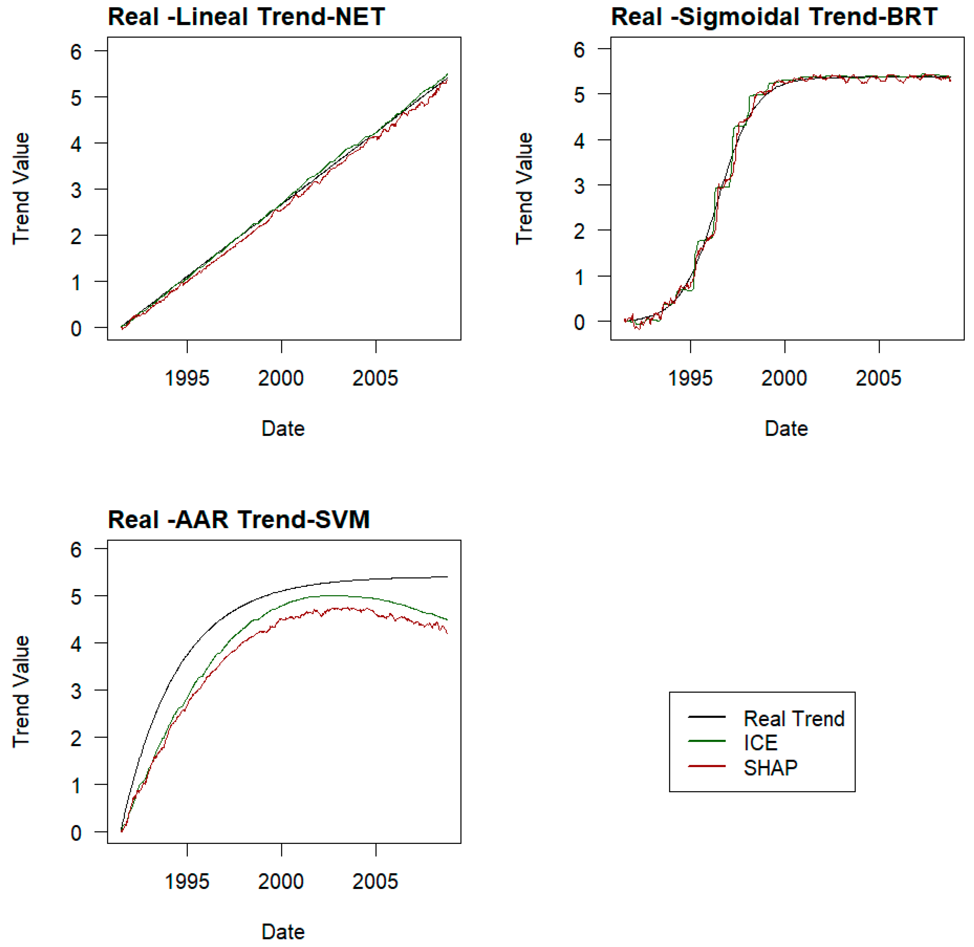
3.5. Extraction of ML Trends

The hypothesis is that the ICE curve with “time” as the mobile explanatory variable, or the SHAP values corresponding to this variable, provides the part of the behaviour captured in the target variable that cannot be explained through the remaining explanatory variables, namely, the part that depends solely on time, the trend.
The determination of the trend based on the ICE curves relative to time in the different models is carried out following the following process.
  • For each record in the dataset, the target variable is predicted with the trained models, while keeping all explanatory variables constant, except for the time variable, which varies throughout its domain in the data set. This provides a set of as many curves as there are records in the dataset, reflecting the variation of the model’s response when only the time variable changes, while keeping the values of the remaining variables fixed for each record.
  • For each value of the time variable in the dataset, the average value of the values obtained for that instant in the set of ICE curves is obtained.
  • The hypothetical trend curve is defined by these averaged values.
In this study, there are strong correlations between explanatory variables, since integrations of level or temperature are used over different time periods. However, the time variable does not show this strong correlation with any of them, and the combinations of values of strongly correlated variables are not altered in the process, making the method of ICE curves applicable. In any case, any doubts are dispelled by observing the procedure’s capability obtained from the test campaign conducted, beyond any theoretical discussion.
SHAP values corresponding to the variable ‘time’ are obtained following this process:
  • For each instance in the dataset, SHAP values are calculated by performing the following actions:
    Evaluating the prediction of the model when the ‘time’ variable is included (active) and when it is excluded (inactive).
    Compare these predictions to determine the impact of the feature.
    Considering all possible combinations of features to ensure fair attribution.
  • The SHAP values for the variable ‘time’ represent the average marginal contribution of this feature across all possible combinations of features.
Trends are determined by both methods on a sample of three experiments in each phase. The RMSE, MAE, and R2 values of the trends obtained are compared with the real ones, and the method that provides the best result is selected.
The trends for the remaining experiments in each phase are determined using the selected method.

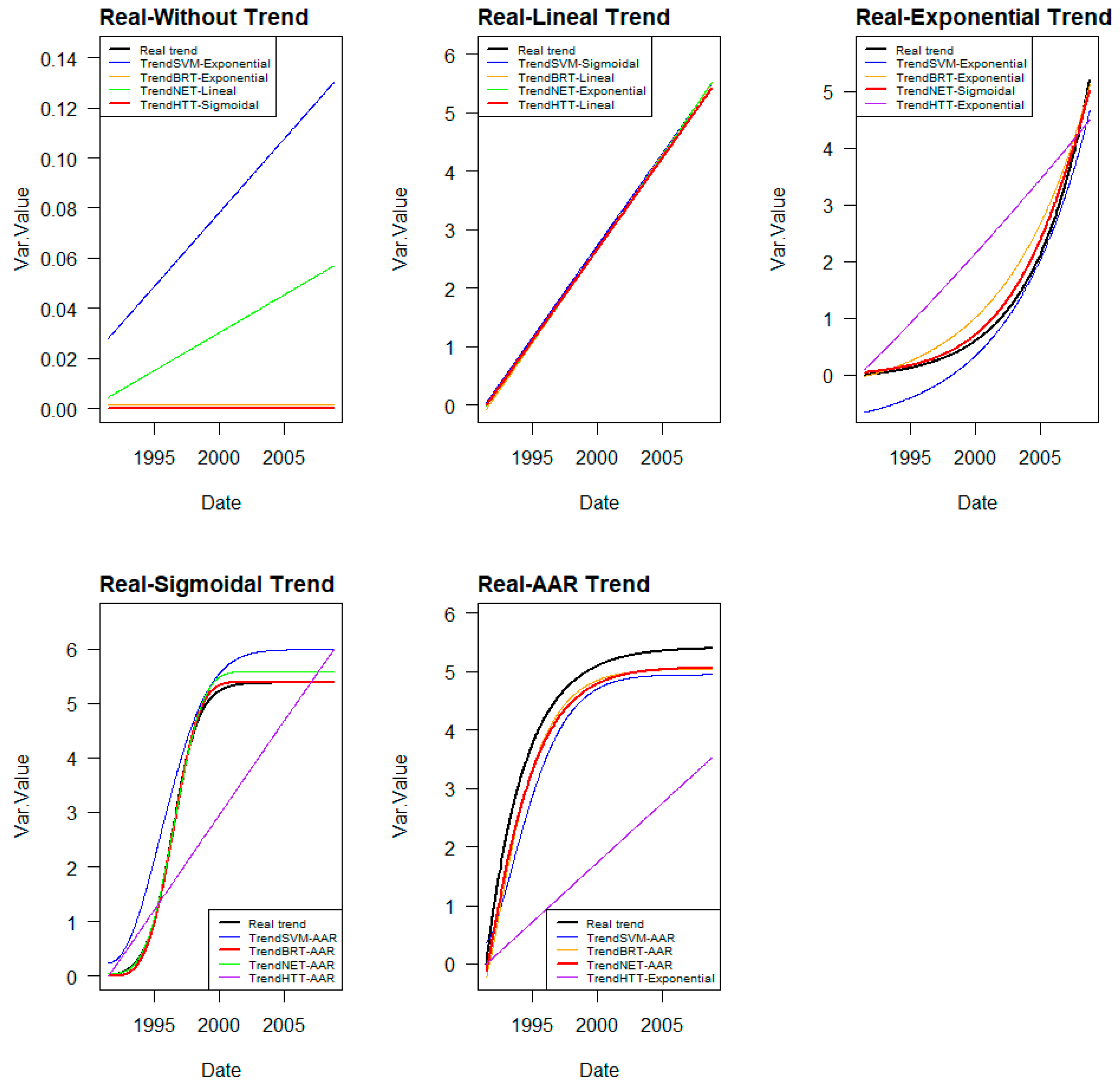
3.6. Adjustment of ML Trend Laws

The trends obtained with each model will be different from each other and will respond to the nature of each model’s algorithm and the relationships found between the explanatory variables and the target variable. While SVMs, by adjusting hyperplanes, or the employed neural networks (perceptron) provide smoother curves, BRT, being based on decision trees, provides stepped lines.
Adjusting these trend lines to the expected, or more common, trends in dam behaviour described in Section 3.2 is carried out with the following coefficients as the variables to be adjusted:
Linear Trend: t l , i = m · T i + k l  Coef.: m, kl
Exponential Trend: t e , i = d · p T i + k e  Coef.: d, p, ke
Sigmoidal Trend: t s , i = q · 1 1 + e T i k 1 k 2 k s  Coef.: q, k1, k2, ks
Expansive Reaction Trend: t r , i = k a + B 1 e T i C p  Coef.: B, p, C, ka
Adjustment of the trend lines to these laws is carried out using the Grey Wolf Optimiser (GWO) algorithm [33]. For each trend extracted from the ML models, the four laws are fitted, and the RMSE, MAE, and R2 of each fit are measured. The trend with the lowest errors and better performance is selected as the most plausible. The correctness of the trend selection is analysed.

3.7. Determining Error in Real Trends

Once the type of law that best fits each trend line extracted from the different ML models is selected, they are compared with the real trends introduced in the base series, measuring RMSE, MAE, and R2.
R M S E = i = 1 n y i ^ y i 2 n
M A E = 1 n i = 1 n y i ^ y i 2
R 2 = 1 i = 1 n y i ^ y i 2 i = 1 n y ¯ y i 2
where y i ^ represents the predicted values, y ¯ represents the mean of the actual values, yi represents the ith actual value, and n is the number of records in the sample.

4. Results and Discussion

In this section, the results obtained from the application of the methodology described to the series comprising the experiments of Phase I and Phase II are presented.

4.1. Phase I Study on Pure Synthetic Series

In Figure 4, the base of the pure synthetic series of the experiments in this phase can be observed, generated from the criteria outlined in Section 3.1.1., and the series obtained by adding them to the trends generated from the expressions described in Section 3.2. In each graph, both the resulting series and the trend employed can be observed.
In each of these series, the four types of predictive models indicated in Section 3.4 are trained. In this way, a total of 20 models are generated, the results of which are presented graphically in Figure 5, along with a summary of the errors committed by each model in Table 3.
The trends obtained using ICE curves and SHAP values on a sample of three experiments in this phase are shown in Figure 6 alongside the corresponding real trend for each experiment.
Table 4 below presents the RMSE, MAE, and R2 values obtained by each of the methods, highlighting in bold the best result in each case. ICE curves provide better results while requiring substantially less computational effort and, therefore, will be used to identify the trend in experiments of this phase.
Using the ICE curves as the best option, the temporal dependency lines of all the experiments in this phase are obtained, as shown in Figure 7, along with the trend line used for each set of models.
The lines of temporal dependence are obtained as the average of the ICE curves of each model, and therefore, the initial value of these curves will generally be different from zero. Considering that, in a behaviour affected by a trend, the irreversible increments that can be observed are relative to the value of the moment when the series begins, the initial value of this trend can be taken as null. For this reason, the initial value of each model’s lines of temporal dependence is subtracted from them so that they start at zero.
On each of these lines of temporal dependence, the adjustment is made to the types of function established according to the methodology described in Section 3.6, and the error of each adjustment is measured with its line of temporal dependence. The one with the lowest RMSE is selected as the best approximation. The table compares the selected fitting laws with the laws actually introduced in each case. In Figure 8, the adjusted laws of temporal dependence with the lowest error are shown for each type of ML model, along with the trend introduced in each case. Table 5 shows the errors made by each fit with respect to the introduced trend.

4.2. Phase II—Study on Series of Real Complexity

In this second phase, the methodology used for Phase I is replicated but applied to the stationary behaviour series described in Section 3.1.2. In this case, the series resulting from the addition of the different trends to the base series can be observed in Figure 9 below.
The results of the prediction models developed in these series provide the results shown in Figure 10 and Table 6.
The trends obtained using ICE curves and SHAP values on a sample of three experiments in this phase are shown in Figure 11 alongside the corresponding real trend for each experiment.
Table 7 below presents the RMSE, MAE, and R2 values obtained by each of the methods, highlighting in bold the best result in each case. ICE curves provide better results while requiring substantially less computational effort and, therefore, will be used to identify the trend in experiments of this phase.
From the trained models and following the method described in Section 3.5 for the ICE curves, the temporal dependence curves are obtained, which can be observed in Figure 12.
The best fits of the different temporal dependence curves to the real trends are shown graphically in Figure 13, and the errors committed are listed in Table 8.

4.3. Discussion of the Results

4.3.1. Regarding the Representativeness of Conditional Expectation Compared to the Trend

The first specific objective of this study was to verify whether the conditional expectation relative to the time variable that can be extracted from the interpretation methods of ML models, considered black-box models, such as ICE curves or SHAP values, were representative of the existing trends in dam monitoring data series derived from the irreversible evolution phenomena of their behaviour.
Experiments conducted on pure synthetic series and series based on the real behaviour of radial movements of a pendulum in a dam reveal that the partial dependencies of the response of ML models with respect to the time variable found using both ICE curves and SHAP values do indeed have a close relationship with the real trends artificially introduced in both phases of the study.
The results obtained show how conditional expectation curves follow a behaviour similar to real trends. From a quantitative perspective, it is observed that the part of the ML model response attributed to the time variable using the interpretation methods employed significantly aligns with the real values. This demonstrates that it is possible to consider these conditional expectations as a representative reference of the real trend that may be integrated into dam behaviour series.
From the comparative study conducted on a sample of three experiments from each phase on the results obtained following the methodology of ICE curves and SHAP values, it is evident that better results are obtained when the former is used. While the morphology and general amplitude of the temporal dependencies found by both methods follow the real trends introduced, the SHAP values present greater local variability and poorer fit than the ICE curves.
An important factor in the results obtained is that there is no strong correlation between the time variable and the rest of the causal variables. In cases where this occurs, the procedure followed by the ICE curves results in the calculation of the model response for combinations of causal variables that cannot occur in reality, which can significantly affect the result. Therefore, extrapolating the validity of the result obtained with the time variable using this method to other explanatory variables and considering that the conditional expectation associated with a strongly correlated variable is a good representation of the dam’s response to that variable may not be valid.

4.3.2. On the Engineering Significance of the Temporal Dependencies Found

The second specific objective was to evaluate whether the conditional expectations obtained respond to the irreversible behaviour characteristics of dams, equivalent to those used to generate trends artificially. In this regard, it is observed that although the ranges and general shapes of the conditional dependencies identified respond to the introduced trends, substantial differences are observed from the dam engineering perspective, necessitating a review of the extracted conditional dependencies for engineering interpretation.
The conditional expectations found in BRT models provide a staggered pattern derived from their own nature based on decision trees. These shapes might suggest an irreversible behaviour of the dam subject to strong punctual increases in movements, which, given that the solution to the problem is known in this study, is not correct.
On the other hand, SVM provides opposite slopes at the ends of the behaviour prediction series compared to the real ones.
Neural networks also show a divergence from the real trends, especially at their final ends.
These behaviours observed in ML behaviour models are particularly evident when there is no trend. In these cases, studying the expected future evolution of the trend would result in significant errors if the result were extrapolated beyond the data cutoff date. In the case of SVM or neural network models, differences in slopes would lead to increasing errors over time or even changes in the trend direction. In the case of BRT models, the results of the conditional expectation for values of the time variable outside the data range would remain constant at their last value.
Given this disparity of results compared to what is expected from an engineering perspective, it becomes necessary to adjust the conditional expectations found to mathematical functions that meet engineering criteria.
It is observed that, once the conditional expectations are adjusted to the shape functions, these problems are logically resolved, resulting in the final trends thus defined being highly representative of the real trends introduced, making them useful for assessing the existing trend.
However, it should be noted that for cases without trends, ML models tend to identify a linear trend, albeit generally with a reduced slope.
The ML models that provide better approximations to real trends, outside of cases without trends or with linear trends, are BRT and neural networks. Although the overall accuracy of SVM models is not much worse than that of the others, it is penalised by the interpretations it makes at the ends of the prediction series.
In general, the type of formula that best fits is the same as that that defines the trend. However, in the case of exponential trends, both in Phase I and in Phase II, sigmoidal-type trend formulas best fit. For the conditional expectations found by the SVM and BRT models, however, the best fit is achieved using the exponential function in both cases.
In the case of sigmoidal trends, in phase II, the best fit was achieved with an AAR-type function. Note that both formulations respond to a sigmoidal-type function.

4.3.3. On the Comparison of Results Obtained with the Most Common Statistical Methods in Dam Safety

It is observed that, for cases without trends or with linear trends, it is the HTT-type multiple linear regression model that provides a perfect fit both in prediction and trend. This is because the carrier series of the two phases were created from HTT models with the same term structure. Since the form imposed on the response model incorporates the specific terms of a linear trend, it is logical that in these two cases, the fit is perfect.
In these cases, ML models, although logically worse than HTT, provide a fairly similar overall fit of the trend, with little impact on the study period, but with types of fit formulas, sometimes, different from the real ones.
However, when the introduced trend deviates from a straight line, we see how the restrictions imposed by the polynomial structure on HTT have a greater impact on trend identification. It is observed that in these cases, HTT models assign almost straight alignments to the temporal part of the behaviour, deviating significantly from the real trend in these cases. The trends obtained from the ML models clearly fit more closely to the real trends, thus showing significantly greater utility for detecting and defining trends in dam behaviour.

4.3.4. Limitations of Methodology and Future Research Lines

In both phases of the study, trained ML models provide good predictions, as reflected in the errors and R2 obtained. This provides an indication of how well the regressors employed are able to explain the modelled behaviour. In real cases, sometimes, the information necessary for explaining the modelled behaviours is not complete or sufficiently precise, resulting in vaguer behaviour models. The conditional expectation extracted from these models may then be influenced and lose representativeness. Therefore, further research is needed to study the impact of the quality of ML models on trend identification.

5. Conclusions

Through this study, it was demonstrated how the conditional expectation relative to the time variable extracted from ML models that predict dam behavior responds to the existing trend.
It has been verified that it is possible to define the trend in the series consistent with the knowledge of dam engineering by adjusting the conditional expectations extracted from the models to mathematical functions corresponding to different types of known irreversible phenomena in dams.
The greater versatility and detection capability of this method were evidenced compared to common practices used in dam safety.
Therefore, the proposed methodology provides a useful tool for dam safety experts in identifying, defining, and studying the irreversible phenomena to which a dam can be subjected, which is fundamental to its safety.

Author Contributions

Conceptualisation, M.Á.F.-C., P.A. and M.Á.T.; methodology, M.Á.F.-C.; software, M.Á.F.-C.; formal analysis, M.Á.F.-C., P.A. and M.Á.T.; investigation, M.Á.F.-C.; data curation, M.Á.F.-C.; writing—original draft preparation, M.Á.F.-C.; writing—review and editing, P.A. and M.Á.T.; visualization, M.Á.F.-C.; supervision, M.Á.T. All authors have read and agreed to the published version of the manuscript.

Funding

This research was funded by the program NEOTEC of the Center for Industrial Technological Development (CDTI), an organization under the Ministry of Science and Innovation of the Government of Spain. (SNEO—20211264 TECNOLOGÍA EFICIENTE PARA LA SEGURIDAD DE OBRAS HIDRÁULICAS).

Data Availability Statement

Third Party Data: Restrictions apply to the availability of these data. Data were obtained from Agència Catalana de l’Aigua (ACA) and are available from the authors with the permission of ACA.

Acknowledgments

The authors thank Agència Catalana de l’Aigua (ACA) for providing the data.

Conflicts of Interest

Miguel Á. Fernández-Centeno and Patricia Alocén are doctoral students at UPM and work at ACIS Innovation + Engineering S.L., a spin-off of UPM. The remaining authors declare that the research was conducted in the absence of any commercial or financial relationships that could be construed as a potential conflict of interest.

Nomenclature

AARAggregate Alkali Reaction
AIArtificial Intelligence
AARAggregate Alkali Reaction
ALEAccumulated Local Effects
ANN, NN, NETNeural Networks
BRTBoosted Regression Trees
CVCross-Validation
DLDeep Learning
GWOGrey Wolf Optimiser
HTTHydrostatic-Temperature-Time
ICEIndividual Conditional Expectation
MAEMean Absolute Error
MLMachine Learning
R2Coefficient of Determination
RMSERoot-Mean-Square Error,
SVMSupport Vector Machine

References

  1. Saplıoğlu, K.; Güçlü, Y.S. Combination of Wilcoxon test and scatter diagram for trend analysis of hydrological data. J. Hydrol. 2022, 612, 128132. [Google Scholar] [CrossRef]
  2. Mehta, D.J.; Yadav, S. Long-term trend analysis of climate variables for arid and semi-arid regions of an Indian State Rajasthan. Int. J. Hydrol. Sci. Technol. 2022, 13, 191–214. [Google Scholar] [CrossRef]
  3. Wang, Y.; Xu, Y.; Tabari, H.; Wang, J.; Wang, Q.; Song, S.; Hu, Z. Innovative trend analysis of annual and seasonal rainfall in the Yangtze River Delta, eastern China. Atmospheric Res. 2020, 231, 104673. [Google Scholar] [CrossRef]
  4. Loh, C.-H.; Chen, C.-H.; Hsu, T.-Y. Application of advanced statistical methods for extracting long-term trends in static monitoring data from an arch dam. Struct. Health Monit. 2011, 10, 587–601. [Google Scholar] [CrossRef]
  5. Liu, X.; Li, Z.; Sun, L.; Khailah, E.Y.; Wang, J.; Lu, W. A critical review of statistical model of dam monitoring data. J. Build. Eng. 2023, 80, 108106. [Google Scholar] [CrossRef]
  6. Mata, J.; Gomes, J.P.; Pereira, S.; Magalhães, F.; Cunha, Á. Analysis and interpretation of observed dynamic behaviour of a large concrete dam aided by soft computing and machine learning techniques. Eng. Struct. 2023, 296, 116940. [Google Scholar] [CrossRef]
  7. Li, W.; Wu, Z. A methodology for dam parameter identification combining machine learning, multi-objective optimization and multiple decision criteria. Appl. Soft Comput. 2022, 128, 109476. [Google Scholar] [CrossRef]
  8. Li, M.; Ren, Q.; Li, H.; Song, L. DRLSTM: A dual-stage deep learning approach driven by raw monitoring data for dam displacement prediction. Adv. Eng. Inform. 2022, 51, 101510. [Google Scholar] [CrossRef]
  9. Li, M.; Pan, J.; Liu, Y.; Liu, H.; Wang, J.; Zhao, Z. A deformation prediction model of high arch dams in the initial operation period based on PSR-SVM-IGWO. Math. Probl. Eng. 2021, 2021, 8487997. [Google Scholar] [CrossRef]
  10. Li, M.; Pan, J.; Liu, Y.; Wang, Y.; Zhang, W.; Wang, J. Dam deformation forecasting using SVM-DEGWO algorithm based on phase space reconstruction. PLoS ONE 2022, 17, e0267434. [Google Scholar] [CrossRef] [PubMed]
  11. Salazar, F.; Hariri-Ardebili, M.A. Coupling machine learning and stochastic finite element to evaluate heterogeneous concrete infrastructure. Eng. Struct. 2022, 260, 114190. [Google Scholar] [CrossRef]
  12. Salazar, F.; Toledo, M.; Oñate, E.; Morán, R. An empirical comparison of machine learning techniques for dam behaviour modelling. Struct. Saf. 2015, 56, 9–17. [Google Scholar] [CrossRef]
  13. Cortez, P.; Embrechts, M.J. Using sensitivity analysis and visualization techniques to open black box data mining models. Inf. Sci. 2013, 225, 1–17. [Google Scholar] [CrossRef]
  14. Lin, C.; Chen, S.; Hariri-Ardebili, M.A.; Li, T. An Explainable Probabilistic Model for Health Monitoring of Concrete Dam via Optimized Sparse Bayesian Learning and Sensitivity Analysis. Struct. Control. Health Monit. 2023, 2023, 2979822. [Google Scholar] [CrossRef]
  15. Lundberg, S.M.; Lee, S.-I. A unified approach to interpreting model predictions. In Advances in Neural Information Processing Systems; Curran Associates, Inc.: New York, NY, USA, 2017; Volume 30. [Google Scholar]
  16. Shao, L.; Wang, T.; Wang, Y.; Wang, Z.; Min, K. A Prediction Model and Factor Importance Analysis of Multiple Measuring Points for Concrete Face Rockfill Dam during the Operation Period. Water 2023, 15, 1081. [Google Scholar] [CrossRef]
  17. Tursunalieva, A.; Alexander, D.L.J.; Dunne, R.; Li, J.; Riera, L.; Zhao, Y. Making Sense of Machine Learning: A Review of Interpretation Techniques and Their Applications. Appl. Sci. 2024, 14, 496. [Google Scholar] [CrossRef]
  18. Ribeiro, M.T.; Singh, S.; Guestrin, C. ‘Why should I trust you?’ Explaining the predictions of any classifier. In Proceedings of the 22nd ACM SIGKDD International Conference on Knowledge Discovery and Data Mining, San Francisco, CA, USA, 13–17 August 2016; pp. 1135–1144. [Google Scholar]
  19. Selvaraju, R.R.; Cogswell, M.; Das, A.; Vedantam, R.; Parikh, D.; Batra, D. Grad-CAM: Visual explanations from deep networks via gradient-based localization. In Proceedings of the 2017 IEEE International Conference on Computer Vision (ICCV), Venice, Italy, 22–29 October 2017; pp. 618–626. [Google Scholar] [CrossRef]
  20. Goldstein, A.; Kapelner, A.; Bleich, J.; Pitkin, E. Peeking Inside the Black Box: Visualizing Statistical Learning With Plots of Individual Conditional Expectation. J. Comput. Graph. Stat. 2015, 24, 44–65. [Google Scholar] [CrossRef]
  21. Štrumbelj, E.; Kononenko, I. Explaining prediction models and individual predictions with feature contributions. Knowl. Inf. Syst. 2013, 41, 647–665. [Google Scholar] [CrossRef]
  22. Yeh, A.; Ngo, A. Bringing a Ruler Into the Black Box: Uncovering Feature Impact from Individual Conditional Expectation Plots. In Machine Learning and Principles and Practice of Knowledge Discovery in Databases; Kamp, M., Koprinska, I., Bibal, A., Bouadi, T., Frénay, B., Galárraga, L., Oramas, J., Adilova, L., Krishnamurthy, Y., Knag, B., et al., Eds.; Springer International Publishing: Cham, Switzerland, 2021; pp. 34–48. [Google Scholar]
  23. Apley, D.W.; Zhu, J. Visualizing the Effects of Predictor Variables in Black Box Supervised Learning Models. J. R. Stat. Soc. Ser. B (Statistical Methodol. 2020, 82, 1059–1086. [Google Scholar] [CrossRef]
  24. Baucells, M.; Borgonovo, E.; Plischke, E.; Barr, J.; Rabitz, H. Trend Analysis in the Age of Machine Learning; UVA Darden School of Business: Charlottesville, VA, USA, 2021. [Google Scholar]
  25. Salazar, F.; Toledo, M.; Oñate, E.; Suárez, B. Interpretation of dam deformation and leakage with boosted regression trees. Eng. Struct. 2016, 119, 230–251. [Google Scholar] [CrossRef]
  26. Hu, J.; Ma, F. Comparison of hierarchical clustering based deformation prediction models for high arch dams during the initial operation period. J. Civ. Struct. Health Monit. 2021, 11, 897–914. [Google Scholar] [CrossRef]
  27. Cunha, J.; Faria, A.; Mata, J.; Salazar, F. Use of boosted regression tree algorithms in dam behavior analysis. Case of Covão do Meio dam (Portugal). In Proceedings of the Symposium “Management for Safe Dams”—91st Annual ICOLD Meeting, Gothenburg, Sweden, 13–14 June 2023. [Google Scholar]
  28. Wang, S.; Sui, X.; Liu, Y.; Gu, H.; Xu, B.; Xia, Q. Prediction and interpretation of the deformation behaviour of high arch dams based on a measured temperature field. J. Civ. Struct. Health Monit. 2023, 13, 661–675. [Google Scholar] [CrossRef]
  29. Yin, L.; Wang, L.; Li, T.; Lu, S.; Tian, J.; Yin, Z.; Li, X.; Zheng, W. U-Net-LSTM: Time Series-Enhanced Lake Boundary Prediction Model. Land 2023, 12, 1859. [Google Scholar] [CrossRef]
  30. Léger, P.; Leclerc, M. Hydrostatic, Temperature, time-displacement model for concrete dams. J. Eng. Mech. 2007, 133, 267–277. [Google Scholar] [CrossRef]
  31. Mata, J.; de Castro, A.T.; da Costa, J.S. Constructing statistical models for arch dam deformation. Struct. Control Health Monit. 2014, 21, 423–437. [Google Scholar] [CrossRef]
  32. Araujo, G.S.; de Cea, A.A.; Fité, L.A.; Yepes, S.C.; Iglesias, F.R. Estudio del comportamiento de presas de hormigón frente al ataque sulfático. In Las Estructuras del Siglo XXI, Sostenibilidad, Innovación y Retos del Futuro: Comunicaciones; Asociación Española de Ingeniería Estructural (ACHE): Madrid, Spain, 2005; pp. 1433–1445. [Google Scholar]
  33. Mirjalili, S.; Mirjalili, S.M.; Lewis, A. Grey Wolf Optimizer. Adv. Eng. Softw. 2014, 69, 46–61. [Google Scholar] [CrossRef]
Figure 1. Proposed methodology scheme.
Water 16 01239 g001
Figure 2. Pure synthetic stationary series appearance.
Water 16 01239 g002
Figure 3. Behaviour-based stationary series appearance
Water 16 01239 g003
Figure 4. Pure synthetic series and Applied Trends. The pure synthetic series corresponding to the different experiments in Phase I can be observed in grey. Each of these series is the sum of the pure synthetic series for the “Without Trend” case and the introduced trend, which is plotted in black for each case.
Water 16 01239 g004
Figure 5. Predictions obtained with the different models trained on each Phase I experiment. Poorer performance of the HTT models can be observed in cases of non-linear trends. The models corresponding to the exponential trend case show a lower accuracy at the end of the series.
Water 16 01239 g005
Figure 6. Conditional expectation relative to time variable, or trends, obtained using ICE curves and SHAP values in a sample of three experiments of Phase I. Lower local variability and better fit to real trend can be observed in the trends obtained with ICE curves.
Water 16 01239 g006
Figure 7. Real trends and lines of conditional expectation with respect to the time variable obtained in each of the ML and HTT models trained for each experiment in Phase I.
Water 16 01239 g007
Figure 8. Real trends and best fits to typical irreversible behaviour functions of dams for each type of ML and HTT model trained for each of the experiments in Phase I. The best fit to the real trend of each case is highlighted in thicker red lines.
Water 16 01239 g008
Figure 9. Behaviour-based stationary series and Applied Trends. The behaviour-based stationary series corresponding to the different experiments in Phase II can be observed in grey. Each of these series is the sum of the pure synthetic series for the “Without Trend” case and the introduced trend, which is plotted in black for each case.
Water 16 01239 g009
Figure 10. Predictions obtained with the different models trained in each Phase II experiment. Poorer performance of the HTT models can be observed in cases of non-linear trends.
Water 16 01239 g010
Figure 11. Conditional expectation relative to time variable, or trends, obtained using ICE curves and SHAP values in a sample of three experiments of Phase II. Lower local variability and better fit to the real trend can be observed in the trends obtained with the ICE curves.
Water 16 01239 g011
Figure 12. Real trends and lines of conditional expectation with respect to the time variable obtained in each of the ML and HTT models trained for each experiment in Phase II.
Water 16 01239 g012
Figure 13. Real trends and best fits to typical irreversible behaviour functions of dams for each type of ML and HTT model trained for each of the experiments in Phase II. The best fit to the real trend of each case is highlighted in thicker red lines.
Water 16 01239 g013
Table 1. Data Statistics of the pure synthetic stationary series
Min.1st Qu.MedianMean3rd Qu.Max.SD
−17.641−7.288−3.528−0.940−0.24232.00612.486
Table 2. Data Statistics of the behaviour-based stationary series
Min.1st Qu.MedianMean3rd Qu.Max.SD
−8.829−6.527−4.848−4.864−3.4890.5492.030
Table 3. RMSE, MAE, and R2 calculated for each of the ML and HTT models trained on the different experiments of Phase I. The best ML model for each type of trend is highlighted in bold.
Without TrendLinear TrendExponential TrendSigmoidal TrendAAR Trend
RMSEMAER2RMSEMAER2RMSEMAER2RMSEMAER2RMSEMAER2
SVM0.8240.7120.9961.0570.9320.9961.7461.1550.9871.1790.9530.9961.1330.8810.995
BRT0.0010.0001.0001.9821.6750.9933.0051.6030.9631.9671.4550.9892.4051.6120.983
NET0.1540.1111.0000.8070.6230.9981.6910.9440.9880.6520.4920.9990.9840.6710.996
HTT0.0000.0001.0000.0000.0001.0005.9574.4020.8313.2312.8940.9663.4042.9320.947
Table 4. RMSE, MAE, and R2 of the trends obtained using the ICE curves and SHAP values in Phase I with respect to the real trend artificially introduced in the data series. It can be observed that the results provided by the ICE curves improve in almost all cases compared to those obtained with the SHAP values. The best performance indexes are highlighted in bold.
TypeTrend TypeModel TypeICESHAP
RMSEMAER2RMSEMAER2
PAABRT1.2310.8550.9911.5671.4600.996
PEXNET0.4240.2650.9981.3481.0240.972
PSGSVM1.1240.9220.9972.4992.0360.986
Table 5. RMSE, MAE, and R2 of the fits to the different types of functions representing potentially expected irreversible behaviour patterns in dam data, according to engineering criteria, of the lines of conditional expectation relative to the time variable determined by each ML and HTT model trained in each of the experiments corresponding to Phase I. The best fit of each model type has been highlighted in bold, and the fit with the lowest error and model has been underlined in grey.
Without Trend
ModelLinear AdjustmentExponential AdjustmentSigmoidal AdjustmentAAR Adjustment
RMSEMAER2RMSEMAER2RMSEMAER2RMSEMAER2
SVM0.3310.331 0.3320.332 0.3420.332 0.3460.335
BRT0.0000.000 0.0000.000 0.0000.000 0.0000.000
NET0.0550.051 0.0490.044 0.0540.051 0.0530.049
HTT0.0000.000 0.0000.000 0.0000.000 0.0000.000
Linear Trend
ModelLinear AdjustmentExponential AdjustmentSigmoidal AdjustmentAAR Adjustment
RMSEMAER2RMSEMAER2RMSEMAER2RMSEMAER2
SVM0.2770.2681.0000.2690.2591.0000.2810.2711.0000.2790.2541.000
BRT0.7140.7141.0000.7130.7121.0000.7100.7101.0000.7360.7211.000
NET1.6961.6701.0001.6091.5811.0009.6268.304 1.9251.8380.997
HTT0.0000.0001.0000.1570.1311.0000.0190.0161.0000.0980.0821.000
Exponential Trend
ModelLinear AdjustmentExponential AdjustmentSigmoidal AdjustmentAAR Adjustment
RMSEMAER2RMSEMAER2RMSEMAER2RMSEMAER2
SVM5.4883.1690.6840.4580.3171.0000.6960.4960.9950.7110.5290.995
BRT5.8093.2010.6840.7640.4901.0000.9300.5971.0000.9550.6130.997
NET5.0463.1430.6844.8593.1530.6870.4100.2260.9980.5870.4010.994
HTT4.9813.4070.7094.8903.3330.7234.9703.3980.7105.0023.4260.706
Sigmoidal Trend
ModelLinear AdjustmentExponential AdjustmentSigmoidal AdjustmentAAR Adjustment
RMSEMAER2RMSEMAER2RMSEMAER2RMSEMAER2
SVM3.0922.5930.9513.0522.5750.9521.1250.9580.9971.1330.9730.997
BRT2.8572.5240.9512.8522.4970.9510.4540.3560.9990.8110.5900.998
NET2.9452.5900.9512.9102.5590.9521.7131.4440.9901.6871.3680.990
HTT3.1512.6110.9573.1592.6050.9563.1502.6140.9573.0442.5110.962
AAR Trend
ModelLinear AdjustmentExponential AdjustmentSigmoidal AdjustmentAAR Adjustment
RMSEMAER2RMSEMAER2RMSEMAER2RMSEMAER2
SVM3.2372.7100.8623.3432.7180.8581.1641.1431.0001.1891.1430.999
BRT3.2382.6810.8623.2732.7130.8580.8560.7351.0000.7600.6740.999
NET3.2992.5170.8623.4832.5550.8560.1720.1231.0000.1600.1181.000
HTT4.2243.3410.8764.3263.3590.8634.2213.3410.8764.2033.3300.878
Table 6. RMSE, MAE, and R2 calculated for each of the ML and HTT models trained on the different experiments of Phase II. The best ML model for each type of trend is highlighted in bold.
Without TrendLinear TrendExponential TrendSigmoidal TrendAAR Trend
RMSEMAER2RMSEMAER2RMSEMAER2RMSEMAER2RMSEMAER2
SVM0.1420.1240.9950.1940.1680.9960.2630.2100.9910.4680.3870.9810.2910.2240.989
BRT0.1420.1080.9950.3290.2570.9900.3720.2640.9850.3460.2490.9900.2950.2100.989
NET0.1040.0770.9970.1320.0930.9980.2670.1790.9910.2510.1820.9950.2340.1640.993
HTT0.0000.0001.0000.0000.0001.0000.7370.6000.9291.2011.0970.8750.8020.6590.914
Table 7. RMSE, MAE, and R2 of the trends obtained using the ICE curves and SHAP values in Phase II with respect to the real trend artificially introduced in the data series. A generally better outcome of ICE curves can be observed compared to SHAP values. The best performance indexes are highlighted in bold.
TypeTrend TypeModel TypeICESHAP
RMSEMAER2RMSEMAER2
MLINET0.0500.0391.0000.1100.1040.999
MSGBRT0.1540.1020.9950.1250.0850.997
MAASVM0.5940.5500.9750.8180.7940.976
Table 8. RMSE, MAE, and R2 of the fits to the different types of functions representing potentially expected irreversible behaviour patterns in dam data, according to engineering criteria, of the lines of conditional expectation relative to the time variable determined by each ML and HTT model trained in each of the experiments corresponding to Phase II. The best fit of each model type has been highlighted in bold, and the fit with the lowest error and model has been underlined in grey.
Without Trend
ModelLinear AdjustmentExponential AdjustmentSigmoidal AdjustmentAAR Adjustment
RMSEMAER2RMSEMAER2RMSEMAER2RMSEMAER2
SVM0.0840.080 0.0840.078 0.0850.078 0.0840.078
BRT0.0070.006 0.0020.002 0.0070.006 0.0080.007
NET0.0340.030 0.0340.030 0.0340.030 0.0340.030
HTT0.0000.000 0.0000.000 0.0000.000 0.0000.000
Linear Trend
ModelLinear AdjustmentExponential AdjustmentSigmoidal AdjustmentAAR Adjustment
RMSEMAER2RMSEMAER2RMSEMAER2RMSEMAER2
SVM0.0690.0681.0000.0970.0891.0000.0690.0681.0000.1160.1000.999
BRT0.0450.0381.0000.0500.0431.0000.0450.0381.0000.2500.2170.984
NET0.0400.0331.0000.0390.0271.0000.0400.0331.0000.0490.0431.000
HTT0.0000.0001.0000.0370.0300.9990.0040.0031.0000.0030.0021.000
Exponential Trend
ModelLinear AdjustmentExponential AdjustmentSigmoidal AdjustmentAAR Adjustment
RMSEMAER2RMSEMAER2RMSEMAER2RMSEMAER2
SVM0.7850.5820.8100.3830.3370.9870.3980.3610.9900.3870.3370.986
BRT0.6410.4920.8100.3560.3030.9820.3560.3030.9820.3890.3140.978
NET0.6090.4790.8100.6080.4790.8100.1410.1190.9960.1570.1300.995
HTT1.1571.0360.8101.1471.0360.8301.1571.0360.8101.1581.0360.810
Sigmoidal Trend
ModelLinear AdjustmentExponential AdjustmentSigmoidal AdjustmentAAR Adjustment
RMSEMAER2RMSEMAER2RMSEMAER2RMSEMAER2
SVM1.1491.0060.7621.1531.0090.7601.1501.0060.7620.6230.5710.986
BRT1.0850.9170.7621.0880.9190.7620.5350.3960.9350.0510.0391.000
NET1.0650.9130.7621.0780.9280.7560.6310.4840.9140.1700.1420.999
HTT1.3091.0300.7621.3101.0310.7621.3121.0350.7591.3071.0270.764
AAR Trend
ModelLinear AdjustmentExponential AdjustmentSigmoidal AdjustmentAAR Adjustment
RMSEMAER2RMSEMAER2RMSEMAER2RMSEMAER2
SVM0.8480.7150.6810.8500.7170.6810.8480.7150.6810.5700.5330.978
BRT0.8180.6460.6810.8250.6510.6720.8180.6460.6810.3740.3540.997
NET0.8250.6170.6810.8250.6170.6791.3100.8940.0000.3700.3620.998
HTT2.8232.7290.6812.8222.7280.6812.8232.7280.6782.8232.7290.681
Disclaimer/Publisher’s Note: The statements, opinions and data contained in all publications are solely those of the individual author(s) and contributor(s) and not of MDPI and/or the editor(s). MDPI and/or the editor(s) disclaim responsibility for any injury to people or property resulting from any ideas, methods, instructions or products referred to in the content.

