
A Multi-Satellite SBAS for Retrieving Long-Term Ground Displacement Time Series

1
Department of Land Surveying and Geo-Informatics, Hong Kong Polytechnic University, Hong Kong, China
2
Department of Geomatics Engineering, Faculty of Engineering at Shoubra, Benha University, Cairo 11672, Egypt
*
Author to whom correspondence should be addressed.
Remote Sens. 2024, 16(9), 1520; https://0-doi-org.brum.beds.ac.uk/10.3390/rs16091520
Submission received: 15 February 2024
/
Revised: 17 April 2024
/
Accepted: 22 April 2024
/
Published: 25 April 2024
(This article belongs to the Section Environmental Remote Sensing)
Abstract
:Ground deformation is one of the crucial issues threatening many cities in both societal and economic aspects. Interferometric synthetic aperture radar (InSAR) has been widely used for deformation monitoring. Recently, there has been an increasing availability of massive archives of SAR images from various satellites or sensors. This paper introduces Multi-Satellite SBAS that exploits complementary information from different SAR data to generate integrated long-term ground displacement time series. The proposed method is employed to create the vertical displacement maps of Almokattam City in Egypt from 2000 to 2020. The experimental results are promising using ERS, ENVISAT ASAR, and Sentinel-1A displacement integration. There is a remarkable deformation in the vertical direction along the west area while the mean deformation velocity is −2.32 mm/year. Cross-validation confirms that the root mean square error (RMSE) did not exceed 2.8 mm/year. In addition, the research findings are comparable to those of the previous research in the study area. Consequently, the proposed integration method has great potential to generate displacement time series based on multi-satellite SAR data; however, it still requires further evaluation using field measurements.
1. Introduction
In recent years, megacities have encountered challenges due to ground subsidence which substantially affects human lives and economic expansion. Thus, frequent deformation monitoring is crucial [1]. Interferometric synthetic aperture radar (InSAR) has revolutionized ground deformation monitoring due to high-resolution measurements over large areas in a cost-effective and timely manner. Though traditional techniques (e.g., GPS and leveling) provide precise measurements, they are often limited in their spatial resolution and prohibitively costly for widespread monitoring [2]. On the one hand, differential interferometric synthetic aperture radar (DInSAR) has been shown a powerful tool for monitoring land displacement fields [3] because of day-night and all-weather operation, large-scale coverage, spatial continuity, and high-accuracy measurements [4]. Accordingly, DInSAR has been widely utilized in various disciplines such as volcanology, tectonics, and studies of deformation in urban areas and subsurface utilities [5]. On the other hand, DInSAR, however, has limitations in monitoring long-term time series of Earth’s surface deformation [6]. Therefore, various researchers have developed Multi-Temporal DInSAR techniques to study the temporal growth of land deformation and map ground deformation. This reduced space-time decorrelation in traditional DInSAR techniques [7]. Three main classes were proposed: the persistent scatterer (PS), the distributed scatterer (DS), and combining both approaches [8]. Initially, the PS class utilizes the pixels of the highest resolution while focusing on points containing a single dominant scatterer [9]. Examples of PS class include persistent Scatterer approach [10,11], Stanford Method for Persistent Scatterers Network (StaMPS) [12], Interferometric Point Target Analysis (IPTA) [13], and Spatio-Temporal Unwrapping Network [14]. Secondly, the DS class employs the Small BAseline Subset (SBAS) technique [15], the Coherent Point Target Analysis (CPTA) [16], and the combined technique [17]. These techniques are enhanced for pixel resolution based on scatterer distribution. Finally, the third class combines approaches from PS and DS. Examples of this class include the Enhanced Spatial Differences (ESD) [18], StaMPS, and SqueeSAR.
In the past decade, several SAR satellites have been deployed which enriched the accessibility of data characterizing different wavelengths, angle geometries, and acquisition modes. Consequently, integrating such multi-satellite SAR data with complement characteristics would provide a vast amount of information [19]; however, such integration over non-overlapping periods is challenging [20]. Earlier integration attempts focused only on computing the three-dimensional (3D) ground deformation by either five categories: (1) a combination of at least three DInSAR sensors or track algorithms [4,21,22,23,24,25,26]; (2) fusion of DInSAR and multiple aperture interferometry (MAI) which measures the north-south (NS) components of the average deformation velocity, which cannot be detected from radar satellites of near-polar orbits. In addition, the fusion of MAI and standard DInSAR provides 3D displacement components across broad areas [27,28]; (3) a combination of DInSAR and Pixel Offset (PO) tracking. Such a combination addressed the poor sensitivity of line-of-sight (LOS) measurements to NS displacements [29,30]; (4) InSAR and global navigation satellite system (GNSS) data integration [9,31,32]; (5) Using DInSAR in conjunction with an a priori deformation model [33,34,35].
These approaches have been extended to generate 3D time series displacement such as Pixel-Offset SBAS (PO-SBAS) technology [36]. In addition, Pepe et al. [19] introduced the Minimum Acceleration integration system to augment PO-SBAS; however, it requires appropriate time-overlapped ascending and descending SAR data. Moreover, Hu et al. [23] integrated DInSAR based on the Kalman filter. Therefore, multi-satellite interferograms have been integrated from different orbital positions to retrieve East-West (EW) and Up-Down displacement time series. It is worth noting that such strategies neglected the NS deformation whereas the temporal changeable components of the deformation field have been retained. Further, Samsonov and d’Oreye [37] proposed Multidimensional SBAS (MSBAS) that involved processing a huge number of multi-satellite differential SAR interferograms. Another update of MSBAS integrated the LOS displacement time series from an individual set of SAR data frames [38]. MSBAS does not inherently necessitate simultaneous processing of multi-satellite SAR data. Additionally, MSBAS does not impose any constraints related to recovering the LOS DInSAR time series. Samsonov and Blais-Stevens [39] applied the MSBAS-2D and MSBAS-3D techniques to map two areas in northern Canada where multiple large slow-moving deep-seated landslides were reported using freely—available Sentinel-1 SAR data collected between 2017 and 2022. Tao et al. [40] constructed and solved the Tikhonov regularized 2D deformation models of MSBAS InSAR with three different orders and three different parameters, processed a large number of ascending and descending Sentinel-1A/B SAR images covering a mine, and examined the sensitivity and reliability of the MSBAS regularization methods for estimating vertical and east-west surface deformation time series over the mine by comparing with leveling-monitoring results. Zhao et al. [20] developed modified quantile-quantile adjustment (MQQA) which conducts time-overlapped ground time series deformation while the non-overlapped data were integrated based on an exterior time-dependent model [19]. Furthermore, a modified quantile-quantile adjustment was developed by [20]. In this study, the time-overlapped ground time series deformation was included in the MQQA process whereas an exterior time-dependent model was employed to integrate the non-overlapping data [19]. Tang et al. [41] proposed a method to retrieve the full three-dimensional (3D) displacement field over the oilfield. Specifically, they retrieved the north-south component based on the assumption of a physical relationship between the horizontal and vertical displacement, and they retrieved the vertical and east-west displacement components by combining the multiple-geometry InSAR line-of-sight (LOS) observations. Consistent displacement rate maps and displacement time series in the LOS direction were produced by processing two ascending and two descending datasets from the Sentinel-1 satellite covering the region using an InSAR time series analysis conducted between 2017 and 2021.
From the aforementioned, two key challenges are associated with deriving ground displacement based on multi-satellite SAR data. The first is employing an external time-dependent model to predict the deformation of non-overlapping data. The other is the simultaneous processing of hundreds of differential SAR interferograms. This research presents Multi-Satellite SBAS which is an adaptation of the traditional SBAS. The long-term deformation time series has been generated based on the extended sequences of time-overlapped and time-gapped SAR data without any external deformation model. Additionally, Multi-Satellite SBAS exploits the complementary nature of multi-satellite SAR data with a small number of SAR images. This is expected to perform in areas with moderate-to-low coherence and low-to-no temporal overlapping datasets.
The remainder of this paper is structured as follows: Section 2 explains the study area, dataset, and the proposed research methodology. Section 3 presents the research findings and results. Section 4 discusses the relevant research and the method’s performance. Finally, the conclusions are summarized in Section 5.
2. Materials and Methods
2.1. Materials
2.1.1. Study Area
Almokattam City, located in the Arab Republic of Egypt, is the study area of this research as shown in Figure 1a. The city lies on the upper plateau of the Almokattam mountain in east Cairo. The city has a plateau-like structure with an approximate surface area of 14 km2. The heights above the mean sea level extend from 60 m to roughly 140 m to the east. Layers of the city are convex in the immediate vicinity and heights continue rising to ≈240 m near the castle lowering to the north until ending at the Mountain of Al Amir near Abbasiyah. Notably, Almokattam City has witnessed sustained urbanization over the last decade as shown in Figure 1b–d. The city has seen continuous population growth despite frequent collapses in the Zbaleen, the southwestern scarp of the high plateau, and Manshiat Nasser. Consequently, the rocks in Almokattam City exhibit instability and are continually prone to potential collapses [42,43,44].
2.1.2. Dataset
This research has proposed a method to integrate multi-satellite SAR data from three independent datasets to retrieve the ground displacement. Set I: ENVISAT ASAR data covering the period from 2008 to 2012. Set II: European Remote Sensing satellite (ERS) SAR images acquired from 2000 to 2010. Lastly, set III: European Union Sentinel-1A (S1) images collected from 2014 to 2020. Table 1 lists the characteristics of each dataset. Also, Figure 1b shows the spatial coverage of the datasets over the study area.
2.2. Methods
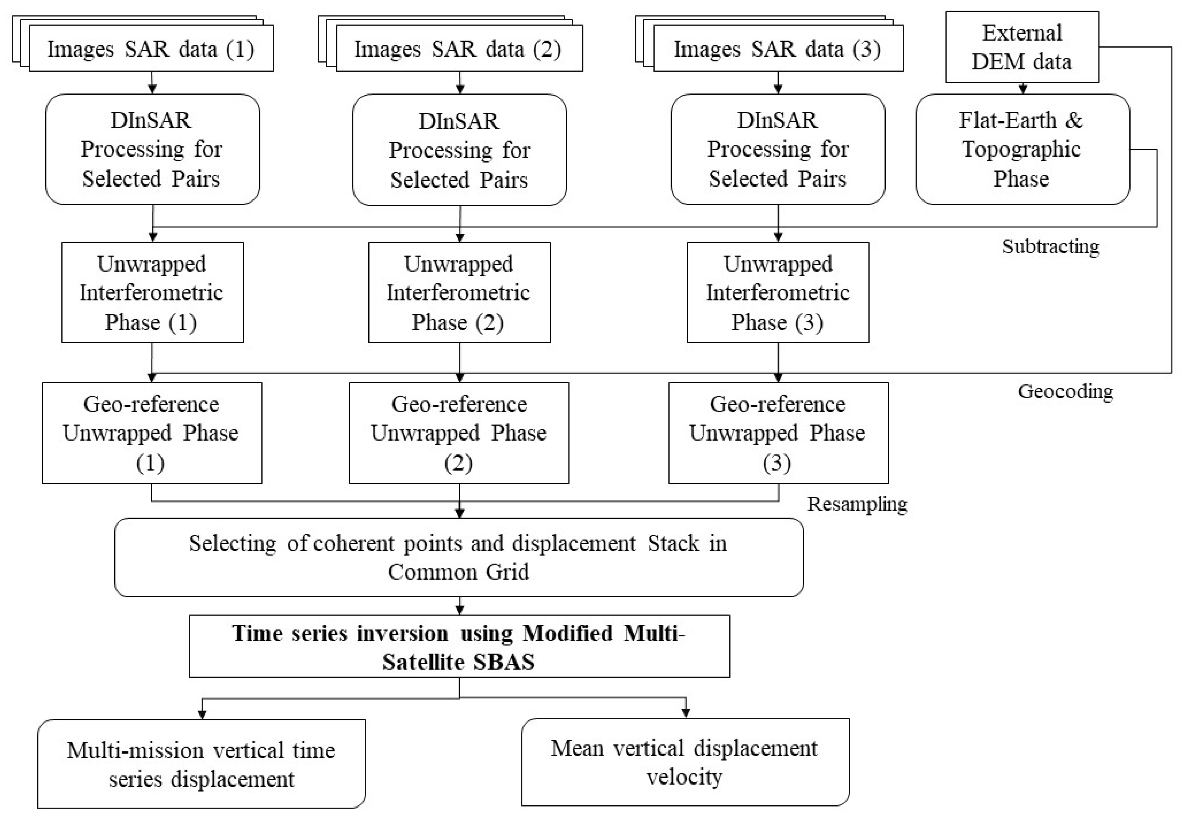
The proposed methodology comprised a three-stage approach to integrate both temporally overlapping and temporally-gapped multi-satellite SAR data. The first stage aimed to process the three SAR data tracks individually. Next, the unwrapped phases were geocoded and resampled at selected high coherent points. Finally, the vertical time series displacement was retrieved based on the Multi-satellite SBAS integration. The method integrated SAR data based on truncated Singular Value Decomposition (TSVD) and least square. The flowchart of the proposed methodology is shown in Figure 2.
2.2.1. Surface Displacement Using Multi-Baseline DInSAR
Multi-baseline DInSAR technique employed the appropriate selection of SAR image pairs satisfying short temporal and spatial baselines. Therefore, temporal and spatial phase decorrelation components were minimized to enhance the phase quality of the processed pixels. Multi-baseline DInSAR processing chain entailed a set of processes for each image pair. Initially, the SAR image pair was co-registered. Next, the phase interferogram was generated. After that, the flat-earth phase, and the topographical phase were eliminated. Then, the multi-looking in the range and azimuth directions was employed to suppress speckle noise and increase the signal-to-noise ratio. Finally, phase filtering and unwrapping. Notably, orbital errors were eliminated based on a linear empirical function whereas atmospheric delays were minimized using atmospheric filtering.
2.2.2. Selection of High Coherent Points
To integrate multi-satellite displacement, it was crucial to retrieve a significant number of high-coherence points. To this target, both PS and DS measurements were fundamentally utilized [45]. In the case of PS, temporal amplitude stability approximated the phase stability based on the Amplitude Dispersion Index where the and were the mean and standard deviation of the amplitudes for a specific pixel, respectively. Initial consideration for PS candidates was given to pixels with . Unlike PS, DS preserved a moderate level of coherence during one or more SAR acquisition periods. The value of complex coherence at a specific pixel in an interferometric pair was calculated as follows:
where L was the number of statistically homogeneous pixels (SHPs) surrounding the central pixel, and represented the complex phase values of the SAR image pair, the coherence magnitude defined the degree of coherence and represents the spatially averaged interferometric phase.
Using statistical similarity tests based on time series amplitudes, such as the Kolmogorov–Smirnov (KS) and Anderson–Darlington (AD) tests, the SHPs for the central pixel can be determined. Initially, DS candidates were chosen from points with average temporal coherence of more than 0.5 and more than 20 SHPs. The spatially averaged phases replaced the original phases of a subset of DS locations. The DS points that correspond with PS points were eliminated to preserve the phases of point-wise PSs. It is worth noting that in every interferogram, PS coherence was always equal to one. The chosen PSs and DSs were then integrated for joint processing in the subsequent analysis. The unwrapped phase was converted into displacements at the high-coherence points in terms of the wavelength as follows:
At each selected high-coherence point, the vertical component of displacement was obtained using Equation (3) based on the incidence angle as follows:
The vertical displacement values resulting from interferograms were geocoded to provide a common grid of high-coherent points on which the multi-satellite SBAS integration step was employed.
2.2.3. Multi-Satellite SBAS Integration
To adapt traditional SBAS for multi-satellite SAR data integration, consider was the number of interferograms formed by multi-satellite SAR images spanning a period from where was the reference starting date. Consequently, the vertical displacement time series was reconstructed according to [15] as follows:
where was similar to an incidence matrix formed using the time intervals between successive SAR images, while was the vector of vertical displacements. Also, represented the unknown vertical velocities time series.
Because this system of equation was under-determined, and in turn, did not admit a unique solution that represents a canonical example of a linear discrete ill-posed problem, replacing the “original” linear system with a nearby system (less sensitive to perturbations of the right-hand side of the system) will provide a meaningful solution for this system [19]. This operation is called regularization which was formed using TSVD [46] as stated in Equation (5), such that be decomposed into three matrices and .
where and are orthogonal, and was a diagonal matrix formed using Equation (6) where r was the rank of .
The main principle of TSVD and standard form regularization was to define a well-posed problem for the ill-posed problem. In the case of TSVD, one approximates the matrix with one of lower rank k and ignores components of the right-hand side corresponding to the ignored components of . The matrix used in TSVD was defined as the rank-k matrix.
where, and equal S with the smallest singular values replaced by zeros. The solution of Equation (4) based on TSVD is defined by:
The matrix is the pseudoinverse of :
According to the TSVD method we obtain with respect to . The TSVD solves the unknown parameters for each pixel, and numerical integration reconstructed the displacement time series from the computed displacement velocities. We also obtained a combined multi-satellite surface displacement time series using this method, which was relevant to the first acquisition date.
2.2.4. Evaluation Criteria
Due to the lack of field measurements, cross-validation was employed to evaluate the integration results. Two consistency assessments were utilized [5,8]. First, the mean vertical displacement velocity from stacking all interferograms (involved in the integration process) was compared to the mean displacement velocity from integration. Reasonable results of this comparison should confirm the consistency between the two maps. The second assessment compares the average displacement velocity from applying the SBAS to each dataset with their time counterparts from integration. This criterion investigated whether the two maps exhibit a similar behavior. Therefore, standard deviations of the differences were computed.
3. Results and Analysis
The experimental design has involved three sets of SAR data as explained in Section 2.1.2. Cross-validation has been employed to assess the validity of the proposed procedure. To the best of our knowledge, the proposed methodology represents a pioneering approach that integrates 20 years of multi-satellite SAR datasets over Almokattam city. To generate the long-term displacement time series, the LOS displacements were calculated for all interferograms within each dataset to generate the long-term displacement time series. It is worth noting that these displacements have been computed at a set of high-coherence points based on a specific threshold. Next, all interferograms have been geocoded to the WGS84 geographic coordinate system. Then, the combined vertical displacement time series for the ENVISAT, ERS, and S1 datasets have been gained using the TSVD inversion. This corresponds to the ERS dataset’s earliest acquisition date of (i.e., the image acquired on 20 January 2000).
3.1. Multi-Baseline DInSAR Displacement
SAR image pairs were chosen based on strict criteria: a perpendicular baseline of less than 500 m for ENVISAT and ERS data, and less than 180 m for Sentinel-1 data. Additionally, all image pairs have a temporal baseline of less than 365 days. Figure 3 presents the distribution of SAR images in the temporal/perpendicular baseline plane, along with connecting lines for the data acquisition points.
Building upon step 1, the DInSAR technique was implemented on the co-registered SAR image pairs by applying a high-resolution 1 arc-second SRTM3 Digital Elevation Model (DEM) to account for topographic phase removal. Additionally, a multi-look was applied for every interferogram (with 1 × 5, and 10 × 2 looks, in the range × azimuth direction for ENVISAT, ERS, and S1, respectively). Then, the noise was filtered from single interferograms using the Goldstein filter [47] while the unwrapped phase was obtained using the statistical-cost network-flow algorithm [48]. After that, a two-dimensional quadratic model was employed to remove baseline residual errors and long-wavelength atmospheric artifacts.
The LOS displacement was then retrieved for high-coherence pixels in each interferogram using a coherence threshold of 0.50. Finally, the geocoded LOS displacements from all interferograms were referenced to the WGS84 system for subsequent analysis. Figure 4a presents the mean vertical displacement velocity from 20 January 2000 to 15 July 2020. This velocity was calculated by stacking the vertical displacements derived from all interferograms used in the analysis. Areas experiencing subsidence (negative velocity) were depicted in shades of red in the western part of the city with a maximum of −5.26 mm/year.
3.2. Multi-Satellite SBAS Displacement
Leveraging the proposed methodology, we successfully integrated temporally overlapped and gapped ENVISAT, ERS, and S1 DInSAR-derived displacement values. This process generated a long-term displacement time series spanning over two decades (2000–2020). Figure 4b presents the mean displacement velocity map for the combined ERS, ENVISAT, and Sentinel-1 data. This map, generated using the set of high-coherence points common across all three datasets, reveals a maximum subsidence velocity of −2.32 mm/year in the western part of the city. As shown in Figure 4, consistent spatial patterns of displacement rates are observed across pre- and post-integration results, validating the proposed method’s efficacy.
3.3. Displacement from Individual Datasets
Mean vertical displacement velocity maps were generated using the SBAS method on the ERS, ENVISAT, and Sentinel-1 datasets, respectively, as shown in Figure 5a,c,e. The displacement velocities derived from each dataset were then compared to their corresponding temporal counterparts obtained from the integration process.
The results from the ERS data (2000–2010) exhibit a wider displacement range (from −59.57 to 19.19 mm/year) compared to both the ENVISAT data (2004–2012; −13.39 to 7.66 mm/year) and Sentinel-1 data (2014–2020; −15.53 to 17.21 mm/year). Despite these variations, a similar overall displacement pattern is evident across all three datasets, as illustrated in Figure 5a,c,e. However, it is important to acknowledge that the different time intervals and image acquisition geometries, including resolution, azimuth, and incidence angle contribute to some discrepancies observed in the displacement rate maps.
Following the generation of the integrated vertical displacement time series from the three datasets, the mean displacement velocity for each dataset’s corresponding period was extracted individually from the combined time series. These extracted velocities are presented in Figure 5b,d,f, respectively. These extracted velocities were then compared to their counterparts computed using the SBAS method. The spatial distribution of displacement for each dataset exhibited minimal variation between the pre-integration and post-integration results, with only insignificant differences in magnitude. This consistency signifies the successful integration achieved by the Multi-Satellite SBAS-based method. The displacement range observed in the ERS and ENVISAT maps exhibits a greater magnitude difference compared to the Sentinel-1 map. This can be attributed to the fewer ERS and ENVISAT interferograms included in the integration process compared to the larger number of Sentinel-1 interferograms.
3.4. Evaluation
The evaluation has adhered to the criteria outlined in Section 2.2.4. First, the pre-integration displacements from all interferograms were compared to their counterparts after integration. Second, the differences between pre and post-integration displacements using interferograms of the individual datasets were compared. The numeric and visualized analysis of results is shown in the upcoming subsections.
3.4.1. Displacement Based on All Interferograms
The statistical analysis signifies the effectiveness of the integration approach, as evidenced by the mean difference of mm with of 2.88 mm/year. Additionally, the correlation coefficients between results were determined. The scatter plot of results is shown in Figure 6a, with a correlation coefficient of 0.97, demonstrating that the two results had a consistent deformation pattern and a high level of agreement. A histogram was established for the displacement differences as shown in Figure 6b.
3.4.2. Displacement from Individual Datasets
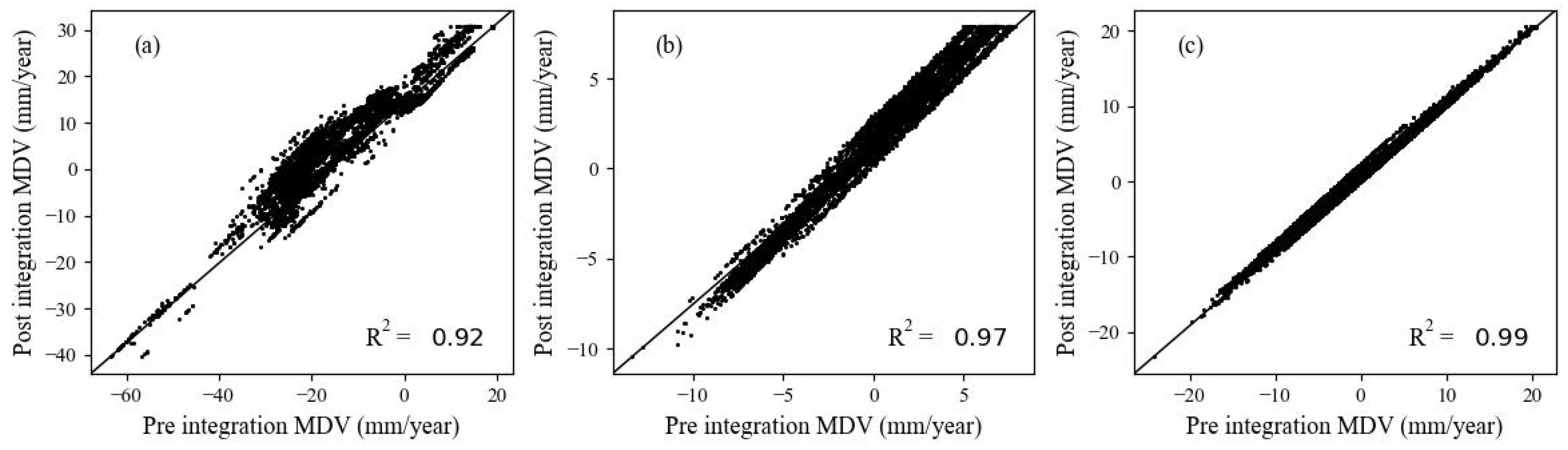
Mean displacement velocities from ENVISAT, ERS, and Sentinel-1 data based on the SBAS method were determined and compared to their counterparts from the proposed method. The differences were summarized in Table 2 with a mean difference of 1.87, 1.5, and 1.04 mm for ERS, ENVISAT, and Sentinel-1 data, respectively. This finding denotes the significance of the proposed method for retrieving the long-term multi-satellite vertical displacement time series. A histogram of differences was established as shown in Figure 7a–c. The differences yielded a median of 1.85, 1.49, and 1.08 mm/year for ERS, ENVISAT, and S1, respectively, indicating that S1-derived displacements were more reasonable than those from ERS and ENVISAT. The correlation coefficients were computed separately for the mean displacement velocity pre and post-integration as presented in Figure 8. It was found that the correlation coefficients for the ERS, ENVISAT, and sentential-1 datasets were 0.92, 0.97, and 0.99, respectively. Such findings demonstrated a highly consistent deformation pattern between the results. The of the ERS, ENVISAT, and sentential-1 datasets were 1.92, 1.66, and 1.19 mm, respectively. Therefore, the proposed integration approach (i.e., Multi-satellite SBAS) is efficient as seen by the cross-validation (i.e., ), particularly the S1 dataset that outperformed ERS and ENVISAT datasets.
4. Discussion
The research methodology proposed Multi-Satellite SBAS to retrieve long-term ground displacement. In this section, several key aspects have been investigated to measure the potential of the proposed method. These aspects encompass the geological characteristics of the study area, Multi-Satellite SBAS, and comparison with previous methods.
4.1. Displacement in Almokattam City, Causes and Implications
The geological composition of Almokattam Mountain has been comprehensively investigated in the literature research. It was reported that the Upper Eocene rocks (Maadi Formation) are composed of brown-colored cracked limestone, marl, and claystone. Also, the Middle Eocene rocks (Almokattam Formation) consist of white to gray limestone with less abundant clay and marl. This structure was reported as one of the major causes of the steep slopes [49]. Therefore, the Almokattam Formation exhibits greater solidity and durability than the Maadi Formation [42]. Small-scale folds sloping downwards in a southeast or east direction were identified. These folds were affiliated with block faulting [50], characterized by a space from 5 to 8 m. Also, they are predominantly steep and characterized by slabs of less than 20 m to 110 m in length, deep corners, and angles between 60 and 70 degrees [51].
The experimental results showed significant subsidence from 2000 to 2010, as shown in Figure 5a. It is worth noting that these findings are consistent with the well-known historical rock failures in 1994, 2004, and 2008. The main causes of the deformation of Almokattam city include (1) the rugged topography ranging from 11 to 220 m; (2) the existence of possible active faults; (3) the heterogeneous nature of the Mountain’s rocks; (4) the environmental issues such as leakage of sewage water; (5) the angle of the slope is proportional to the likelihood of rock failure. The steeper the terrain, the higher the slope angle value. In Almokattam city, where slopes reach 70 degrees, the slope is one of the most critical elements impacting slope stability; (6) the natural ability of the Almokattam mountain ramp is corrosion and instability, and the instability has worsened due to human activity. The deterioration of the situation observed in recent decades was likely attributed to the increasing population as shown in Figure 1b,c,d which increased water infiltration, as well as unregulated building construction; (7) the removal and replacement of vegetation in the built-up region.
Figure 4b, illustrates irregular deformation at several locations. The most vulnerable place to landslides was the western part of Almokattam city where the displacement value reached −2.32 mm/year. This is also in line with the continuous disastrous subsidence at the western part Almokattam Plateau that occurred during the period of study. The validation results demonstrated that the proposed method has potentially provided valuable subsidence information.
4.2. Multi-Satellite SBAS for SAR Data Integration
InSAR has proven to be one of the most powerful techniques for monitoring ground subsidence. However, a single sensor and single platform InSAR analysis face particular obstacles in the urban setting. Therefore, leveraging the increasing availability of SAR satellites with diverse temporal and spatial resolutions was sought to derive a multi-platform InSAR time series. Such integration is anticipated to mitigate the limitations of single-sensor or single-platform data. This was the inspiration for our post-processing integration method. Additionally, the characteristics of the proposed method compared to literature research include: (1) no external deformation model is required to link the time-gaped data; (2) LOS ground displacement is generated independently of a pre-definition of a displacement model; (3) a relatively small number of SAR scenes are utilized; (4) Exploiting the advantages of both PS and DS to increase the density of high-coherence points.
4.3. Comparison with Previous Studies
The field measurements were not available to perform evaluation and cross-validation was employed. Consequently, the major research findings were compared to the previous research in the study area. Two literature research were involved [52,53] because their investigations utilized InSAR data within our study period. Poscolieri et al. [52] detected ground deformation in the Greater Cairo Metropolitan Region from 2003 to 2009 using ASAR Single Look Complex VV-polarization scenes in descending mode. They employed Interferometric Stacking and Persistent Scatterers Interferometry to retrieve the displacement. They have reported a subsidence rate of −2 to −5 mm/year in the west and −5 to −7 mm/year in the west-south areas of the city. In addition, numerous normal faults have been mapped with an NW-SE direction [51]. They also demonstrated a sinking phenomenon between these structures, particularly at the point targets located on the down-thrown side of the normal faults.
Further, Aly et al. [53] utilized a permanent scatterer interferometric technique to quantify Greater Cairo’s subsidence with its spatial and temporal variability. The dataset comprised 34 InSAR images from the ERS-1 and ERS-2 from 1993 to 2000. The largest subsidence was reported for the west side of Almokattam Hill with a rate of −4 to −7 mm/year. Then, this rate continued to drop progressively to the middle of the hill by −1 to −3 mm/year. In addition, certain uplifts were recorded in various places of the hill particularly in the east. Lastly, they highlighted insignificant differences in vertical displacement between their findings and previous research within the study area. They attributed such differences to diverse methodologies, SAR datasets, and time intervals.
Compared to the aforementioned, our proposed methodology has achieved sub-millimeter accuracy in estimating both subsidence and its trend. Sentinel-1 results outperformed those from ENVISAT and ERS. With a few minor exceptions, the results were generally consistent. Sentinel-1 results exhibited a high degree of consistency. On the other hand, the findings from the other datasets which encompassed the earliest time frames displayed the lowest correlations. This could be attributed to the larger number and small temporal resolution of Sentinel-1 images that were utilized in the integration process compared to ENVISAT and ERS images. Sentinel-1’s data were highly consistent, which promotes our hypothesis that vertical displacement accounts for the majority of the displacement. Finally, our study demonstrated the significance of integrating multi-sensor and multi-track SAR data to retrieve long-term displacement. Further, the integration of InSAR data from multiple satellites and tracks optimizes the potential of these datasets, such as the comprehensive coverage for deformation monitoring.
5. Conclusions
This paper introduced multi-satellite DInSAR data integration based on TSVD. The developed method integrated both temporal-overlapped and temporal-gaped systems of vertical displacement time series. The experiments were conducted using 20 years of SAR data from Almokattam City in Egypt. According to the cross-validation, the integration allowed for a better interpretation of the deformation behavior within the study area. It is believed that the integration results are anticipated to support the decision-making authorities for risk mitigation and sustainability. It can be concluded that the proposed method has a potential performance on multi-satellite DInSAR integration, however, it should be assessed, adjusted, and validated by extra types of measurements (GPS, leveling, etc). An essential outlook of this research is to extend the Multi-Satellite SBAS to combine DInSAR-driven 3D displacement time series. Such an extension is subject to the validity of some additional ground deformation signal constraints, and the accessibility of SAR ascending/descending flight passes over the same scene on Earth.
Author Contributions
Conceptualization, D.A. and X.-L.D.; methodology, D.A.; software, D.A.; validation, D.A., X.-L.D. and R.F.; formal analysis, D.A; investigation, D.A.; resources, X.-L.D.; data curation, D.A.; writing—original draft preparation, D.A.; writing—review and editing, D.A.; visualization, D.A.; supervision, D.A.; project administration, D.A.; funding acquisition, D.A. All authors have read and agreed to the published version of the manuscript.
Funding
This research received no external funding.
Data Availability Statement
The data presented in this study are available on request from the corresponding author.
Conflicts of Interest
All authors declare that there are no conflicts of interest.
References
- Aboushook, M.; EL-Sohby, M.; Mazen, O. Slope degradation and analysis of Mokattam plateau, Egypt. In Proceedings of the 2nd International Conference on Geotechnical Site Characterization (ISC-2), Porto, Portugal, 19–22 September 2004; pp. 1081–1887. [Google Scholar]
- Aimaiti, Y.; Yamazaki, F.; Liu, W. Multi-Sensor InSAR Analysis of Progressive Land Subsidence over the Coastal City of Urayasu, Japan. Remote Sens. 2018, 10, 1304. [Google Scholar] [CrossRef]
- Luo, Q.; Perissin, D.; Lin, H.; Li, Q.; Duering, R. Railway subsidence monitoring by high-resolution INSAR time series analysis in Tianjin. In Proceedings of the 2011 19th International Conference on Geoinformatics, Shanghai, China, 24–26 June 2011; pp. 1–4. [Google Scholar] [CrossRef]
- Sun, Q.; Hu, J.; Zhang, L.; Ding, X. Towards Slow-Moving Landslide Monitoring by Integrating Multi-Sensor InSAR Time Series Datasets: The Zhouqu Case Study, China. Remote Sens. 2016, 8, 908. [Google Scholar] [CrossRef]
- Wang, L.; Marzahn, P.; Bernier, M.; Ludwig, R. Sentinel-1 InSAR measurements of deformation over discontinuous permafrost terrain, Northern Quebec, Canada. Remote Sens. Environ. 2020, 248, 111965. [Google Scholar] [CrossRef]
- Ren, H.; Feng, X. Calculating vertical deformation using a single InSAR pair based on singular value decomposition in mining areas. Int. J. Appl. Earth Obs. Geoinf. 2020, 92, 102115. [Google Scholar] [CrossRef]
- Peng, M.; Zhao, C.; Zhang, Q.; Lu, Z.; Bai, L.; Bai, W. Multi-Scale and Multi-Dimensional Time Series InSAR Characterizing of Surface Deformation over Shandong Peninsula, China. Appl. Sci. 2020, 10, 2294. [Google Scholar] [CrossRef]
- Pawluszek-Filipiak, K.; Borkowski, A. Integration of DInSAR and SBAS Techniques to Determine Mining-Related Deformations Using Sentinel-1 Data: The Case Study of Rydułtowy Mine in Poland. Remote Sens. 2020, 12, 242. [Google Scholar] [CrossRef]
- Hooper, A.; Bekaert, D.; Spaans, K.; Arıkan, M. Recent advances in SAR interferometry time series analysis for measuring crustal deformation. Tectonophysics 2012, 514–517, 1–13. [Google Scholar] [CrossRef]
- Ferretti, A.; Prati, C.; Rocca, F. Permanent scatterers in SAR interferometry. IEEE Trans. Geosci. Remote Sens. 2001, 39, 8–20. [Google Scholar] [CrossRef]
- Ferretti, A.; Prati, C.; Rocca, F. Nonlinear subsidence rate estimation using permanent scatterers in differential SAR interferometry. IEEE Trans. Geosci. Remote Sens. 2000, 38, 2202–2212. [Google Scholar] [CrossRef]
- Hooper, A.; Zebker, H.; Segall, P.; Kampes, B. A new method for measuring deformation on volcanoes and other natural terrains using InSAR persistent scatterers. Geophys. Res. Lett. 2004, 31. [Google Scholar] [CrossRef]
- Werner, C.L.; Wegmüller, U.; Strozzi, T.; Wiesmann, A. Interferometric point target analysis for deformation mapping. In Proceedings of the IGARSS 2003. 2003 IEEE International Geoscience and Remote Sensing Symposium. Proceedings (IEEE Cat. No.03CH37477), Toulouse, France, 21–25 July 2003; Volume 7, pp. 4362–4364. [Google Scholar]
- Kampes, B.M. Radar Interferometry; Springer: Berlin/Heidelberg, Germany, 2006; Volume 12. [Google Scholar]
- Berardino, P.; Fornaro, G.; Lanari, R.; Sansosti, E. A new algorithm for surface deformation monitoring based on small baseline differential SAR interferograms. IEEE Trans. Geosci. Remote Sens. 2002, 40, 2375–2383. [Google Scholar] [CrossRef]
- Mora, O.; Mallorqui, J.; Broquetas, A. Linear and nonlinear terrain deformation maps from a reduced set of interferometric SAR images. IEEE Trans. Geosci. Remote Sens. 2003, 41, 2243–2253. [Google Scholar] [CrossRef]
- Crosetto, M.; Crippa, B. State of the art of land deformation monitoring using differential SAR interferometry. In Proceedings of the ISPRS Hann, ISPRS Hannover Workshop 2005, Hannover, Germany, 17–20 May 2005. [Google Scholar]
- Fornaro, G.; Pauciullo, A.; Serafino, F. Deformation monitoring over large areas with multipass differential SAR interferometry: A new approach based on the use of spatial differences. Int. J. Remote Sens. 2009, 30, 1455–1478. [Google Scholar] [CrossRef]
- Pepe, A.; Solaro, G.; Calò, F.; Dema, C. A Minimum Acceleration Approach for the Retrieval of Multiplatform InSAR Deformation Time Series. IEEE J. Sel. Top. Appl. Earth Obs. Remote Sens. 2016, 9, 3883–3898. [Google Scholar] [CrossRef]
- Zhao, Q.; Ma, G.; Wang, Q.; Yang, T.; Liu, M.; Gao, W.; Falabella, F.; Mastro, P.; Pepe, A. Generation of long-term InSAR ground displacement time-series through a novel multi-sensor data merging technique: The case study of the Shanghai coastal area. ISPRS J. Photogramm. Remote Sens. 2019, 154, 10–27. [Google Scholar] [CrossRef]
- Gray, L. Using multiple RADARSAT InSAR pairs to estimate a full three-dimensional solution for glacial ice movement. Geophys. Res. Lett. 2011, 38. [Google Scholar] [CrossRef]
- Gudmundsson, S.; Sigmundsson, F.; Carstensen, J.M. Three-dimensional surface motion maps estimated from combined interferometric synthetic aperture radar and GPS data. J. Geophys. Res. Solid Earth 2002, 107, ETG 13-1–ETG 13-14. [Google Scholar] [CrossRef]
- Hu, J.; Ding, X.L.; Li, Z.W.; Zhu, J.J.; Sun, Q.; Zhang, L.; Omura, M. A kalman filter based mtinsar methodology for derving 3d surface displacement evolutions. North 2012, 2011, 19–23. [Google Scholar]
- Lu, J. Sentinel-1 Toolbox Offset Tracking Tutorial; ESA: Montreal, QC, Canada, 2016. [Google Scholar]
- Wright, T.J.; Parsons, B.E.; Lu, Z. Toward mapping surface deformation in three dimensions using InSAR. Geophys. Res. Lett. 2004, 31. [Google Scholar] [CrossRef]
- Saraswat, A.; Tsai, Y.L.S.; Chen, F.C.; Han, J.Y. 3d Deformation Analysis in a Metropolitan Area During Ongoing Subway Construction Using Time Series Insar. Preprint. 2024. Available online: https://ssrn.com/abstract=4726193 (accessed on 21 April 2024).
- Jo, M.J.; Jung, H.S.; Won, J.S.; Poland, M.P.; Miklius, A.; Lu, Z. Measurement of slow-moving along-track displacement from an efficient multiple-aperture SAR interferometry (MAI) stacking. J. Geod. 2015, 89, 411–425. [Google Scholar] [CrossRef]
- Jung, H.S.; Won, J.S.; Kim, S.W. An Improvement of the Performance of Multiple-Aperture SAR Interferometry (MAI). IEEE Trans. Geosci. Remote Sens. 2009, 47, 2859–2869. [Google Scholar] [CrossRef]
- Fialko, Y.; Sandwell, D.; Simons, M.; Rosen, P. Three-dimensional deformation caused by the Bam, Iran, earthquake and the origin of shallow slip deficit. Nature 2005, 435, 295–299. [Google Scholar] [CrossRef] [PubMed]
- Fialko, Y.; Simons, M.; Agnew, D. The complete (3-D) surface displacement field in the epicentral area of the 1999 MW7.1 Hector Mine Earthquake, California, from space geodetic observations. Geophys. Res. Lett. 2001, 28, 3063–3066. [Google Scholar] [CrossRef]
- Samsonov, S.; Tiampo, K.F.; Gonzalez, P.; Prieto, J.F.; Camacho, A.G.; Fernández, J. Surface deformation studies of Tenerife Island, Spain from joint GPS-DInSAR observations. In Proceedings of the 2008 Second Workshop on Use of Remote Sensing Techniques for Monitoring Volcanoes and Seismogenic Areas, Napoli, Italy, 11–14 November 2008; pp. 1–6. [Google Scholar]
- Chen, M.; Xu, G.; Zhang, T.; Xie, X.; Chen, Z. A novel method for inverting coseismic 3D surface deformation using InSAR considering the weight influence of the spatial distribution of GNSS points. Adv. Space Res. 2024, 73, 585–596. [Google Scholar] [CrossRef]
- Joughin, I.; Kwok, R.; Fahnestock, M. Interferometric estimation of three-dimensional ice-flow using ascending and descending passes. IEEE Trans. Geosci. Remote Sens. 1998, 36, 25–37. [Google Scholar] [CrossRef]
- Samsonov, S. Three-dimensional deformation time series of glacier motion from multiple-aperture DInSAR observation. J. Geod. 2019, 93, 2651–2660. [Google Scholar] [CrossRef]
- Yang, Z.; Li, Z.; Zhu, J.; Yi, H.; Hu, J.; Feng, G. Deriving Dynamic Subsidence of Coal Mining Areas Using InSAR and Logistic Model. Remote Sens. 2017, 9, 125. [Google Scholar] [CrossRef]
- Casu, F.; Manconi, A.; Pepe, A.; Lanari, R. Deformation Time-Series Generation in Areas Characterized by Large Displacement Dynamics: The SAR Amplitude Pixel-Offset SBAS Technique. IEEE Trans. Geosci. Remote Sens. 2011, 49, 2752–2763. [Google Scholar] [CrossRef]
- Samsonov, S.; d’Oreye, N. Multidimensional time-series analysis of ground deformation from multiple InSAR data sets applied to Virunga Volcanic Province. Geophys. J. Int. 2012, 191, 1095–1108. [Google Scholar] [CrossRef]
- Pepe, A.; Solaro, G.; Dema, C. A Minimum Curvature Combination Method for the Generation of Multi-Platform DInSAR Deformation Time-Series. In Proceedings of the FRINGE 2015: Advances in the Science and Applications of SAR Interferometry and Sentinel-1 InSAR Workshop, Frascati, Italy, 23–27 March 2015; Ouwehand, L., Ed.; ESA: Frascati, Italy, 2015; Volume 731, p. 9. [Google Scholar]
- Samsonov, S.V.; Blais-Stevens, A. Estimating volume of large slow-moving deep-seated landslides in northern Canada from DInSAR-derived 2D and constrained 3D deformation rates. Remote Sens. Environ. 2024, 305, 114049. [Google Scholar] [CrossRef]
- Tao, Q.; Zheng, Z.; Zhai, M.; Zhang, S.; Hu, L.; Liu, T. Sensitivity and reliability analysis to MSBAS regularization for the estimation of surface deformation over a mine. Geocarto Int. 2024, 39, 2329669. [Google Scholar] [CrossRef]
- Tang, W.; Gong, Z.; Sun, X.; Liu, Y.; Motagh, M.; Li, Z.; Li, J.; Malinowska, A.; Jiang, J.; Wei, L.; et al. Three-dimensional surface deformation from multi-track InSAR and oil reservoir characterization: A case study in the Liaohe Oilfield, northeast China. Int. J. Rock Mech. Min. Sci. 2024, 174, 105637. [Google Scholar] [CrossRef]
- Kamel, A.; El Sokkary, A. Geologic hazards assessment of Cairo and vicinity. Nat. Hazards 1996, 13, 253–274. [Google Scholar] [CrossRef]
- Cuvillier, J. Revision du Nummulitique Egyptein; MWRI Central Library: Cairo, Egypt, 1930. [Google Scholar]
- Cuvillier, J. A conglomerate in the nummulitic formation of Gebel Moqattam, near Cairo. Geol. Mag. 1927, 64, 522–523. [Google Scholar] [CrossRef]
- Liang, H.; Li, X.; Zhang, L.; Chen, R.F.; Ding, X.; Chen, K.L.; Wang, C.S.; Chang, C.S.; Chi, C.Y. Investigation of Slow-Moving Artificial Slope Failure with Multi-Temporal InSAR by Combining Persistent and Distributed Scatterers: A Case Study in Northern Taiwan. Remote Sens. 2020, 12, 2403. [Google Scholar] [CrossRef]
- Hansen, P.C. The truncatedSVD as a method for regularization. BIT Numer. Math. 1987, 27, 534–553. [Google Scholar] [CrossRef]
- Goldstein, R.; Werner, C. Radar interferogram filtering for geophysical applications. Geophys. Res. Lett. 1998, 25, 4035–4038. [Google Scholar] [CrossRef]
- Chen, C.; Zebker, H. Phase unwrapping for large SAR interferograms: Statistical segmentation and generalized network models. IEEE Trans. Geosci. Remote Sens. 2002, 40, 1709–1719. [Google Scholar] [CrossRef]
- von Zittel, K.A. Beitraege zur Geologie und Palaeontologie der libyschen Wüste und der Angrenzenden Gebiete von Aegypten I Theil; Fischer, T., Ed.; Hansebooks: Norderstedt, Germany, 1883. [Google Scholar]
- El Shazly, E.; Hady, M.A.; Salman, A.; El Rakaiby, M.; Morsy, M.; El Aassy, I.; El Shazly, M. Geological Investigations on Gebel El Mokattam Area; Remote Sensing Center: Cairo, Egypt, 1976; Volume 23. [Google Scholar]
- Moustafa, A.; El-Nahhas, F.; Tawab, S.A. Engineering geology of Mokattam city and vicinity, eastern Greater Cairo, Egypt. Eng. Geol. 1991, 31, 327–344. [Google Scholar] [CrossRef]
- Poscolieri, M.; Parcharidis, I.; Foumelis, M.; Rafanelli, C. Ground Deformation Monitoring in the Greater Cairo Metropolitan Region (Egypt) by SAR Interferometry. Environ. Semeiot. 2011, 4, 17–45. [Google Scholar] [CrossRef]
- Aly, M.H.; Zebker, H.A.; Giardino, J.R.; Klein, A.G. Permanent Scatterer investigation of land subsidence in Greater Cairo, Egypt. Geophys. J. Int. 2009, 178, 1238–1245. [Google Scholar] [CrossRef]
Figure 1.
Study area and data distribution. (a) Location of the Almokattam city on Egypt map. (b) SAR data distribution. (c–e): Urban growth from 2000 to 2017.
Figure 1.
Study area and data distribution. (a) Location of the Almokattam city on Egypt map. (b) SAR data distribution. (c–e): Urban growth from 2000 to 2017.

Figure 2.
Research workflow.

Figure 3.
Distribution of SAR data in the temporal and perpendicular baseline domain. (a) ERS. (b) ENVISAT. (c) sentinel-1.
Figure 3.
Distribution of SAR data in the temporal and perpendicular baseline domain. (a) ERS. (b) ENVISAT. (c) sentinel-1.

Figure 4.
Mean displacement velocity map. (a) Pre-integration (b) Post integration.

Figure 5.
Mean displacement velocity map. ERS (20 January 2000 to 17 February 2005), ENVISAT (13 May 2004 to 6 March 2012), and Sentinel-1 (9 October 2014 to 15 July 2020). (a,c,e): mean displacement pre-integration. (b,d,f): mean displacement pre-integration.
Figure 5.
Mean displacement velocity map. ERS (20 January 2000 to 17 February 2005), ENVISAT (13 May 2004 to 6 March 2012), and Sentinel-1 (9 October 2014 to 15 July 2020). (a,c,e): mean displacement pre-integration. (b,d,f): mean displacement pre-integration.

Figure 6.
Scatterplot and comparison of mean displacement velocity at high-coherence points pre and post-integration. (a) Correlation between mean displacement velocity pre- and post-integration. (b) Histogram of differences between mean displacement velocity pre- and post-integration.
Figure 6.
Scatterplot and comparison of mean displacement velocity at high-coherence points pre and post-integration. (a) Correlation between mean displacement velocity pre- and post-integration. (b) Histogram of differences between mean displacement velocity pre- and post-integration.

Figure 7.
Histograms of the displacement differences. (a) ERS. (b) ENVISAT. (c) Sentinel-1.

Figure 8.
Scatterplots of the mean displacement velocities using the SBAS method at high-coherence points. (a) ERS. (b) ENVISAT. (c) Sentinel-1.
Figure 8.
Scatterplots of the mean displacement velocities using the SBAS method at high-coherence points. (a) ERS. (b) ENVISAT. (c) Sentinel-1.


Table 1.
SAR dataset.
| Satellite | ENVISAT | ERS | Sentinel-1 | |||
|---|---|---|---|---|---|---|
| Orbit | Ascending | Descending | Ascending | Descending | Ascending | Descending |
| Period | 21 March 2008–16 March 2009 | 13 May 2004–06 March 2012 | 09 February 2009–27 September 2010 | 20 January 2000–17 February 2005 | 9 October 2014–15 July 2020 | 30 September 2016–29 June 2020 |
| No. of images | 3 | 22 | 4 | 23 | 21 | 17 |
Table 2.
Differences between the mean displacement velocity values of each dataset before and after integration (mm/year).
Table 2.
Differences between the mean displacement velocity values of each dataset before and after integration (mm/year).
| Satellite | ERS | ENVISAT | Sentinel-1 |
|---|---|---|---|
| Min. Difference | 0.97 | 0.002 | 0.0003 |
| Max. Difference | 3.11 | 3.02 | 2.5 |
| Mean. Difference | 1.87 | 1.5 | 1.04 |
| 1.92 | 1.66 | 1.19 | |
| STD | 0.42 | 0.72 | 0.57 |
Disclaimer/Publisher’s Note: The statements, opinions and data contained in all publications are solely those of the individual author(s) and contributor(s) and not of MDPI and/or the editor(s). MDPI and/or the editor(s) disclaim responsibility for any injury to people or property resulting from any ideas, methods, instructions or products referred to in the content. |
© 2024 by the authors. Licensee MDPI, Basel, Switzerland. This article is an open access article distributed under the terms and conditions of the Creative Commons Attribution (CC BY) license (https://creativecommons.org/licenses/by/4.0/).
Share and Cite
MDPI and ACS Style
Amr, D.; Ding, X.-L.; Fekry, R. A Multi-Satellite SBAS for Retrieving Long-Term Ground Displacement Time Series. Remote Sens. 2024, 16, 1520. https://0-doi-org.brum.beds.ac.uk/10.3390/rs16091520
AMA Style
Amr D, Ding X-L, Fekry R. A Multi-Satellite SBAS for Retrieving Long-Term Ground Displacement Time Series. Remote Sensing. 2024; 16(9):1520. https://0-doi-org.brum.beds.ac.uk/10.3390/rs16091520
Chicago/Turabian StyleAmr, Doha, Xiao-Li Ding, and Reda Fekry. 2024. "A Multi-Satellite SBAS for Retrieving Long-Term Ground Displacement Time Series" Remote Sensing 16, no. 9: 1520. https://0-doi-org.brum.beds.ac.uk/10.3390/rs16091520
Note that from the first issue of 2016, this journal uses article numbers instead of page numbers. See further details here.