Article

Remote Sensing and Machine Learning for Accurate Fire Severity Mapping in Northern Algeria

1
Yale Institute for Biospheric Studies, Yale University, 170 Whitney Avenue, RM 213A, New Haven, CT 06511, USA
2
Computer Science Department, Yale University, A.K. Watson Hall, 51 Prospect Street, New Haven, CT 06511, USA
3
Software Engineering Department, ETSI Informatics and Telecommunication, University of Granada, 18071 Granada, Spain
4
Yale Center for Earth Observation, Yale School of the Environment, Yale University, New Haven, CT 06520, USA
5
Yale Peabody Museum, 170 Whitney Ave., New Haven, CT 06511, USA
6
Laboratory of Analysis and Modeling of Random Phenomena (LAMPA), Mouloud Maameri Tizi Ouzou University, BP 17 RP, Tizi-Ouzou 15000, Algeria
*
Author to whom correspondence should be addressed.
Submission received: 22 February 2024 / Revised: 12 April 2024 / Accepted: 22 April 2024 / Published: 25 April 2024
(This article belongs to the Topic Application of Remote Sensing in Forest Fire)

Abstract

:
Forest fires pose a significant threat worldwide, with Algeria being no exception. In 2020 alone, Algeria witnessed devastating forest fires, affecting over 16,000 hectares of land, a phenomenon largely attributed to the impacts of climate change. Understanding the severity of these fires is crucial for effective management and mitigation efforts. This study focuses on the Akfadou forest and its surrounding areas in Algeria, aiming to develop a robust method for mapping fire severity. We employed a comprehensive approach that integrates satellite imagery analysis, machine learning techniques, and geographic information systems (GIS) to assess fire severity. By evaluating various remote sensing attributes from the Sentinel-2 and Planetscope satellites, we compared different methodologies for fire severity classification. Specifically, we examined the effectiveness of reflectance indices-based metrics such as Relative Burn Ratio (RBR) and Difference Burned Area Index for Sentinel-2 (dBIAS2), alongside machine learning algorithms including Support Vector Machines (SVM) and Convolutional Neural Networks (CNN), implemented in ArcGIS Pro 3.1.0. Our analysis revealed promising results, particularly in identifying high-severity fire areas. By comparing the output of our methods with ground truth data, we demonstrated the robust performance of our approach, with both SVM and CNN achieving accuracy scores exceeding 0.84. An innovative aspect of our study involved semi-automating the process of training sample labeling using spectral indices rasters and masks. This approach optimizes raster selection for distinct fire severity classes, ensuring accuracy and efficiency in classification. This research contributes to the broader understanding of forest fire dynamics and provides valuable insights for fire management and environmental monitoring efforts in Algeria and similar regions. By accurately mapping fire severity, we can better assess the impacts of climate change and land use changes, facilitating proactive measures to mitigate future fire incidents.

1. Introduction

Wildfires pose a significant global threat to biodiversity and ecosystem health, particularly impacting diverse plant species vulnerable to recurrent outbreaks [1]. Understanding wildfire severity is crucial for assessing both immediate impacts, such as post-fire organic matter loss, as noted by Gibson et al. [2], and broader ecological and environmental consequences. It is essential to differentiate between fire severity, indicating the intensity of the fire and its landscape effects, and burn severity, which measures the extent of damage to vegetation and soil [3]. Accurate mapping of fire severity not only aids in effective fire management, but also sheds light on global climate change impacts and potential fuel risks, playing a vital role in assessing post-fire vegetation recovery and monitoring species diversity [4]. In this work, we compare computational methods for mapping fire severity using remote sensing data. Our comparison is performed using data from an Algerian forest in the Mediterranean region.
Remote sensing has emerged as a cost-effective and high-resolution alternative to conventional methods for mapping fire severity across diverse landscapes [5]. Despite the wealth of satellite imagery, creating clear and comprehensive maps through classification techniques is imperative. Classification distills complex satellite data into interpretable maps, facilitating better visualization, understanding of wildfire impact, and aiding decision-making processes [6].
Reflectance-based methods utilizing spectral satellite data, including differenced Normalized Burn Ratio (dNBR), Burned Area Index (BAI), and normalized difference vegetation index (NDVI), are widely employed for fire severity mapping [7,8,9,10,11,12]. Research demonstrates that combining indices enhances accuracy in fire severity mapping [13,14]. Various machine learning (ML) approaches, such as Random Forest (RF) and Support Vector Machines (SVM), have been utilized to combine indices, with Lasaponara et al. [13] proposing an innovative approach employing a Self-Organized Map (SOM) with multiple indices, surpassing the performance of methods using fixed thresholds on individual indices. Their unsupervised ML classification method strongly correlates with satellite-based fire severity. SVM and RF methods have shown enhanced performance compared to single-index methods [15,16,17].
Newer ML techniques, notably Convolutional Neural Networks (CNN) [18], have gained significant attention in remote sensing, offering precise fire severity mapping outcomes [19,20,21]. Zhang et al. [22] proposed a CNN-based approach for Forest Fire Susceptibility Modeling using the AlexNet model, demonstrating superior performance compared to RF, SVM, and Kernel logistic regression.
The Mediterranean region in particular faces substantial fire risks due to its dry climate, flammable vegetation, and human activities [23,24]. Annually, over 55,000 fires occur in the at-risk Mediterranean areas, leading to ecological, economic damage, and loss of life “https://effis.jrc.ec.europa.eu (accessed on 9 August 2022)”. In Algeria, despite forests covering only about 0.9% of Algeria’s territory, an average of 1637 fires annually destroyed 35,025 hectares of natural forest between 1985 and 2010 [25,26]. Recent years have seen escalated damage, with over 28,000 hectares consumed from 2012 to 2020 and approximately 45,000 hectares in 2021 alone.
Recent research has begun to address forest fire risks in Algeria, particularly focusing on the northern regions. Studies have explored the utilization of remote sensing data and basic spectral indices such as NDVI and the Combustibility Index for mapping fire risk areas. While the body of work in this area may not be extensive, research conducted by various scholars [27,28,29,30] has provided valuable insights into understanding the spatial distribution of fire risks. These efforts aim to enhance preparedness and response strategies, albeit within the context of limited existing research.
Our work is motivated by the need for a comprehensive study of the region, covering varied terrain characteristics and key parameters. We sought to provide a comprehensive analysis of the region’s diverse terrain and key parameters. We focused on the Akefadou Forest, which lies in the Bejaia and Tizi Ouzou provinces. The area faced recurrent fires from 2012 to 2019 and particularly devastating fires in 2021 and 2023. In this work, we contribute to this global effort by examining the use of spectral indices and machine learning techniques applied to satellite data to map severity in a study area encompassing the Akfadou forest and its surroundings in northern Algeria, where diverse plant species are particularly vulnerable to recurrent wildfires. We conducted a comparative analysis of two spectral parameters, the Relativized Burn Ratio (RBR) and the Difference from Burned Reference Index (dBIAS), alongside two machine learning methods: CNN and SVM.
A disadvantage of supervised ML techniques is that they require data for the training models [21]. The manual labeling of such training data can be labor-intensive and prone to inaccuracies, particularly when accurate details are essential. To enhance the accuracy of machine learning, we propose an innovative approach that semi-automates the labeling of the critical training samples using spectral index data and information from the source dataset. Our proposed method allows for the creation of a more effective Regions of Interest (ROIs) for training sample selection from selected spectral index rasters. By improving both the model’s efficiency and its classifier effectiveness, this approach aims to ensure precise and reliable classification outcomes.
As the basis for mapping fire severity, we utilized satellite data from Sentinel-2 and Planetscope. These satellite systems offer complementary advantages for our analysis. Sentinel-2 provides high-resolution imagery with a wide spectral range, enabling detailed land cover analysis and precise fire severity mapping. On the other hand, Planetscope’s high spatial resolution enhances our ability to capture fine-scale features in the landscape.
Our study presents three major results: (1) We present a comparison of the classifications produced by methods derived from spectral indices and by two ML methods. By applying a more holistic approach, the ML methods achieve better results with respect to a ground truth classification. (2) We introduce a novel semi-automated approach for labeling training data for ML to replace error-prone manual labeling techniques. By creating labeled areas with more complex but accurate boundaries, the new labeling techniques improve the ML results even further with respect to ground truth. (3) We illustrate fire severity classification for areas such as northern Algeria, where typically only satellite and sparse reliable ground truth data can be obtained.

2. Materials and Methods
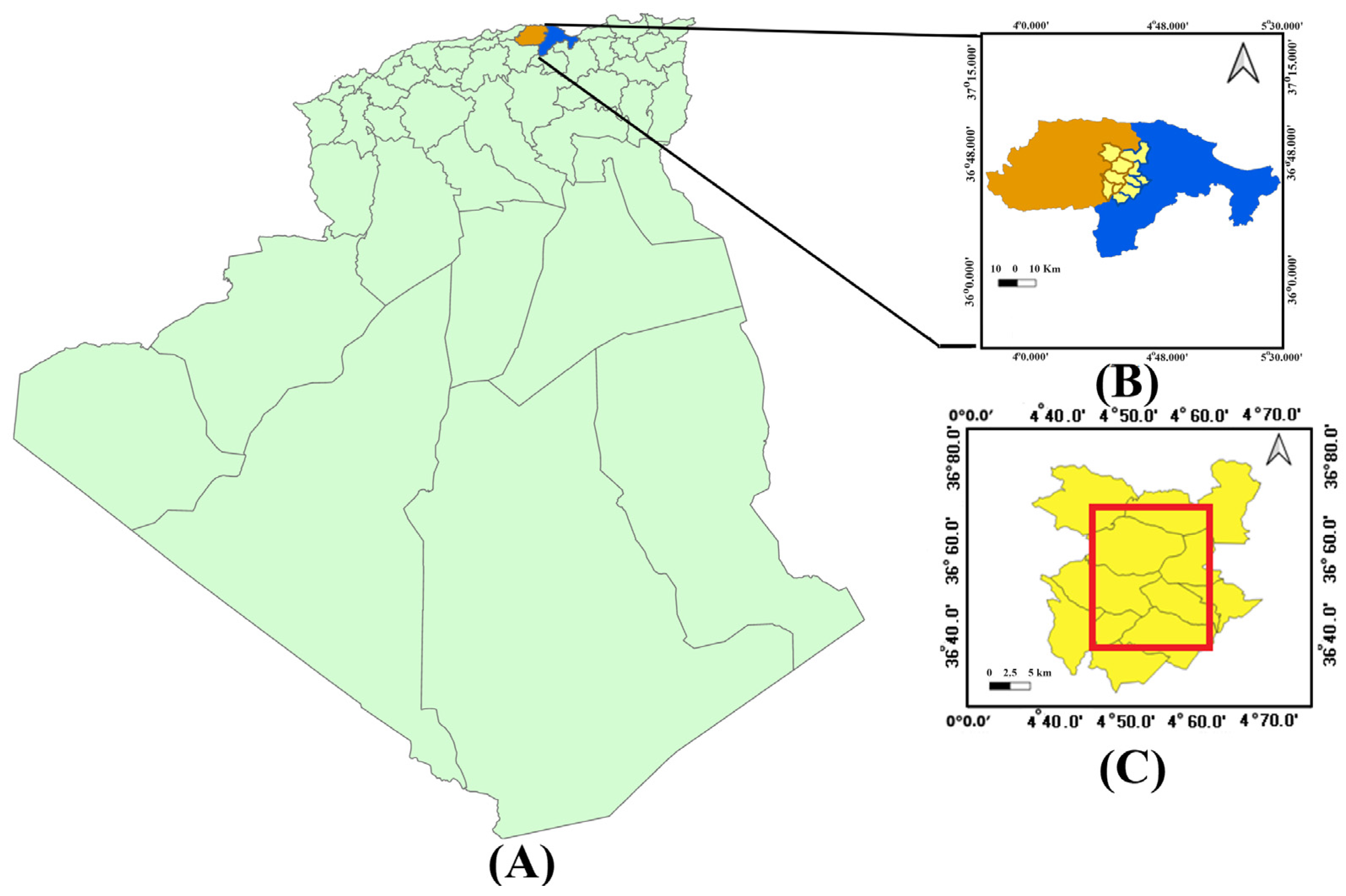
2.1. Study Area

The selected study area covered northern Algeria, comprising the latitudes from 36.52° to 36.73° and longitudes from 4.47° to 4.63°. This region was chosen due to its historical incidence of fires, particularly in Béjaïa, Bouira, Blida, and Tizi Ouzou wilayas. Tizi Ouzou, especially, has been heavily affected by forest fires, ranking among the most impacted provinces over the past decade. We used the DIVA-GIS website “https://www.diva-gis.org/download (accessed on 15 August 2022)” to download the spatial data corresponding to Algeria, and QGIS 3.16 was used to display the shapefile map of this region (Figure 1). The study area comprised eleven different administrative districts, including Adekar, Akfadou, Chemini, Chellata, Ouzellaguen, and Souk Oufella in the wilaya of Béjaïa, as well as Beni Ziki, Bouzeguene, Idjeur, Illoula Oumalou, and Yakouren in the wilaya of Tizi Ouzou, and covers the latitudes from 36.46° to 36.80° and longitudes from 4.38° to 4.70°.
According to data collected for this study from the Civil Protection Department of the Wilaya of Tizi Ouzou, the Tizi Ouzou region in Algeria, marked by rugged terrain and diverse vegetation, witnessed severe fires in 2019 and 2020. In 2019, 145 forest fires and an estimated burnt area of 4637 ha with 1181.00 ha of maquis and 2279 ha of scrub were recorded in this region. The statistics for 2020 are even higher, with 148 recorded forest fires and a burned area of 4807 ha. In September 2021, the Algerian local authorities announced that during the summer of 2021, they had recorded in this region the “highest” damage caused by forest fires since 2010, with estimated losses of 12,255 ha of burnt area and 1,534,513 fruit trees. Most fires occur from June to October, peaking in July and August with soaring temperatures.
The region is home to the Akfadou forest, also known as “Tizi Igawawen”, which is administratively located in two Algerian provinces, Tizi-Ouzou and Béjaïa, and is among the areas most affected by forest fires each year. The Akfadou massif, which rises to a height of 1647 m and covers an area of approximately 12,000 hectares, represents 25% of Algeria’s deciduous oak forests [31]. It is one of the largest and most diverse forests in Algeria, with a unique structure and floristic diversity. The dominant tree species in the forest are cork oak (Quercus suber), Algerian oak (Quercus canariensis), and African oak (Quercus afares), some of which are over 500 years old. Atlas cedar (Cedrus atlantica) was introduced into the forest between 1860 and 1960 and has since shown strong regeneration [32]. In addition, 40 rare species, which represent about 9% of the flora, have been identified. The region has a humid, temperate climate, with hotter summers and colder winters [31,32].
According to the fire hotspot data provided by the Fire Information for Resource Management System (FIRMS) website “https://firms.modaps.eosdis.nasa.gov/map (accessed on 22 August 2022)”, sourced from both VIIRS (S-NPP and NOAA-20 satellites) and MODIS (TERRA and AQUA satellites) sensors, 61 hotspots were recorded on 28 July 2020, in this region. Furthermore, over 90 fires were documented in the Akfadou forest and its vicinity between 28 July 2020 and October of that year. Notably, fires persisted in this region for five days following the selected pre-fire day (28 July 2020). Additionally, during August and the beginning of September, further fires were recorded in the area. Given the heightened fire activity observed on 28 July 2020, the subsequent days with ongoing fire incidents, and the recurring fires in the following weeks, we selected this date for the pre-fire image. The post-fire date of 31 October 2020 was chosen to assess landscape and environmental changes following this period of heightened fire activity, enabling a comprehensive analysis of the impacts of these fires on the region.

2.2. Factors Influencing Fire Spread in the Study Area

Factors such as vegetation composition, weather patterns, and topography contribute to the heterogeneity of severity [2]. We used ArcGIS Pro 3.1.0 to create the slope, aspect, and elevation parameters for the selected study area. The Digital Elevation Model utilized for Algeria is given at “https://data.humdata.org/dataset/algeria-elevation-model (accessed on 22 February 2023)”.
We utilized the collected data from MOD21C3.061 Terra Land Surface Temperature and 3-Band Emissivity Monthly L3 Global 0.05 Deg CMG “https://developers.google.com/earth-engine/datasets/catalog/MODIS_061_MOD21C3 (accessed on 22 February 2023)” in conjunction with Google Earth Engine to generate the average daytime land surface temperature in ArcGIS Pro 3.1.0. Additionally, we employed the NASA-USDA Enhanced SMAP Global Soil Moisture Data “https://developers.google.com/earth-engine/datasets/catalog/NASA_USDA_HSL_SMAP10KM_soil_moisture (accessed on 24 February 2023)” at a spatial resolution of 10 km for the soil moisture information. For the precipitation data, we relied on CHIRPS Pentad: Climate Hazards Group InfraRed Precipitation With Station Data (Version 2.0 Final) “https://developers.google.com/earth-engine/datasets/catalog/UCSB-CHG_CHIRPS_PENTAD#description (accessed on 22 February 2023)”.
Figure 2 illustrates the slope, aspect, elevation, average daytime land surface temperature, soil moisture, and precipitation parameters that were derived specifically for the selected study area using ArcGIS Pro 3.1.0.
There are other characteristics of the selected region which might play a part in forest fires, such as changes in topography, wind direction and speed, and orography (refer to the Global Wind Atlas: “https://globalwindatlas.info/ (accessed on 25 February 2023)”.

2.3. Satellite Images

2.3.1. Sentinel-2 Images

For this area, we selected the Sentinel-2 tiles with latitudes ranging from 36.04° to 37.02° and longitudes ranging from 4.10° to 5.32°, as depicted by the selected Sentinel-2 satellite tile in Figure 3 for both the pre-fire and post-fire images. Data for our study, as shown in Figure 3, were obtained from the Sentinel Scientific Data Hub “https://scihub.copernicus.eu (accessed on 25 November 2021)”. An RGB image of the selected tile is displayed in Figure 1A.
Various spectral bands, such as shortwave infrared (SWIR) bands sensitive to temperature variations, and infrared (IR) bands, sensitive to thermal characteristics, along with visible and near-infrared (VNIR) bands, are commonly used for fire detection. Combining information from these bands enables the effective identification and monitoring of actively burning areas, hotspots, and fire-affected areas, with the specific bands chosen based on sensor types and fire detection requirements. We visualized the Sentinel-2 tiles corresponding to both the pre-fire and post-fire images using the near-infrared (NIF) band (B8A) and the short-wave infrared (SWIR) bands (B11, B12), which are sensitive to fire, to gain insight into the overall fire damage, as illustrated in Figure 1B,C. To enhance clarity and focus on regions affected by forest fires, we resized these images by removing non-affected areas such as the water bodies in the north and the arid regions close to the desert in southern Algeria.
We utilized S2-B data over the study area on 28 July 2020 (Figure 4A) and S2-A data on 31 October 2020 (Figure 4B), representing periods before and after the fire disturbance, respectively. The data were downloaded from the Sentinel Scientific Data Hub “https://scihub.copernicus.eu (accessed on 26 November 2021)” and correspond to Level-2A (L2A) products of the Sentinel-2 MultiSpectral Instrument (MSI). These L2A products underwent atmospheric correction, resulting in surface reflectance values that were more accurate for further analysis and interpretation. The Sentinel-2 pre–post difference image and its segmented image are given in Figure 4.
For our spectral indices-based classification tests and Sentinel-2 data processing, we used the SeNtinel Application Platform (SNAP) v9.0.0 “http://step.esa.int (accessed on 29 November 2021)” developed by the European Space Agency (ESA). SNAP is a multi-mission toolbox with intuitive graphical tools that supports both SAR (Synthetic Aperture Radar) and optical data processing. It provides multispectral data analysis and optical data processing, allowing multispectral data analysis [33,34].

2.3.2. Planet Images

We also utilized Planetscope satellite images in our study to compare the results of fire severity classification to those obtained by Sentinel-2 images. The pre-fire and post-fire images were acquired during the same period as the Sentinel-2 images, with a 3 m spatial resolution and four spectral bands. We downloaded these images from Planet Lab “www.planet.com/explorer/ (accessed on 20 September 2022)” and processed them using ArcGIS 10.8 and ArcGIS Pro 3.1.0. To create mosaic images for both pre-fire and post-fire images, we combined downloaded Planet tile images and applied an extraction by mask to clip the selected study area (Figure 5A,B for pre-fire and post-fire images, respectively). Note that for the post-fire image, a portion of the study area was missing due to the satellite detection process. These images were fixed to 32 unsigned bits resolution, and the image analysis tool was used to calculate the difference between them to identify image changes (Figure 5C). A segmented image of the pre–post difference image is also presented in Figure 5D.

2.4. Image Preprocessing and Fire Severity Indices

2.4.1. Image Preprocessing

We conducted initial processing steps for fire severity classification using spectral indices. This included applying cloud masks to eliminate cloud cover (cloud medium, cloud high, and cloud cirrus masks) and resampling bands to a 10 m resolution with B2 as the reference. The necessary bands (B3, B4, B6, B7, B8, B8A, and B12) were then selected for spectral index calculations within a defined study area using a spatial subset. Subsequently, we utilized a collocation raster for Sentinel-2 data to compute the RBR and dBIAS2 indices. For machine-learning-based classification, we employed SNAP v9.0.0 to resample Sentinel-2 subset images and conducted mask-based extraction using ArcGIS Pro 3.1.0.
A question in applying machine learning approaches is what spectral bands should be used as the input. While a large number of bands can be used, the number can be limited by available storage, and shear data size reduces the efficiency of the calculations. Including irrelevant or redundant data can further impede performance. Kopp et al. [35] considered the issue of spectral band selection for a Convolutional Neural Network (CNN) for burned area detection. The primary goal was to achieve the best results with minimal spectral information. They tested various spectral band combinations and progressively reduced the number of bands.
The results of the experiments by Kopp et al. indicated that the accuracy assessment varies slightly across different band combinations, with a trend of decreasing accuracy and kappa values as the number of spectral bands decreases. However, good computational performance and accuracy were achieved with a specific band combination (labeled BC3), which included the red, green, blue (RGB), infrared (IR), and shortwave infrared (SWIR) bands. This particular combination was chosen based on balanced outcomes for precision and recall. The authors note that BC3 is consistent with multispectral satellite sensors like Landsat, indicating potential transferability of the trained model to other sensor data. In our experiments, we built on Kopp et al.’s findings and used the RGB, IR, and SWIR bands as input for the fire severity classification.
All pre-processing steps for Planet images were performed exclusively within ArcGIS Pro 3.1.0. Initially, the data were imported, followed by georeferencing and projection adjustments to ensure accurate spatial alignment. Subsequently, multiple image tiles were mosaicked together, enhancing visual clarity using 32 unsigned bits, and then our area of interest was extracted by applying a mask, allowing for focused analysis within the selected region.
After completing the satellite image preprocessing, the subsequent step involved the comparative analysis of scatter points between the pre-fire and post-fire images. This comparative analysis aimed to discern notable variations in specific features or elements within the images, providing critical insights into the changes occurring before and after the fire incident. To observe the differences between pre-fire and post-fire point distributions in Sentinel-2 data, we created a scatter plot of the NIR spectral band versus the corresponding red spectral band for each image using SNAP v9.0.0 (refer to Figure 6). The plots show two distributions of points that roughly appear as triangles, which represent the reflectance characteristics of vegetation and soil. The “bare soil line” represents the base of the triangle and corresponds to the brightness degree of the soil in the image. The variation of soil points along the “bare soil line”, from the darkest zone (close to zero) to the brightest zone, indicates the humidity of the soil. Points in the darkest zone of the image correspond to wet soil, while points in the other zone correspond to dry soil [36]. The comparison between the two graphs of the selected images shows more dry soil for the 28 July 2020 image. This is likely due to the climate variations in Tizi Ouzou during September and October 2020, marked by limited rainfall and early successional species, likely impacted post-fire vegetation regrowth. With September receiving 65 mm of rain and October just 25 mm, insufficient precipitation might have hindered regrowth, particularly in burned areas “https://www.historique-meteo.net/afrique/algerie/tizi-ouzou (12 March 2023). The graphs in Figure 6 highlight the disparity in vegetation coverage between the pre-fire and post-fire images, showcasing a more extensive vegetation area in the former, characterized by lower red reflectance and higher NIR reflectance.

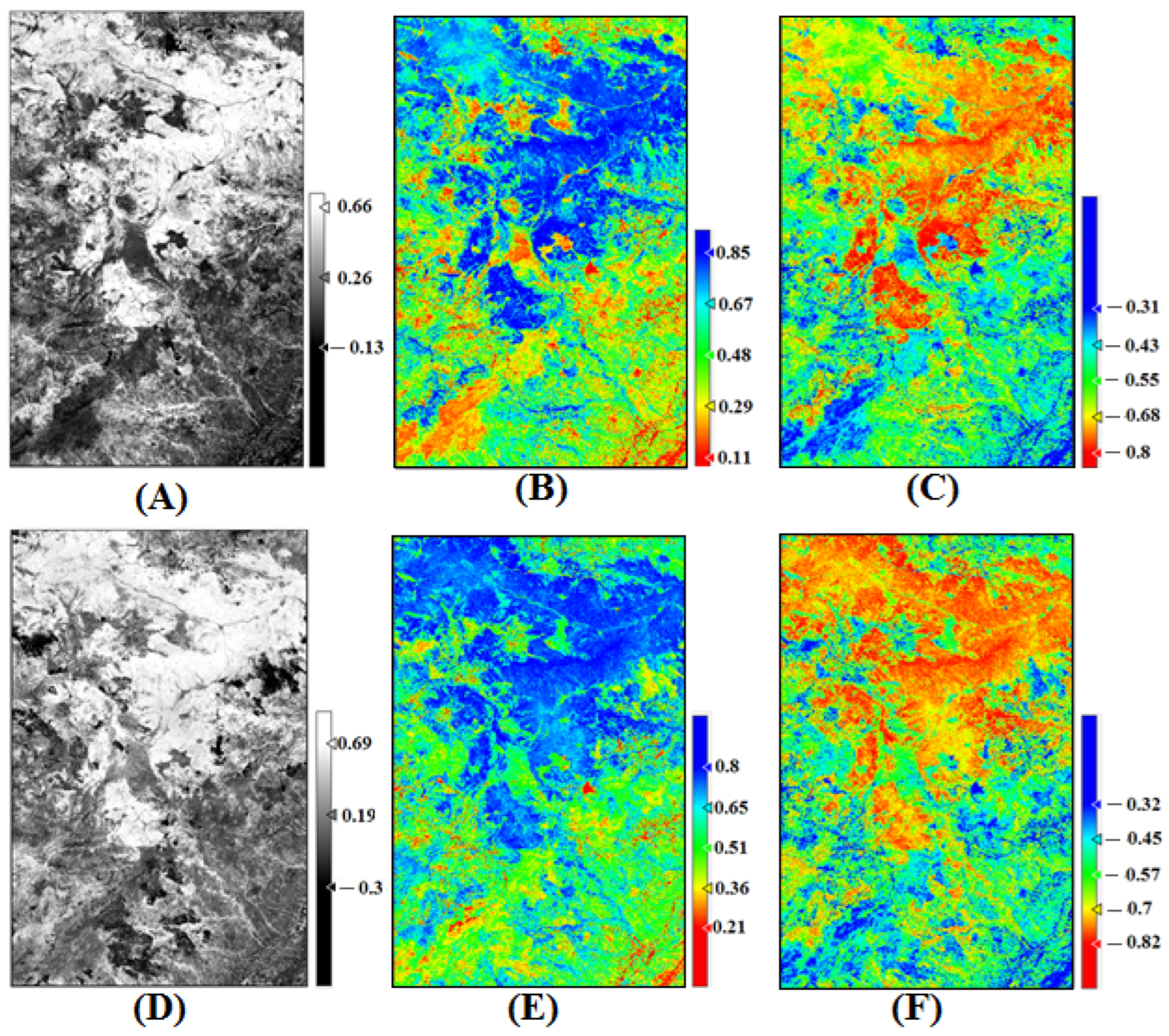
2.4.2. Preview of Fire Severity Indices Utilized

Expanding upon the analysis of scatter points between the pre-fire and post-fire images, further exploration was conducted to better discern the nuances using spectral indices. We used four indices related to fire and burnt areas (refer to Table 1) [37]. To eliminate the effects of water spectrum absorption, we also included a water area mask to remove the dark areas, which can be a source of disturbance, as reported in previous studies such as [38].
The derived dBAIS2 is the difference between pre-fire BAIS2 and post-fire BAIS2 [38].
The NDVI and NDWI calculations show spectral differences between pre-fire and post-fire images (Figure 7B,E). NDVI, derived from the NIR and red bands, highlights vegetation reflecting NIR and absorbing red light, indicating healthy growth with higher values near 1. The pre-fire image displays a larger vegetation extent (blue zones), with several areas registering high NDVI. However, notable red zones suggest unhealthy vegetation, potentially influenced by the dry climate prevalent from June in this region. This version maintains the essential information about NDVI and NDWI, spectral changes, and their interpretation in a more concise manner. The NDWI index is more sensitive to water content and shows a sharper drop in some regions of the 28 July 2020 image. This may be due to the drought conditions prevailing in the region during this period, leading to a greater loss of water content in vegetation in July compared to October (Figure 7C,F).
The NBR index allows for the identification of burn areas by utilizing the near-infrared (NIR) band, where vegetation generally reflects a significant amount of light due to its cellular structure, and the shortwave infrared (SWIR) band, where scattered vegetation reflects strongly. By comparing the pre-fire and post-fire images presented in Figure 7A,D, dark areas can be identified in the post-fire image, which may represent scattered vegetation areas after the fire. These areas do not appear in the pre-fire image.
The calculation of the dNBR (shown in Figure 8A) highlights the burn areas more clearly than the NBR index. The RBR index (shown in Figure 8B) provides a better view than the dNBR, not only for the burn areas, but also for the unburned areas. However, it can be challenging to distinguish between all the classes in the image, such as the regrowth class, which seems to merge with the unburned class.
In Figure 8C, the dBIAS2 index, which uses three vegetation red-edge bands in addition to the SWIR and red bands, highlights healthy vegetation with light shades, while burn areas are presented with dark shades. Compared to both the dNBR and RBR indices, the dBIAS2 more efficiently separates other classes, which are highlighted by the RBR index.

2.5. Fire Severity Classification

2.5.1. Fire Severity Classification Using Spectral Indices

The fire severity mapping process using the SNAP v9.0.0 application is shown in Figure 9. To perform fire severity mapping, we used a similar model to the one provided by the RUS Service in their training section “https://eo4society.esa.int/resources/copernicus-rus-training-materials/ (accessed on 3 November 2021)” but with adjusted parameters specific to our data. We also used the BIAS2 index instead of the proposed RBR index to improve the severity of fire classification.

2.5.2. Fire Severity Classification Using Machine Learning

The data processing involved the application of CNN and SVM classifiers on Sentinel-2 and Planet images. Before delving into the specifics of each method, it is crucial to understand the foundation upon which our classification process was built. The ground truth image, essential for accurate classification, was meticulously compiled using a combination of satellite data sources, including Sentinel-2 for robust spectral resolution and Planet imagery for superior spatial resolution, complemented by additional ground-based information. This comprehensive dataset, comprising spectral indices such as NDVI, NDWI, NBR, RBR, and BAIS2, alongside ground-level photographs and survey data, formed the cornerstone of our classification efforts. The ground truth image plays two roles in our study: (1) small areas of the ground truth image with uniform fire severity indices were selected to be used as “training data” in the ML methods; (2) the full ground truth image was used to evaluate how well the ML methods perform.
Both CNN and SVM used labeled training data to learn the classes of fire severity. Specifically, during the training phase, the CNN and SVM models learned the relationship between the spectral information in the selected input bands (independent variables) and the fire severity classes (dependent variables). Once trained, the models could then classify new, unseen data based on the patterns they learned.
We used the same fire severity classes for both methods. We used the SVM and CNN models in ArcGIS Pro 3.1.0. For the SVM classification, we used the Sentinel-2 and Planet post-fire images and set maximum number to 100 samples per class. For the CNN classification other parameters need to be specified. We selected U-Net, with batch size 64 and a ResNet 34 architecture. See Figure 10 for the streamflow of the approach used.

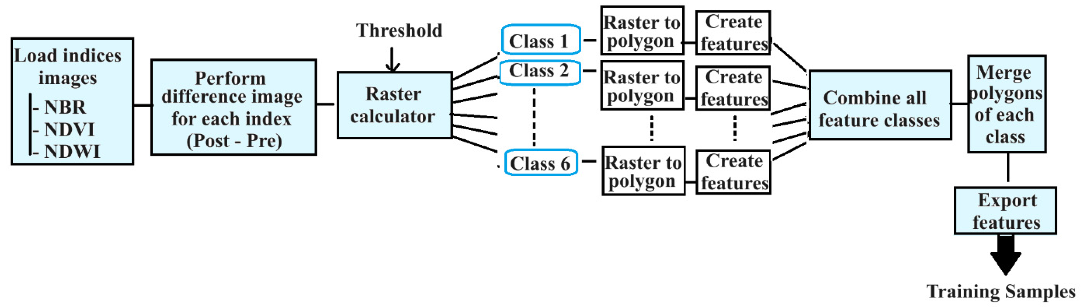
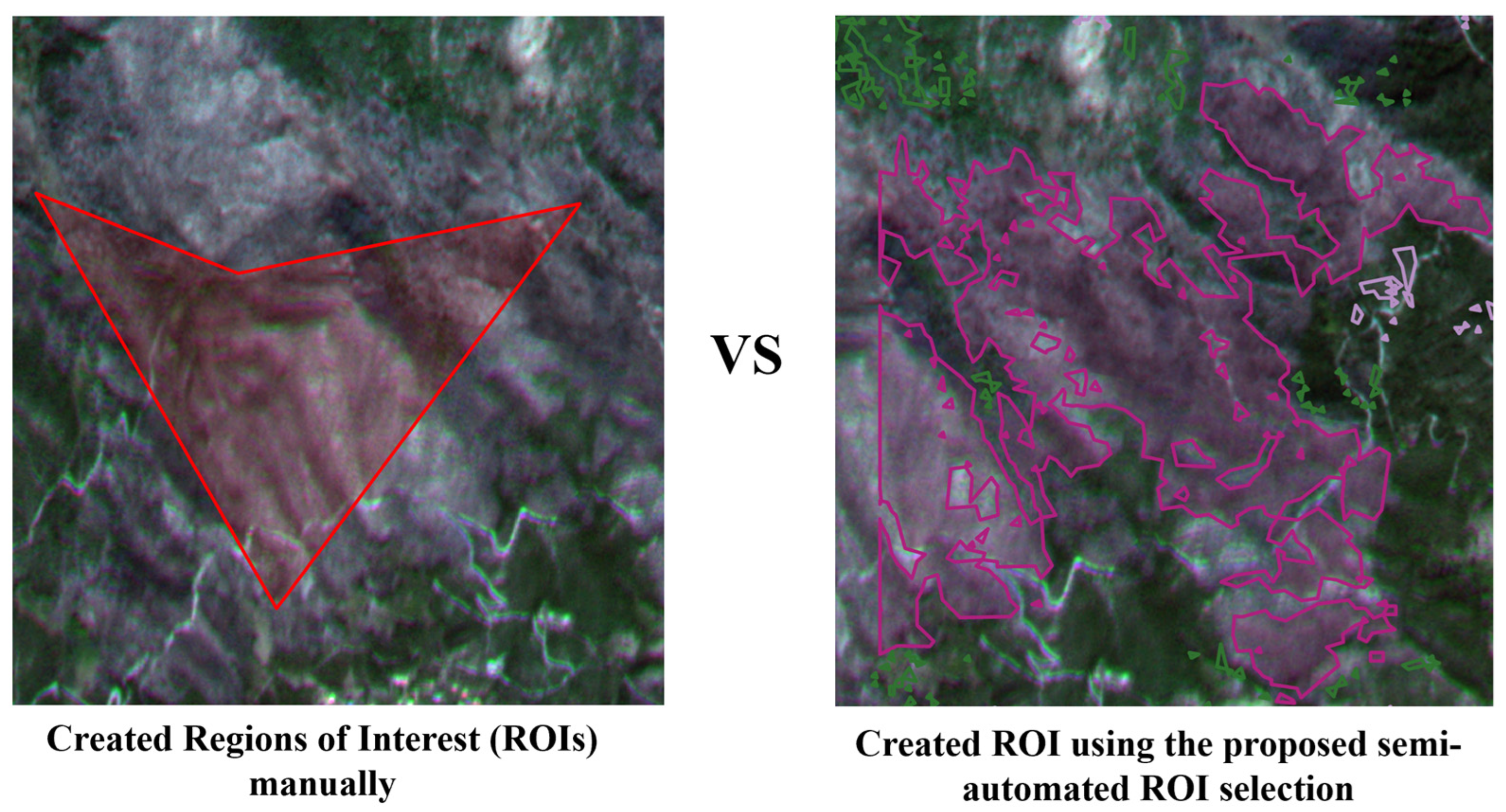
2.5.3. Training Data Labeling

The training data used in both SVM and CNN needed to reliably represent data from the study region. To achieve this, a small subset of the satellite image data needed to be labeled by the user by careful visual evaluation and identification of small regions of each of the fire severity classes. We used and compared two methods for this. The first method was entirely manual, using the ArcGIS Pro 3.1.0 default tool. The second method was a semi-automatic approach for region selection and labeling which we developed.
For the fully manual method, we first segmented the Sentinel-2 and Planet subset images using ArcGIS Pro 3.1.0 classification tools. Then, we used the training sample manager to manually create the training data. We created samples for six classes: high severity, moderate severity, low severity, unburned, high regrowth, and low regrowth. We adopted the thresholding method used by the United States Geological Survey (USGS), which defines seven fire severity categories with dNBR: high regrowth, low regrowth, unburned, low severity, moderate low severity, moderate high severity, and high severity (see Table 2).
For the second, a new semi-automatic method, we used the spectral indices’ rasters compared to the source dataset information to effectively select a generating Region of Interest (ROI) for each class. Despite the rich spatial resolution information provided by Planet imagery and the spectral index results, relying solely on this data was insufficient for creating a complete and effective map, particularly in cases involving overlapping classes and areas with canopy. Hence, we calibrated thresholds for clearly identifiable areas and applied them in ROI for training sample labeling. This approach aimed to optimize the model’s efficiency and overall performance using meticulously curated and reliable training data. By leveraging spectral index data with source dataset information for labeling, we could capture essential information that might have been overlooked during manual labeling, thereby enhancing the classifiers’ effectiveness. In Figure 11, we illustrate the principle of the semi-automated region of interest (ROI) selection in machine learning.
For the three spectral indices (BIAS2, NDWI, and NDVI), we calculated the difference between the pre- and post-indices. Next, we used raster calculation to select the rasters for each class based on the index data threshold that highlighted each of the classes. Note that this process involved manually setting thresholds for different classes by visually comparing the spectral indices results to the source dataset. In Table 3, we outline the thresholds we employed to delineate the various fire severity classes based on the results of the spectral indices dBIAS2 and dNDVI (we compare the results of the dNDVI with those of the dNDWI).
After creating different rasters for all classes, we created multiple features by fixing the feature number at 700. In cases where the raster data contain a high level of detail, converting it into a large number of features can result in overly complex and detailed polygons. Fixing the number at 700 features is a way to simplify the output for easier visualization and analysis and to manage the size of the output dataset. We merged the rasters of the same classes and combined all classes into one image. It is important to note that we only utilized 20% of the data for training, ensuring a manageable dataset. The process is shown in Figure 12.
To prepare the data for the machine learning training, we performed a raster-to-vector conversion, obtaining the shapefile necessary for the training process. A comparison between the resulting ROI generated using the proposed semi-automated ROI selection and a manually selected ROI based on ground truth examination is presented in Figure 13.
Additionally, when exporting the data for the CNN training, we carefully chose the “Classified tiles”, which are masks explicitly crafted to emphasize pertinent features and improve the CNN’s learning process. For the pixel classification task, we selected the U-Net model. It consists of a contracting path to capture context and a symmetric expanding path to enable precise localization. As for the ResNet-50 architecture, we chose it for its deep network architecture with 50 layers, which allows it to learn more complex features from the data, potentially leading to improved classification performance. Throughout the experimentation, we employed a GPU with 8 GB of memory for processing, which significantly accelerated model training and inference compared to using a CPU.
As is known in CNNs, achieving optimal performance demands a substantial volume of labeled samples due to their ability to capture intricate patterns, requiring extensive exposure for optimal functioning. Despite their potency and vast parameter space, effective methods for sample selection are essential. Meticulous training sample selection is crucial for CNNs. While our proposed semi-automated method for selecting Regions of Interest (ROIs) has shown promise in outperforming manual selection methods, a critical aspect that remains unclear is the optimal number of samples required for effective performance. To address this gap, our experiment focused on determining the ideal sample size needed to enhance the efficiency of this method. Specifically, we aimed to investigate various percentages of spectral raster data from each class (e.g., 10%, 20%, and 50%) to identify the most effective input configuration for the training process.
In the semi-automated ROI selection with SVM context, strategic spectral rasters for ROI selection becomes crucial. In this instance, fractions such as 0.1%, 10%, 20% and 50% of the spectral rasters were carefully chosen. Remarkably, as the selection process progressed to encompass 20% of the available data, notable convergence occurred in the results. This convergence led to an improvement in the accuracy for both the Sentinel-2 and Planet images when employing the semi-automated indices-based method with SVM (Figure 14A,B). However, the CNN method, when subjected to similar spectral raster selection, revealed a contrasting outcome. Here, the selected approach did not yield optimal results (see Figure 14C,D), with one of the classes consistently missing from the final output.
A consequential observation emerged in the context of the “regrowth” and “unburned” classes for the CNN method. These two classes exhibited an abundance of samples, and this abundance inadvertently overshadowed the remaining classes. Recognizing this, we adjusted our approach to balance the number of spectral rasters allocated to each class.
By recalibrating the distribution of spectral rasters among classes, a more equitable representation was achieved, thereby mitigating the issue of certain classes being overshadowed by the dominance of others. We ultimately adopted this selection approach for the semi-automated ROI indices-based methods.

3. Results

We evaluated the outcomes from both methods by comparing them with ground truth data. This involved cross-referencing the classified maps with observed ground truth information to assess their accuracy in mapping fire severity.

3.1. Evaluation Parameters

In this section, we discuss the evaluation parameters utilized to assess the performance of our fire severity mapping methods. Firstly, we calculated the separability index (SI) for the images generated from the Relative Burn Ratio (RBR) and dBIAS parameters. The SI serves as a metric to quantify the ability of these spectral indices to differentiate between different fire severity classes [38]. A higher SI value indicates better separability, implying that the spectral indices are effective in distinguishing between varying degrees of fire severity.
Separability Index (SI): The separability index is a measure of the degree of separability between two classes based on their mean values and standard deviations [38], using the formula:
S I = μ b μ u ( σ b + σ u )
where:
-
μ b and μ u are the mean values of the considered indices for the burnt and unburnt areas, respectively;
-
σb and σ u are the standard deviations for the burnt and unburnt areas.
While SI is a valuable tool for assessing the discriminatory power of spectral indices, it is not applicable to ML-generated images. This is because ML methods, such as SVM and CNN, operate differently from spectral indices. ML classifiers learn patterns and relationships directly from the data during training, making the concept of separability less relevant. Therefore, SI calculation is not performed for ML-generated images, and precision-recall analysis serves as a more appropriate evaluation metric for these models. Building upon this, we undertook an assessment of the accuracy for SA-ROI-based classification and machine learning classification (SVM and CNN) using the ArcGIS Pro 3.1.0 software. This entailed a validation process where all accuracy assessment points were compared with the ground truth image. The calculated parameters included:
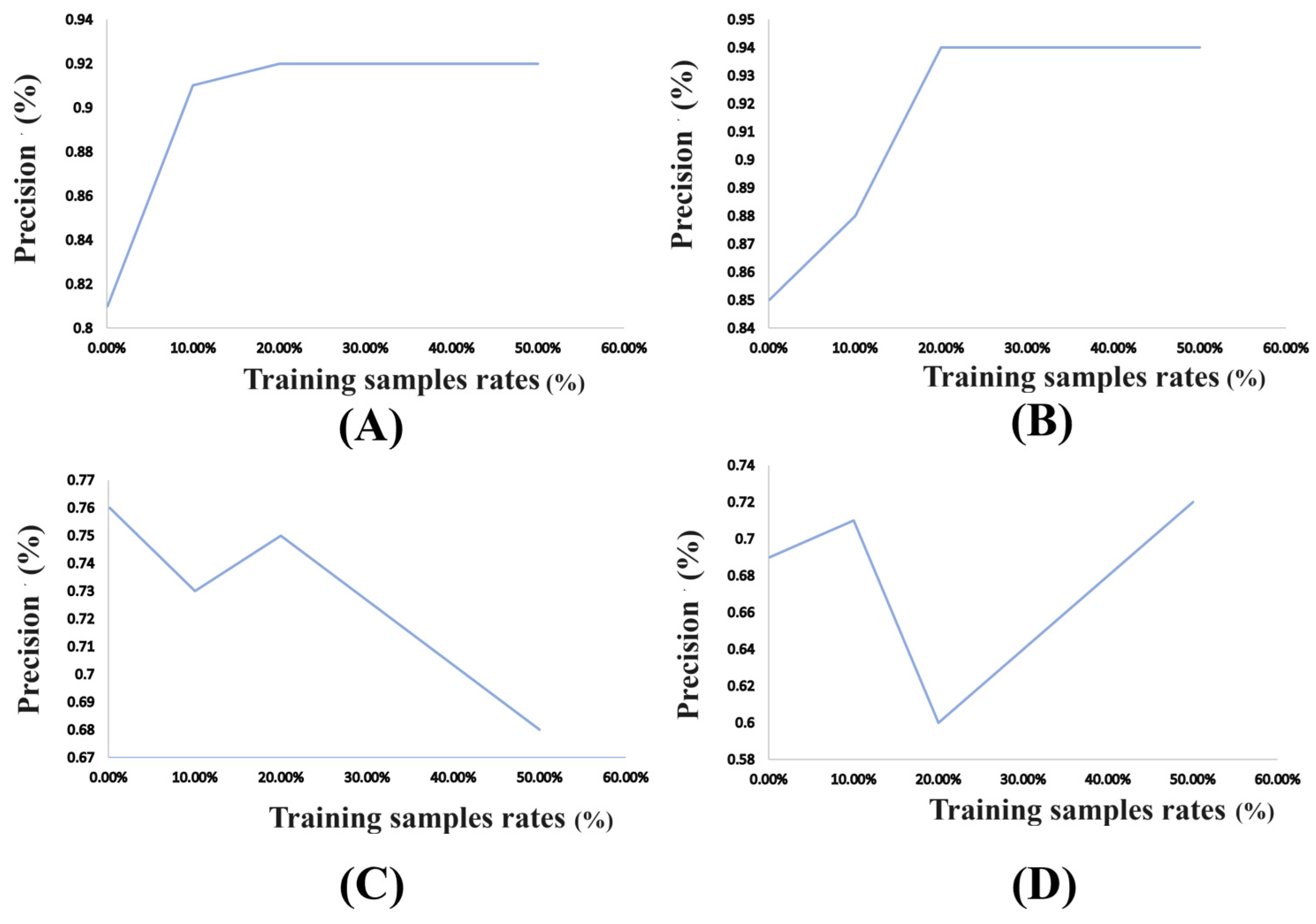
Precision: Precision is a metric used to evaluate the performance of a binary classification model, specifically focusing on the accuracy of positive predictions. It measures the proportion of true positive predictions (correctly predicted positive instances) out of all positive predictions made by the model. It is given by Equation (2).
P r e c i s i o n = T r u e   P o s i t i v e s ( T r u e   P o s i t i v e s + F a l s e   P o s i t i v e s )
where:
-
True Positives (TP) are the instances that are correctly predicted as positive;
-
False Positives (FP) are the instances that are wrongly predicted as positive when they are actually negative.
Recall: Recall measures the proportion of true positive predictions (correctly predicted positive instances) out of all actual positive instances in the dataset. It is given by Equation (3).
R e c a l l = T r u e   P o s i t i v e s ( T r u e   P o s i t i v e s + F a l s e   n e g a t i v e s )
The Overall Accuracy: The Overall Accuracy is the average precision. It is given by Equation (4).
O v e r a l l   A c c u r a c y = ( T r u e   P o s i t i v e s + T r u e   N e g a t i v e s ) ( T r u e   P o s i t i v e s + T r u e   N e g a t i v e s + F a l s e   P o s i t i v e s + F a l s e   N e g a t i v e s )
where:
-
True Negatives (TN) are the instances that are correctly predicted as negative;
-
False Negatives (FN) are the instances that are wrongly predicted as negative when they are actually positive.
The F1 score: The F1 score is a metric commonly used to evaluate the performance of binary classification models, particularly when there is an imbalance in the distribution of classes. It combines precision and recall into a single value, providing a balanced measure of the model’s accuracy. The equation for calculating the F1 score is as follows:
F 1   s c o r e = 2 × ( P r e c i s i o n × R e c a l l ) ( P r e c i s i o n + R e c a l l )
Kappa coefficient: The kappa coefficient measures the agreement between an observed set of class labels and the predicted set of class labels assigned by a classifier. It considers both the accuracy of the classifier and the agreement that could occur by chance. The kappa coefficient is calculated using the following formula:
Kappa = ( P 0 P e ) / ( 1 P e )
where:
-
P 0 is the observed agreement, which is the proportion of instances where the observed and predicted labels match;
-
P e is the expected agreement, which represents the agreement expected by chance.

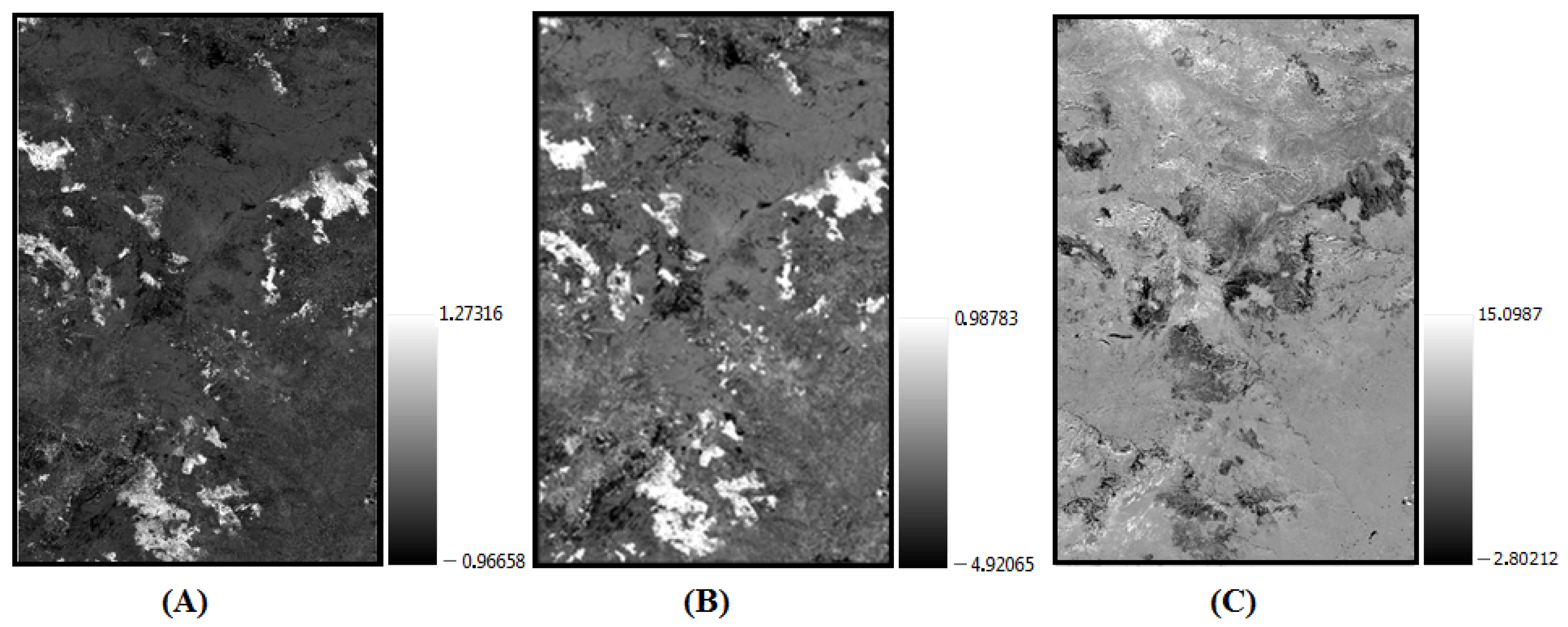
3.2. Index-Based Results

The Sentinel-2 pre–post difference image and its segmented image are given in Figure 4. The generated fire severity results using RBR and dBIAS2 were classified into six classes.
The maximum value given by our selected study area is 0.98. Since the values for the “Moderate high severity” and “High severity” classes were very close, with only a small difference between them, we decided to merge these two classes into a single class, which we named “High severity”.
The visual inspection of the two sets of image results showed that the fire severity classes (low severity, moderate severity, and high severity) were well classified. In particular, the dBIAS2 results (Figure 15C) highlight these classes better than the RBR results (Figure 15B), which exhibit some overlap between the low-severity and moderate-severity classes. Moreover, the RBR results show that the vegetation information appears almost as one class, i.e., the unburned class.
Both the RBR and dBIAS2 indices were assessed for SI, as detailed in Table 4, revealing dBIAS_SI = 1.084 and RBR_SI = 0.405. An SI value greater than 1 signifies good separation of burned area classes, while a value less than 1 indicates poor separation. These SI results reinforce the findings obtained from visual inspection.
Despite these results in favor of the dBIAS2 index’s effectiveness in certain areas, it misclassified a significant portion of the image information when compared to the reference image (pre–post difference image presented in Figure 15A).

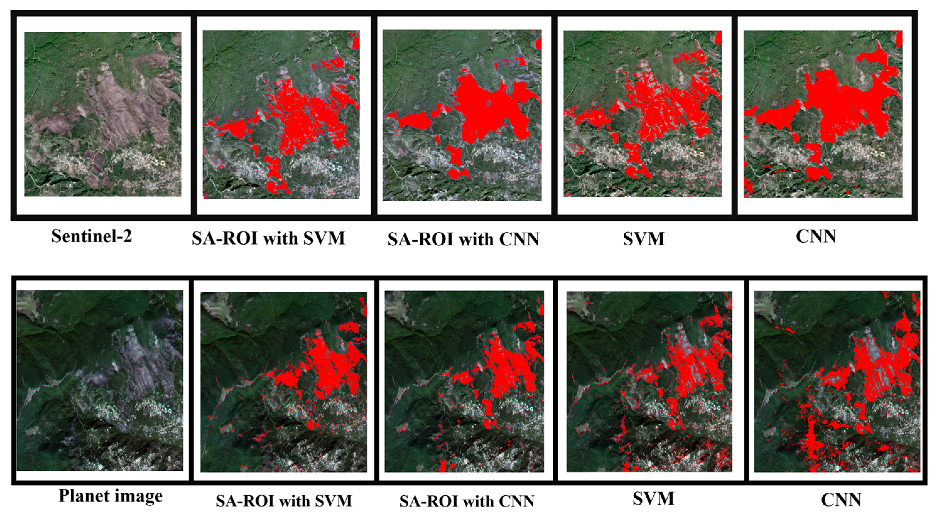
3.3. Machine Learning-Based Method Results

The outcomes of the machine learning methods distinctly exhibit improved class separability compared to the RBR and dBIAS indices. The resultant images more closely align with the ground truth. The fire severity classification results for Sentinel-2 images using SVM and CNN methods are shown in Figure 16B,C, while those for Planet images using SVM and CNN are displayed in Figure 16D,E.
Comparing the false-color image in Figure 16A with the results of the SVM and CNN classified images in Figure 16B–E, most classes in the image are prominently highlighted, exhibiting similar shapes in both SVM and CNN classified images. However, notable differences arise in the CNN image, particularly in regions 2 and 4, where misclassification as “high regrowth” occurs.
Additionally, the CNN classified image minimally represents the “low severity” class compared to the SVM classified image. Obtaining precise details in the image, especially for small areas, poses challenges due to Sentinel-2’s spatial resolution. To ensure accuracy, we cross-verified using higher-resolution references such as the Planet image, Google Earth map, on-site survey data, and region photos. These sources offered higher spatial resolution and more precise information.
Upon inspection, the CNN model classified the north part of the area (region 1) as “high regrowth”, which contradicts the presence of settlements in this area, indicating low regrowth. Notably, both the SVM and CNN models misclassified this area using the Planet image (Figure 16B,E). Conversely, areas classified as “low severity” by SVM with Sentinel-2 images included developed areas, bare soils, or areas with poor regrowth. Visual assessment suggests SVM with Sentinel-2 images presents better results.
However, upon comparison with ground truth data, an intriguing observation emerged. Specifically, both SVM and CNN classified the surroundings of unburned areas, such as in region 3, as having moderate severity. Yet, high-resolution analysis using the Planet image revealed these areas primarily consist of trees and plants, indicating they should be classified as unburned areas. We suspect this misclassification may stem from the canopy effect caused by the area’s topography and reflective properties of the satellite’s sensors, contributing to misinterpretation of these regions.
The results showed that the Sentinel-2 image outperformed the Planet image in terms of accuracy, despite the higher spatial resolution of the latter. This is because this kind of application requires rich spectral band information, especially the SWIR band. It is crucial to use both spatial and spectral features to produce accurate fire severity classifications and burned area maps [42].
It is important to note that accurately differentiating the six different classes in the image based only on the ground truth image is difficult for this kind of application. Manual selection of Regions of Interest (ROIs) solely based on visual examination of satellite images, even with high-resolution ones, particularly for regions exhibiting mixed classes, presents difficulties in terms of achieving optimal results with machine learning (ML) methods.
The spectral indices (RBR, NBR, NDVI, NDWI, and dBIAS) provided crucial pre-knowledge of the different classes, especially for the severe classes. Using the indices is a good guide for selecting ROIs for training data. However, manually selected ROI (MS-ROI) is challenging, which motivated our development of the semi-automatic (SA-ROI) method.
The SA-ROI method with SVM used on the Planet image demonstrated promising results closely resembling our ground truth data, notably in the four selected zoom regions (refer to Figure 17D). Comparable outcomes were observed with the same SA-ROI method using SVM applied to the Sentinel-2 image. However, with this image, regions 1 and 4 show comparatively poorer results in Figure 17B. Contrastingly, employing the SA-ROI method with CNN yielded less favorable results for both Sentinel-2 and Planet images. Regions 1, 2, and 4 exhibited misclassifications (refer to Figure 17C,E).
It is important to highlight that results from the CNN and SVM methods using both Sentinel-2 and Planet images exhibited sensitivity to canopy effects, resulting in incorrect classifications. However, the SA-ROI methods using SVM and CNN with both the Sentinel-2 and the Planet images showed reduced sensitivity to these effects, particularly excelling in classifying regions with dense canopy cover, such as region 3. Notably, when employing the SA-ROI method with SVM on the Planet image dataset, superior classification efficiency was observed.

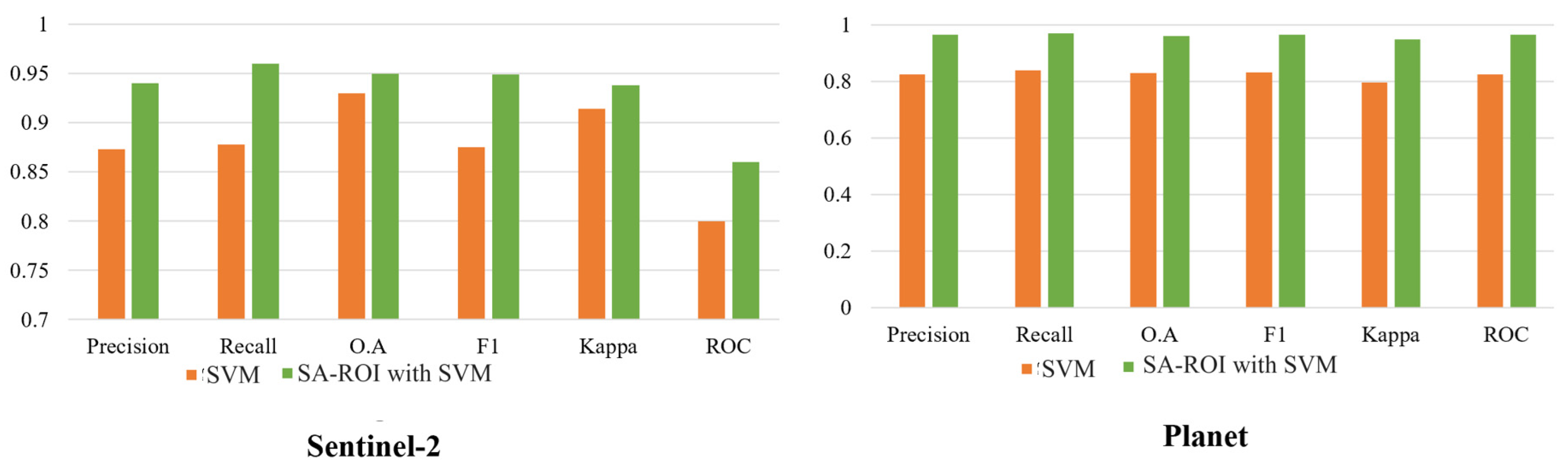
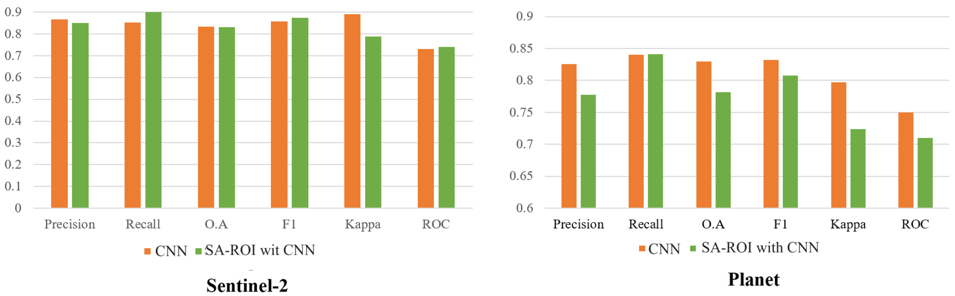
3.4. Quantitative Accuracy Assessment

3.4.1. A Comparative Accuracy Assessment
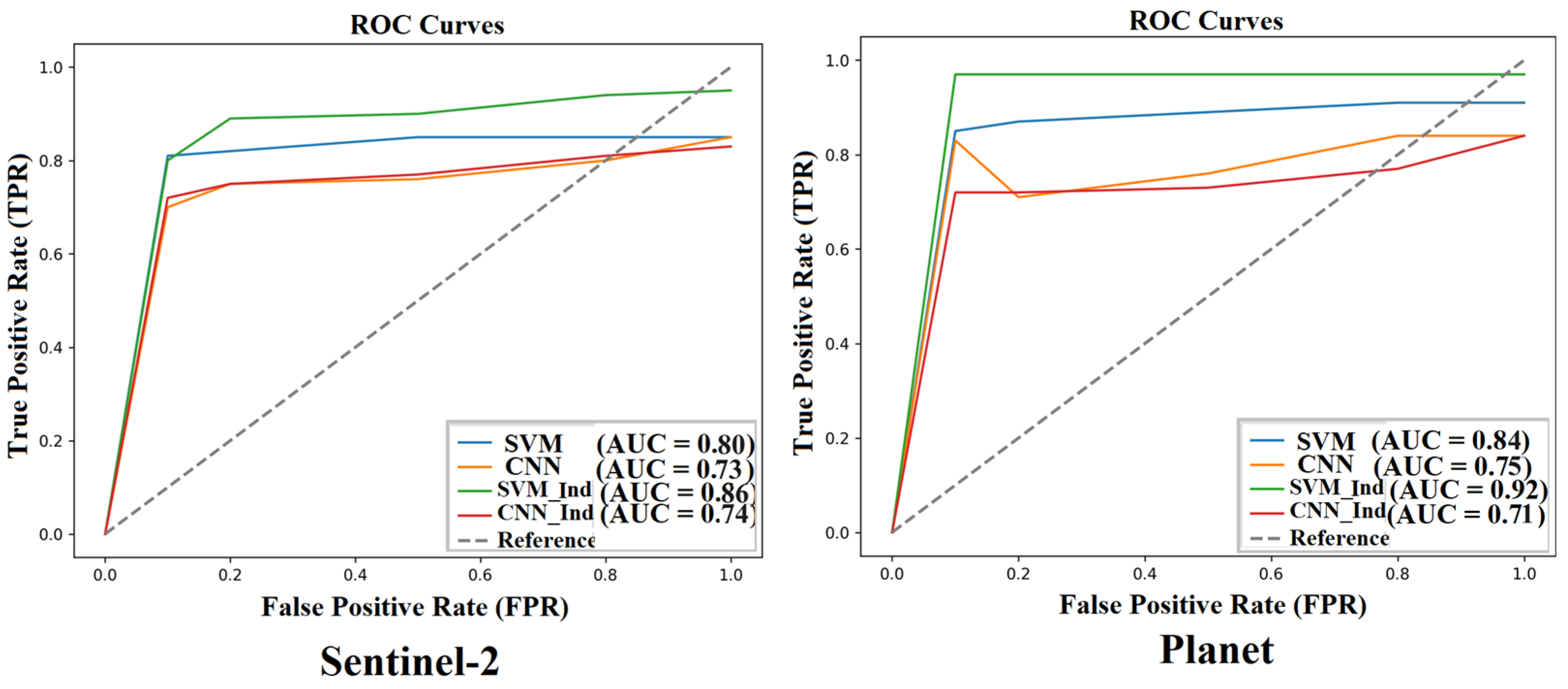
The accuracy assessment for the RBR and dBIAS indices is presented in Table 5. The dBIAS index exhibited better results, achieving a precision of 0.771, a recall of 0.620, an F1 score of 0.687, a Kappa of 0.788, and an overall accuracy (OA) of 0.831. In comparison, the RBR index demonstrated a precision of 0.541, a recall of 0.542, an F1 score of 0.541, a Kappa of 0.337, and an overall accuracy (OA) of 0.475. The SVM method applied to the Sentinel-2 image achieved higher assessment accuracy, with a precision of 0.873, a recall of 0.878, a Kappa of 0.914, an F1 score of 0.875, and an overall accuracy (OA) of 0.930 (refer to Table 5). However, competitive results were also obtained by the CNN method.
A noticeable enhancement in accuracy is evident from the outcomes tabulated in Table 5. The most favorable accuracy, presented in bold format in Table 5, was achieved by the SA-ROI method coupled with SVM, particularly when applied to the Planet image. This configuration demonstrated a recall of 0.970, precision of 0.966, overall accuracy of 0.960, an F1 score of 0.967, and a Kappa value of 0.950.
While the pinnacle accuracy favored the Planet image, it is essential to underscore that the training samples primarily stemmed from the Sentinel-2 image due to the inclusion of the SWIR band in this dataset.

3.4.2. ROC Curves

The results demonstrated a high level of accuracy, especially for the SA-ROI method with SVM. This approach showed an improvement in accuracy compared to SVM with both Sentinel-2 and Planet images, as presented in Figure 18. According to Swets (1988) [43], an AUC (Area Under ROC Curves) value exceeding 0.7 is considered a critical threshold indicative of practical utility in real-world applications. All the classifiers yielded interesting results with high accuracies. Notably, the lowest AUC values were observed, with AUC = 0.73 for Sentinel-2 and AUC = 0.71 for Planet images in the case of CNN and the SA-ROI method with CNN, respectively (refer to Figure 18 for Receiver Operating Characteristic (ROC) curves). It is worth noting that the results with the CNN method are somewhat surprising and may not meet expectations. Despite the effectiveness of the training sample selection demonstrated with SVM, the CNN method did not show significant improvement. This could be attributed to various factors, such as tuning parameters, network architecture, or limitations of the ArcGIS Tool.
It is well-known that CNN methods often yield superior results, as they are designed to recognize relationships in data through learning from labeled training samples. Given that spectral indices alone proved insufficient with a randomly selected indices-based training model, a more efficient selection based on the study of relationships between samples might enhance CNN results. This presents a promising avenue for future research.
From the results obtained, the SA-ROI method with SVM stands out, achieving the highest precision with an AUC of 0.86 for Sentinel-2 and an impressive AUC of 0.92 for Planet images (refer to Figure 18).

3.4.3. Burned Area Extent

The area and percentage that fell in each fire severity class for all the methods used are presented in Figure 19 and Figure 20. It can be observed that, except for the spectral index RBR (Figure 19A and Figure 20A), the total rates of the vegetation and severe classes led to similar values across all methods. Specifically, the total rates of the three severe classes range from a minimum of 19% in the case of Sentinel-2 image with SA-ROI method with CNN to a maximum of 40% in the case of Planet images with SVM.
In terms of vegetation rates, an interesting observation emerges when considering the SA-ROI and machine learning methods. Although the overall rates exhibit close proximity, divergence becomes evident when examining the rates for the three distinct vegetation classes. Notably, the class labeled as “low regrowth” attained its highest value when employing the dBIAS approach (as depicted in Figure 19B and Figure 20B), while the “high regrowth” class achieved its peak value in the context of the Sentinel-2 CNN method (as seen in Figure 19D and Figure 20D).
Conversely, a consistency in values arose with Sentinel-2 and Planet images, where both SVM and CNN produce similar rates for all three vegetation classes. These values are depicted in Figure 19C,D,G,H and Figure 20C,D,G,H.
Turning our attention to the SA-ROI methodologies, intriguing insights emerge. Notably, the unburned class exhibited higher rates when compared to the machine learning methods, while the moderate severity class registered lower rates (See Figure 19E,F,I,J and Figure 20E,F,I,J). This discrepancy can be attributed to the efficacy of semi-automatic approaches in identifying areas that were initially misclassified as having moderate severity. This misclassification is often tied to the presence of dense canopy cover and the influence of satellite detector reflections. Consequently, the semi-automatic methods excelled in rectifying these misclassifications, thereby yielding higher accuracy in detecting unburned regions and reduced accuracy in moderate severity regions.

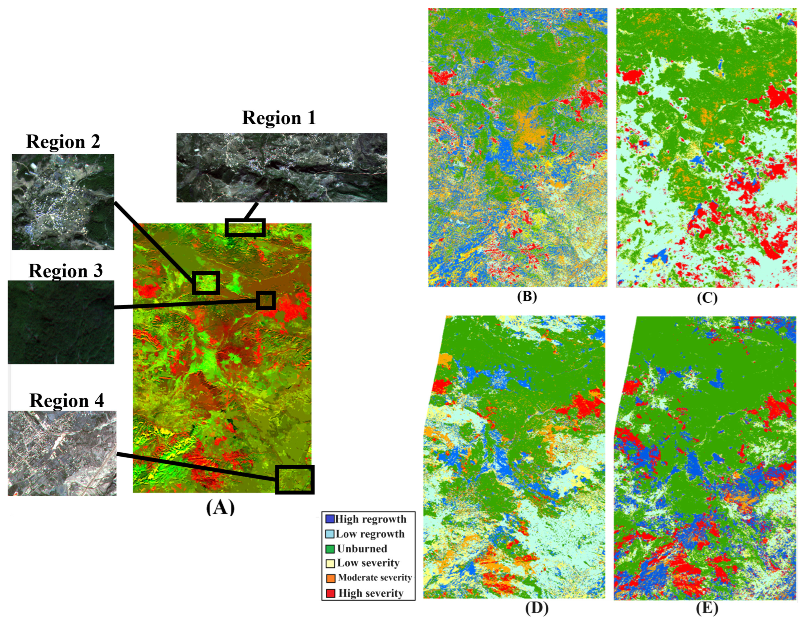
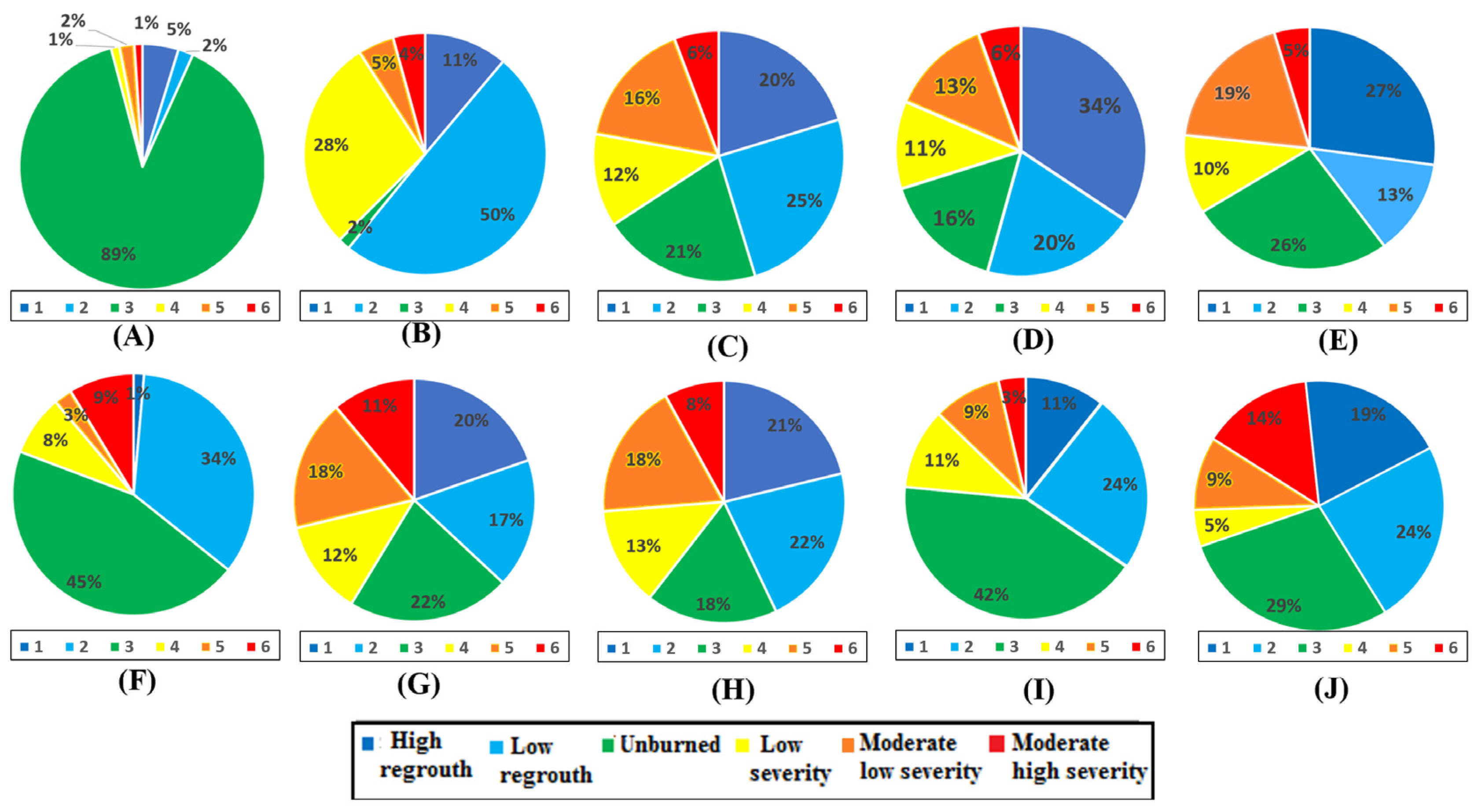
3.5. High Severity Map

After generating the fire severity maps using all proposed methods, we compared the high-severity map for both Sentinel-2 and Planet images. Figure 21 depicts the high-severity map for all the proposed methods.
Following the generation of fire severity maps using all the proposed methods (Figure 21), we conducted a visual evaluation of the resulting high-severity map across several burned areas, as delineated in Figure 22. The burn areas were zoomed in on in the selected study area for Sentinel-2 and planet images. The high-severity areas were correctly classified by all the proposed methods, as shown in Figure 21. The Sentinel-2 CNN, Sentinel-2 semi-automatic with SVM, and Planet semi-automatic with SVM appeared to produce the most favorable results. However, while other methods successfully identified most high-severity areas, there was an overestimation of this class for the SVM and SA-ROI-CNN and an underestimation for the case of RBR.

3.6. Relation to Influencing Parameters

Due to the diverse topography of the study area, it is challenging to categorize the resulting classes into distinct ranges. However, it is noticeable that the high-severity class was predominantly located in the elevation range of 500 m to 1500 m, with a slope range of 25° to 40° and a mean wind speed of 9 m/s. In terms of aspect, most of the high-severity fire area was concentrated in the cities of Adekar and Idjeur, covering an area of nearly 979 hectares with an aspect range of 157.5 to 202.5 degrees. Notably, this area represents the largest proportion of the high-severity class. The remaining parts of the high-severity class were distributed across various locations, with a highly variable aspect range. The yearly average temperature and precipitation for the high-severity area are 19 °C and 17%, respectively.

4. Discussion

The effectiveness of the supervised machine learning algorithms heavily relied on the quality of the training data. Our proposed methodology sought to optimize the selection of training data by leveraging spectral indices to highlight regions of interest (ROIs) in a precise manner across diverse land classes.
Comparative analysis between classical spectral indices such as RBR and dBIAS2 for fire severity and machine-learning-based classification unveiled the limitations of relying solely on spectral indices, which often focus on isolated indices. In our study, we calculated NDVI and NDWI to emphasize the unburned classes, while dBIAS highlighted the burned classes. Each spectral index served to emphasize a specific class in the context of fire severity assessment. Contrarily, machine learning methods considered the holistic context of data, demonstrating superior capacity in recognizing broader patterns beyond spectral characteristics. Yet, manual labeling during training poses challenges, particularly in contexts like fire severity, where complex details may be missed in real images.
Integrating spectral index results with ground truth data from satellite imagery (Planet and Sentinel-2), pre–post difference, and segmented images alone is inadequate for comprehensive mapping, especially in areas with overlapping classes and canopy cover. To address this, we calibrated thresholds for distinct areas and applied them to ROI for machine learning training. This optimization strategy enhanced model efficiency and performance by incorporating reliable training data, combining spectral indices with source dataset information for labeling. This approach ensures a more effective classification by capturing crucial details that manual labeling might overlook. Our proposed semi-supervised approach utilizing spectral indices for semi-automated labeling displayed promising results, especially evident in the SVM classifier. Notably, our method significantly enhanced accuracies and ROC values for both Sentinel-2 and Planet datasets, showcasing its potential to improve machine learning outcomes (Figure 23).
Although the SA-ROI method coupled with the SVM classifier showcased a noticeable improvement and offered enhanced ROI quality for training data selection, the outcomes observed with the CNN classifier were unexpected. Surprisingly, while a marginal increase in accuracy was evident for the Sentinel-2 image using the spectral indices-based method with the CNN classifier, a decline in accuracy was noted for the Planet image when compared to the CNN results alone (Figure 24). Several factors could contribute to this divergence, including the tuning parameters of the CNN, its architecture, data augmentation, potential limitations within the CNN parameters provided by the ArcGIS Pro toolbox, or other variables. Nonetheless, this disparity represents a significant limitation of this study.
An additional concern regarding the proposed method is the arbitrary selection of spectral index rasters for ROI generation in the training data selection process. Implementing advanced techniques, such as similarity analyses of class spectra, to guide the optimal selection of spectral index thresholding could potentially enhance the outcomes of the method.
These findings, particularly the unexpected outcomes observed with the CNN classifier and the potential limitations identified in the selection of spectral index rasters for ROI generation, may pose new challenges for future research endeavors.
In contrast to the methodology in reference [35], which employed an automatic processing chain for burned area segmentation using mono-temporal Sentinel-2 imagery and focused on a convolutional neural network based on a U-Net architecture, our approach emphasizes the use of generated spectral index rasters to efficiently highlight the ROIs for all classes, extending beyond burned and unburned categories. This diversification enhanced the inputs for our machine learning model during training. Notably, our method classified the burned and unburned areas into three severity degrees, offering a more nuanced and versatile map suitable for applications like land use and land cover mapping. While the segmentation model in [35] achieved an impressive overall accuracy of 0.98 and a kappa coefficient of 0.94, our method yielded competitive accuracy results. We addressed challenges like water bodies and shadow effects through preprocessing steps using band maths in SNAP v9.0.0, eliminating potential hindrances encountered by [35]. Despite [35] covering smaller areas from different regions globally, our work’s generalization to various regions remains a perspective for future exploration, providing a comprehensive evaluation of its applicability.
The integration of spectral indices in ROI selection for machine learning training in remote sensing data analysis represents a theoretical advancement, refining classification methodologies to address challenges in overlapping classes and canopy-covered areas. This approach, combining spectral indices with source dataset information for labeling, offers a practical solution for enhancing the accuracy of mapping in complex landscapes. The semi-automatic spectral indices-based ML methods ensure reliable classification results, making the methodology valuable for applications such as environmental monitoring, land management and disaster response. By leveraging machine learning methods and meticulously curated training data, the proposed approach provides an efficient and effective tool for optimizing mapping efforts in diverse geographical contexts.
One of the important applications, as demonstrated in this work, is fire severity classification, with the added utility of preventing wildfires. Factors such as weather conditions, human activities, and landscape characteristics play significant roles in the spread and severity of wildfires in our study area. However, it is likely that the highly severe areas (moderate and high severe classes) identified in 2020 could have become fuel sources for fires in the surrounding regions in the subsequent years (see Figure 25). This phenomenon is commonly observed in fire ecology, where areas affected by previous fires can act as fuel for future fires, particularly if vegetation regeneration has not had sufficient time or if fire management practices are inadequate [44]. To verify this, we downloaded the Planet images for the three subsequent years (after 2020), and we checked for fire activity in this region using the FIRMS website “https://firms.modaps.eosdis.nasa.gov/map (accessed on 15 March 2024)” to identify detected fires in these years. Indeed, fire activity in the following years was observed to be close to or around the identified high-severity classes. Some of these fires persisted for more than 24 h after detection (highly dangerous). Our proposed method may not only facilitate efficient classification of fire severity, but also contribute to effective fire management by removing dead trees and vegetation that fuel large fires. Planting new seedlings is another critical aspect of this effort.

5. Conclusions

Our study focused on fire severity classification within the Akfadou forest in Northern Algeria. We conducted a comparative analysis of two spectral parameters, the Relativized Burn Ratio (RBR) and the Difference from Burned Reference Index (dBIAS), in conjunction with machine learning methods such as CNN and SVM using ArcGIS Pro 3.1.0. Our results demonstrated strong performance, particularly for high-severity classes, with both SVM and CNN methods achieving accuracy scores exceeding 0.84.
Our work introduces an innovative approach to training sample labeling, addressing challenges in accuracy and efficiency. By leveraging spectral indices data and an active learning process, we optimized the selection of rasters for six distinct classes. Manual labeling can be labor-intensive and prone to inaccuracies, especially in capturing fine details. In contrast, our approach systematically curated training data, ensuring its accuracy and capturing essential information often overlooked in manual labeling. This approach notably enhanced the accuracy of the semi-automatic indices-based method with SVM and improved classification efficiency, particularly in mitigating the canopy effect.
However, while the semi-automatic indices-based method with CNN showcased effectiveness in addressing the canopy effect, it did not yield significant accuracy improvements, with certain areas still experiencing misclassifications. There is potential for further improvement by fine-tuning the model parameters and exploring newer architectures and different models may also enhance the method’s efficiency.
Another issue with this proposed method is the random selection of spectral index rasters for ROI creation. Optimal selection based on similarity analyses of class spectra, using advanced techniques like spectral graph-based methods [45,46] or spectral metrics [47,48] might yield superior results. Additionally, determining the best threshold for spectral index selection can prevent overlaps and enhance accuracy. Exploring additional spectral indices can offer supplementary data that may further improve classification accuracy.
Our study provides a detailed analysis of the study area. Specifically, our results indicate that at least 1627 hectares of the Akfadou forest are classified as severe burn areas. These areas may also act as fuel sources for the surrounding regions in the subsequent years. This forest is known for its diverse flora and rare species, and urgent measures are needed to restore the damaged areas. This may involve vegetation establishment through re-seeding or replanting processes with native species.
Our study has made substantial progress in fire severity classification, automation of training data labeling, and the exploration of innovative techniques. Continued research and refinement in these areas present exciting opportunities for further enhancing the accuracy and efficiency of fire severity mapping, with potential applications extending to broader environmental and land management initiatives. It is important to note that the study area represents a single site within a single year, chosen to aid in result verification and method validation. As we move forward, it is essential to consider expanding our research to encompass larger areas across different time series. This broader scope will allow us to generalize and refine our methodology, ultimately contributing to a more comprehensive understanding of fire severity mapping and its practical applications.

Author Contributions

N.Z. (Principal Author) led the research project, conducted data analysis, and authored the manuscript, and collaborated with all co-authors and incorporated their contributions into the study. H.R. actively participated in discussions, contributing valuable insights and ideas throughout the research process, including aiding in data treatment, paper writing, and paper structuring. M.I.C. made important contributions by suggesting additional experiments, resulting in improved methodology and enhanced results. T.K. provided guidance on data acquisition and materials, reviewed satellite data, and offered valuable input. N.R. conducted an analysis of research results, identifying areas for improvement in both methodology and interpretation. M.L. assisted in data verification and statistical analysis and offered general observations that enriched the research. All authors have read and agreed to the published version of the manuscript.

Funding

This research received no external funding.

Data Availability Statement

All data and steps of the developed algorithm were processed in ArcGIS Pro and SNAP. Unfortunately, we are unable to share these data at this time. However, we are considering developing the proposed method into a toolbox, which we hope to accomplish soon.

Conflicts of Interest

The authors declare no conflicts of interest.

References

  1. Kideghesho, J.; Rija, A.; Mwamende, K.; Selemani, I. Emerging issues and challenges in conservation of biodiversity in the rangelands of Tanzania. Nat. Conserv. 2013, 6, 1–29. [Google Scholar] [CrossRef]
  2. Gibson, R.; Danaher, T.; Hehir, W.; Collins, L. A remote sensing approach to mapping fire severity in south-eastern Australia using sentinel 2 and random forest. Remote Sens. Environ. 2020, 240, 111702. [Google Scholar] [CrossRef]
  3. Keeley, J.E. Fire intensity, fire severity and burn severity: A brief review and suggested usage. Int. J. Wildland Fire 2009, 18, 116–126. [Google Scholar] [CrossRef]
  4. Díaz-Delgado, R.; Lloret, F.; Pons, X. Influence of fire severity on plant regeneration by means of remote sensing imagery. Int. J. Remote Sens. 2003, 24, 1751–1763. [Google Scholar] [CrossRef]
  5. Wen, D.; Huang, X.; Bovolo, F.; Li, J.; Ke, X.; Zhang, A.; Benediktsson, J.A. Change detection from very-high-spatial-resolution optical remote sensing images: Methods, applications, and future directions. IEEE Geosci. Remote Sens. Mag. 2021, 9, 68–101. [Google Scholar] [CrossRef]
  6. Stomberg, T.; Weber, I.; Schmitt, M.; Roscher, R. Jungle-net: Using explainable machine learning to gain new insights into the appearance of wilderness in satellite imagery. ISPRS Ann. Photogramm. Remote Sens. Spat. Inf. Sci. 2021, 3, 317–324. [Google Scholar] [CrossRef]
  7. Miller, J.D.; Thode, A.E. Quantifying burn severity in a heterogeneous landscape with a relative version of the delta Normalized Burn Ratio (dNBR). Remote Sens. Environ. 2007, 109, 66–80. [Google Scholar] [CrossRef]
  8. Soverel, N.O.; Perrakis, D.D.; Coops, N.C. Estimating burn severity from Landsat dNBR and RdNBR indices across western Canada. Remote Sens. Environ. 2010, 114, 1896–1909. [Google Scholar] [CrossRef]
  9. Chuvieco, E.; Martín, M.P.; Palacios, A. Assessment of different spectral indices in the red-near-infrared spectral domain for burned land discrimination. Int. J. Remote Sens. 2002, 23, 5103–5110. [Google Scholar] [CrossRef]
  10. Marino, E.; Guillen-Climent, M.; Ranz, P.; Tome, J.L. Fire severity mapping in Garajonay National Park: Comparison between spectral indices. Flamma 2014, 7, 22–28. [Google Scholar]
  11. Hammill, K.A.; Bradstock, R.A. Remote sensing of fire severity in the Blue Mountains: Influence of vegetation type and inferring fire intensity. Int. J. Wildland Fire 2006, 15, 213–226. [Google Scholar] [CrossRef]
  12. Harris, S.; Veraverbeke, S.; Hook, S. Evaluating spectral indices for assessing fire severity in chaparral ecosystems (Southern California) using MODIS/ASTER (MASTER) airborne simulator data. Remote Sens. 2011, 3, 2403–2419. [Google Scholar] [CrossRef]
  13. Lasaponara, R.; Proto, A.M.; Aromando, A.; Cardettini, G.; Varela, V.; Danese, M. On the mapping of burned areas and burn severity using self-organizing map and sentinel-2 data. IEEE Geosci. Remote Sens. Lett. 2019, 17, 854–858. [Google Scholar] [CrossRef]
  14. Schepers, L.; Haest, B.; Veraverbeke, S.; Spanhove, T.; Borre, J.V.; Goossens, R. Burned area detection and burn severity assessment of a heathland fire in Belgium using airborne imaging spectroscopy (APEX). Remote Sens. 2014, 6, 1803–1826. [Google Scholar] [CrossRef]
  15. Collins, L.; Griffioen, P.; Newell, G.; Mellor, A. The utility of random forests in Google Earth Engine to improve wildfire severity mapping. Remote Sens. Environ. 2018, 216, 374–384. [Google Scholar] [CrossRef]
  16. Lee, K.; Kim, B.; Hehir, W.; Park, S. Evaluating the potential of burn severity mapping and transferability of Copernicus EMS data using Sentinel-2 imagery and machine learning approaches. GIScience Remote Sens. 2023, 60, 2192157. [Google Scholar] [CrossRef]
  17. Basheer, S.; Wang, X.; Farooque, A.A.; Nawaz, R.A.; Liu, K.; Adekanmbi, T.; Liu, S. Comparison of land use land cover classifiers using different satellite imagery and machine learning techniques. Remote Sens. 2022, 14, 4978. [Google Scholar] [CrossRef]
  18. LeCun, Y.; Bottou, L.; Bengio, Y.; Haffner, P. Gradient-based learning applied to document recognition. Proc. IEEE 1998, 86, 2278–2324. [Google Scholar] [CrossRef]
  19. Maggiori, E.; Tarabalka, Y.; Charpiat, G.; Alliez, P. Convolutional neural networks for large-scale remote-sensing image classification. IEEE Trans. Geosci. Remote Sens. 2016, 55, 645–657. [Google Scholar] [CrossRef]
  20. Sun, H.; Wang, L.; Lin, R.; Zhang, Z.; Zhang, B. Mapping plastic greenhouses with two-temporal sentinel-2 images and 1d-cnn deep learning. Remote Sens. 2021, 13, 2820. [Google Scholar] [CrossRef]
  21. Wang, Y.; Zhang, Z.; Feng, L.; Ma, Y.; Du, Q. A new attention-based CNN approach for crop mapping using time series Sentinel-2 images. Comput. Electron. Agric. 2021, 184, 106090. [Google Scholar] [CrossRef]
  22. Zhang, G.; Wang, M.; Liu, K. Forest fire susceptibility modeling using a convolutional neural network for Yunnan province of China. Int. J. Disaster Risk Sci. 2019, 10, 386–403. [Google Scholar] [CrossRef]
  23. González-Olabarria, J.R.; Mola-Yudego, B.; Coll, L. Different factors for different causes: Analysis of the spatial aggregations of fire ignitions in Catalonia (Spain). Risk Anal. 2015, 35, 1197–1209. [Google Scholar] [CrossRef] [PubMed]
  24. Fischer, E.M.; Schär, C. Consistent geographical patterns of changes in high-impact European heatwaves. Nat. Geosci. 2010, 3, 398–403. [Google Scholar] [CrossRef]
  25. Meddour-Sahar, O.; Derridj, A. Forest fires in Algeria: Space-time and cartographic risk analysis (1985–2012). Sci. Chang. Planétaires/Sécheresse 2012, 23, 133–141. [Google Scholar] [CrossRef]
  26. Meddour-Sahar, O.; Lovreglio, R.; Meddour, R.; Leone, V.; Derridj, A. Fire and people in three rural communities in Kabylia (Algeria): Results of a survey. Open J. For. 2013, 3, 30. [Google Scholar] [CrossRef]
  27. Benguerai, A.; Benabdeli, K.; Harizia, A. Forest fire risk assessment model using remote sensing and GIS techniques in Northwest Algeria. Acta Silv. Et Lignaria Hung. Int. J. For. Wood Environ. Sci. 2019, 15, 9–21. [Google Scholar] [CrossRef]
  28. Aini, A.; Curt, T.; Bekdouche, F. Modelling fire hazard in the southern Mediterranean fire rim (Bejaia region, Northern Algeria). Environ. Monit. Assess. 2019, 191, 747. [Google Scholar] [CrossRef]
  29. Bentekhici, N.; Bellal, S.A.; Zegrar, A. Contribution of remote sensing and GIS to mapping the fire risk of Mediterranean forest case of the forest massif of Tlemcen (North-West Algeria). Nat. Hazards 2020, 104, 811–831. [Google Scholar] [CrossRef]
  30. Belgherbi, B.; Benabdeli, K.; Mostefai, K. Mapping the risk forest fires in Algeria: Application of the forest of Guetarnia in Western Algeria. Ekológia (Bratislava) 2018, 37, 289–300. [Google Scholar] [CrossRef]
  31. Fellak, Y. Modélisation de la Structure et de la Croissance du Chêne Zéen (Quercus canariensis Willd) dans la forêt d’Akfadou-Ouest (Tizi-Ouzou), Doctoral Dissertation, Université Mouloud Mammeri. Available online: https://www.ummto.dz/dspace/handle/ummto/13708 (accessed on 22 July 2022).
  32. Messaoudene, M.; Rabhi, K.; Megdoud, A.; Sarmoun, M.; Dahmani-Megrerouche, M. Etat des lieux et perspectives des cédraies algériennes. Forêt Méditerranéenne 2013, 34, 341–346. Available online: https://hal.science/hal-03556576 (accessed on 2 August 2022).
  33. Delgado Blasco, J.M.; Foumelis, M.; Stewart, C.; Hooper, A. Measuring urban subsidence in the Rome metropolitan area (Italy) with Sentinel-1 SNAP-StaMPS persistent scatterer interferometry. Remote Sens. 2019, 11, 129. [Google Scholar] [CrossRef]
  34. Grivei, A.C.; Neagoe, I.C.; Georgescu, F.A.; Griparis, A.; Vaduva, C.; Bartalis, Z.; Datcu, M. Multispectral Data Analysis for Semantic Assessment—A SNAP Framework for Sentinel-2 Use Case Scenarios. IEEE J. Sel. Top. Appl. Earth Obs. Remote Sens. 2020, 13, 4429–4442. [Google Scholar] [CrossRef]
  35. Knopp, L.; Wieland, M.; Rättich, M.; Martinis, S. A deep learning approach for burned area segmentation with Sentinel-2 data. Remote Sens. 2020, 12, 2422. [Google Scholar] [CrossRef]
  36. Baig, M.H.A.; Zhang, L.; Shuai, T.; Tong, Q. Derivation of a tasselled cap transformation based on Landsat 8 at-satellite reflectance. Remote Sens. Lett. 2014, 5, 423–431. [Google Scholar] [CrossRef]
  37. Fernández-Manso, A.; Fernández-Manso, O.; Quintano, C. SENTINEL-2A red-edge spectral indices suitability for discriminating burn severity. Int. J. Appl. Earth Obs. Geoinf. 2016, 50, 170–175. [Google Scholar] [CrossRef]
  38. Filipponi, F. BAIS2: Burned area index for Sentinel-2. Multidiscip. Digit. Publ. Inst. Proc. 2018, 2, 364. [Google Scholar] [CrossRef]
  39. Gao, B.C. NDWI—A normalized difference water index for remote sensing of vegetation liquid water from space. Remote Sens. Environ. 1996, 58, 257–266. [Google Scholar] [CrossRef]
  40. Parks, S.A.; Dillon, G.K.; Miller, C. A new metric for quantifying burn severity: The relativized burn ratio. Remote Sens. 2014, 6, 1827–1844. [Google Scholar] [CrossRef]
  41. Alcaras, E.; Costantino, D.; Guastaferro, F.; Parente, C.; Pepe, M. Normalized Burn Ratio Plus (NBR+): A New Index for Sentinel-2 Imagery. Remote Sens. 2022, 14, 1727. [Google Scholar] [CrossRef]
  42. Seydi, S.T.; Akhoondzadeh, M.; Amani, M.; Mahdavi, S. Wildfire damage assessment over Australia using sentinel-2 imagery and MODIS land cover product within the Google Earth Engine cloud platform. Remote Sens. 2021, 13, 220. [Google Scholar] [CrossRef]
  43. Swets, J.A. Measuring the accuracy of diagnostic systems. Science 1988, 240, 1285–1293. [Google Scholar] [CrossRef] [PubMed]
  44. Loudermilk, E.L.; O’Brien, J.J.; Goodrick, S.L.; Linn, R.R.; Skowronski, N.S.; Hiers, J.K. Vegetation’s influence on fire be-haveior goes beyond just being fuel. Fire Ecol. 2022, 18, 1–10. [Google Scholar] [CrossRef]
  45. Pham, M.T.; Mercier, G.; Michel, J. Pointwise graph-based local texture characterization for very high-resolution multispectral image classification. IEEE J. Sel. Top. Appl. Earth Obs. Remote Sens. 2015, 8, 1962–1973. [Google Scholar] [CrossRef]
  46. Zikiou, N.; Lahdir, M.; Helbert, D. Hyperspectral image classification using graph-based wavelet transform. Int. J. Remote Sens. 2020, 41, 2624–2643. [Google Scholar] [CrossRef]
  47. Sohn, Y.; Rebello, N.S. Supervised and unsupervised spectral angle classifiers. Photogramm. Eng. Remote Sens. 2002, 68, 1271–1282. Available online: https://api.semanticscholar.org/CorpusID:129189333 (accessed on 20 September 2023).
  48. Javan, F.D.; Samadzadegan, F.; Mehravar, S.; Toosi, A.; Khatami, R.; Stein, A. A review of image fusion techniques for pan-sharpening of high-resolution satellite imagery. ISPRS J. Photogramm. Remote Sens. 2021, 171, 101–117. [Google Scholar] [CrossRef]
Figure 1. The study area: (A) location of the study area in Algeria; (B) administrative provinces (Béjaïa and Tizi Ouzou) of our study area; (C) the selected study area.
Remotesensing 16 01517 g001
Figure 2. The influencing parameters: (A) slope (°); (B) aspect (°); (C) elevation (m); (D) average daytime land surface temperature (°C); (E) precipitation (mm/pentad); (F) soil moisture at 10 km (%).
Remotesensing 16 01517 g002
Figure 3. The downloaded area from Sentinel Scientific Data Hub: (A) RGB downloaded image; (B) false color image (SWIR (B12), SWIR (B11), vegetation red edge (B8A)) on 28 July 2020; (C) false color image (B12, B11, B8A) on 31 October 2020.
Remotesensing 16 01517 g003
Figure 4. Sentinel-2 images: (A) pre-fire image; (B) post-fire image; (C) pre–post difference image; (D) segmented image of the pre–post difference image.
Remotesensing 16 01517 g004
Figure 5. Planetscope images: (A) planet pre-fire image; (B) planet post-fire image; (C) planet pre–post difference image; (D) segmented image of the planet pre–post difference image.
Remotesensing 16 01517 g005
Figure 6. Scatter points of the selected area using SNAP v9.0.0: (A) scatter plot between Red (band 4) and NIR bands (band 8) of the pre-fire image (28 July 2020); (B) scatter plot between Red (band 4) and NIR bands (band 8) of the post-fire image (31 October 2020).
Remotesensing 16 01517 g006
Figure 7. Spectral indices of the two selected images: (A) NBR of the 28 July 2020 image; (B) NVDI of the 28 July 2020; (C) NWDI of the 28 July 2020; (D) NBR of the 31 October 2020; (E) NVDI of the 31 October 2020; (F) NWDI of the 31 October 2020.
Remotesensing 16 01517 g007
Figure 8. The calculated spectral indices for the study area: (A) dNBR; (B) RBR; (C) dBIAS2.
Remotesensing 16 01517 g008
Figure 9. The applied fire severity process on the two selected acquisitions.
Remotesensing 16 01517 g009
Figure 10. Machine-learning-based fire severity classification approach using ArcGIS Pro 3.1.0 for the Planet and Sentinel-2 images.
Remotesensing 16 01517 g010
Figure 11. Semi-automated ROI selection with machine learning method principle.
Remotesensing 16 01517 g011
Figure 12. A flowchart for training data creation.
Remotesensing 16 01517 g012
Figure 13. Comparison of ROI creation methods: manual vs. semi-automated ROI approach.
Remotesensing 16 01517 g013
Figure 14. Accuracy assessment of semi-automated indices-based ROI selection for Sentinel-2 and Planet images at varying training sample selection rates: (A) Sentinel-2 with SVM; (B) Planet with SVM; (C) Sentinel-2 with CNN; (D) Planet with CNN.
Remotesensing 16 01517 g014
Figure 15. Spectral indices-based fire severity classification: (A) pre–post difference image for Sentinel-2; (B) classification results with RBR; (C) classification results with dBIAS2.
Remotesensing 16 01517 g015
Figure 16. Machine learning results: (A) false color image with zoom on different regions; (B) SVM with Sentinel-2; (C) CNN with Sentinel-2; (D) SVM with Planet; (E) CNN with Planet.
Remotesensing 16 01517 g016
Figure 17. The proposed SA-ROI machine learning method results: (A) false color image with zoom on different regions; (B) the proposed method with Sentinel-2; (C) the proposed method with Sentinel-2; (D) the proposed method with Planet; (E) the proposed method with Planet.
Remotesensing 16 01517 g017
Figure 18. ROC curves for the proposed methods on Sentinel-2 and Planet images.
Remotesensing 16 01517 g018
Figure 19. Area: (A) RBR; (B) dBIAS; (C) Sentinel-2 SVM; (D) Sentinel-2 CNN; (E) Sentinel-2 SA-ROI method with SVM; (F) Sentinel-2 SA-ROI with CNN; (G) Planet SVM; (H) Planet CNN; (I) Planet SA-ROI with SVM; (J) Planet SA-ROI with CNN.
Remotesensing 16 01517 g019
Figure 20. Percentages of all fire severity classes using (A) RBR; (B) dBIAS; (C) Sentinel-2 SVM; (D) Sentinel-2 CNN; (E) Sentinel-2 SA-ROI with SVM; (F) Sentinel-2 SA-ROI with CNN; (G) Planet SVM; (H) Planet CNN; (I) Planet SA-ROI with SVM; (J) Planet SA-ROI with CNN.
Remotesensing 16 01517 g020
Figure 21. High-severity map for Sentinel-2 and Planet images.
Remotesensing 16 01517 g021
Figure 22. Zoomed images over high-severity areas for Sentinel-2 and Planet images.
Remotesensing 16 01517 g022
Figure 23. Accuracy and ROC values improvement with the proposed Spectral SA-ROI SVM method.
Remotesensing 16 01517 g023
Figure 24. Accuracy and ROC values improvement with the proposed SA-ROI CNN method.
Remotesensing 16 01517 g024
Figure 25. Fire locations (2021–2023) given by FIRMS website and high-severity masks obtained by SA-ROI with SVM (2020).
Remotesensing 16 01517 g025
Table 1. Spectral indices evaluated in this study with Sentinel-2 bands.
IndexAbbreviationFormula
Normalized Burn RatioNBR
[38]
N B R = N I R   ( B 8 )     S W I R ( B 12 ) N I R ( B 8 )   +   S W I R ( B 12 )
Normalized Differenced Vegetation IndexNDVI
[39]
N D V I = N I R ( B 8 )     R E D ( B 4 ) N I R   ( B 8 )   +   R E D ( B 4 )
Normalized Differenced Water IndexNDWI
[39]
N D W I = G r e e n   ( B 3 )     N I R ( B 8 ) G r e e n ( B 3 )   +   N I R ( B 8 )
Relativized Burn RatioRBR
[40]
R B R = N B R p r e _ f i r e     N B R p o s t _ f i r e N B R p r e _ f i r e   +   1.001
Burned Area Index for Sentinel-2BIAS2
[38,41]
B I A S 2 = 1 B 06     B 07     B 8 A B 4 B 12 B 8 A B 12 + B 8 A + 1
Table 2. Fire severity category and classification threshold.
Severity CategorydNBR Range (Scaled by 10 3 )dNBR Range (Not Scaled)
High regrowth−500 to −251−0.500 to −0.251
Low regrowth−250 to −101−0.250 to −0.101
Unburned−100 to 990−0.100 to 0.990
Low severity100 to 2690.100 to 0.269
Moderate low severity270 to 4390.270 to 0.439
Moderate high severity440 to 6590.440 to 0.659
High severity660 to 13000.660 to 1.300
Table 3. Fire severity class thresholds based on spectral indices.
ClassThreshold (Not Scaled)
High severitydBIAS ≥ 90
Moderate severity 45 ≤ dBIAS < 90
Low severity15 ≤ dBIAS < 28
Unburned17 < dNDVI < 75
Regrowth−5 < dNDVI < 2
High regrowth−70 < dNDVI < −5
Table 4. Separability index (SI) for the calculated spectral indices RBR and dBIAS2.
Spectral Index RBRdBIAS2
SI0.4051.084
Table 5. Accuracy assessment for Sentinel 2 and Planet images.
ClassifierSentinel 2Planet
PrecisionRecallO.AF1KappaPrecisionRecallO.AF1Kappa
RBR0.5410.5420.4750.5410.337-----
dBIAS20.7710.6200.8310.6870.788-----
SVM (MS-ROI)0.8730.8780.9300.8750.9140.8280.8700.9100.9100.889
CNN (MS-ROI)0.8660.8520.8330.8580.8900.8260.8400.8300.8320.797
SVM(SA-ROI)0.9400.9600.9500.9490.9380.9660.9700.9600.9670.950
CNN(SA-ROI)0.8510.9010.8310.8750.7890.7780.8410.7820.8080.724
Disclaimer/Publisher’s Note: The statements, opinions and data contained in all publications are solely those of the individual author(s) and contributor(s) and not of MDPI and/or the editor(s). MDPI and/or the editor(s) disclaim responsibility for any injury to people or property resulting from any ideas, methods, instructions or products referred to in the content.

