
A New Sparse Collaborative Low-Rank Prior Knowledge Representation for Thick Cloud Removal in Remote Sensing Images

1
School of Science, Chang’an University, Xi’an 710064, China
2
School of Mathematical and Statistics, Northwestern Polytechnical University, Xi’an 710072, China
3
School of Mathematics, Southwest Jiaotong University, Chengdu 611756, China
*
Author to whom correspondence should be addressed.
Remote Sens. 2024, 16(9), 1518; https://0-doi-org.brum.beds.ac.uk/10.3390/rs16091518
Submission received: 26 March 2024
/
Revised: 22 April 2024
/
Accepted: 22 April 2024
/
Published: 25 April 2024
(This article belongs to the Special Issue Knowledge-Driven and/or Data-Driven Methods for Remote Sensing Image Processing)
Abstract
:Efficiently removing clouds from remote sensing imagery presents a significant challenge, yet it is crucial for a variety of applications. This paper introduces a novel sparse function, named the tri-fiber-wise sparse function, meticulously engineered for the targeted tasks of cloud detection and removal. This function is adept at capturing cloud characteristics across three dimensions, leveraging the sparsity of mode-1, -2, and -3 fibers simultaneously to achieve precise cloud detection. By incorporating the concept of tensor multi-rank, which describes the global correlation, we have developed a tri-fiber-wise sparse-based model that excels in both detecting and eliminating clouds from images. Furthermore, to ensure that the cloud-free information accurately matches the corresponding areas in the observed data, we have enhanced our model with an extended box-constraint strategy. The experiments showcase the notable success of the proposed method in cloud removal. This highlights its potential and utility in enhancing the accuracy of remote sensing imagery.
1. Introduction
Remote sensing technology has been widely employed across various fields, including for unmixing [1,2], fusion [3,4,5,6], and classification [7]. However, these images often suffer from inevitable cloud contamination, resulting in significant information loss and constraining the further analysis of remote sensing data [8,9]. Consequently, advancing cloud removal techniques is critical for enhancing the practical utility of remote sensing images.
Mathematically, multitemporal images contaminated by clouds can be represented by a tensor (a and b denote the spatial dimension, d represents the spectral dimension, and t is the time dimension); the clean image component is represented by , the cloud component is denoted by , and the model noise is signified by . Then, the degradation process is formulated as follows:
Numerous cloud removal techniques have been developed by researchers [10,11]. These methods are generally classified into two main approaches depending on whether a cloud mask is available, offering distinct strategies for addressing the challenge of cloud removal.
The first approach is called the nonblind method. It uses a given cloud mask as prior knowledge to reconstruct information obscured by clouds. Traditional methods for addressing this problem are spatial-based methods, which only utilize the interrelations between pixels across the spatial dimension [12,13,14,15]. To more effectively harness the correlations across spectral bands, researchers [16,17] have developed spectral-based methods aimed at improving the reconstruction of missing data. However, the above methods always fail to produce promising reconstruction results if the remote sensing imagery is obscured by thick clouds. Methods that take advantage of multiple images have been developed, which are classified as either multitemporal [18,19,20,21,22] or multisource [23,24] methods. Wang et al. [20] proposed a method for scene reconstruction that employs a robust matrix completion technique through temporal contiguity. Then, they presented an efficient algorithm based on the augmented Lagrangian method (ALM) with inexact proximal gradients (IPGs) to address optimization problems. Zhang et al. [21] proposed a cloud and shadow removal technique based on the learning of spatial–temporal patches. Li et al. [23] developed an innovative cloud removal methodology employing a CMD network that incorporates optical and SAR imagery. Gao et al. [24] utilized a generative adversarial network to fuse optical and SAR images in order to reconstruct information obscured by clouds. To effectively leverage image prior knowledge, hybrid methods have been proposed to exploit two or all aspects of an image’s spatial, spectral, and temporal features. For instance, Chen et al. [25] proposed a Spatially and Temporally Weighted Regression (STWR) method that fully leverages cloud-free information from input Landsat scenes. Melgani [26] introduced contextual multiple linear and nonlinear prediction models. These models assume that the image’s spectral and spatial characteristics remain relatively consistent across the image sequence. While nonblind methods are effective in cloud removal, their heavy reliance on cloud masks somewhat limits their applicability in comprehensively addressing cloud removal challenges.
The second approach, known as the blind method, removes clouds without providing a cloud mask. Wen et al. [27] utilized a technique known as Robust Principal Component Analysis (RPCA) to initially identify cloud cover, followed by reconstructing the missing information using discriminant RPCA to eliminate thick clouds. Chen et al. [28] proposed TVLRSDC, which means total-variation plus low-rank sparsity decomposition. A deep residual neural network model created by Meraner et al. [29] focused on the effective removal of clouds from multispectral satellite images from Sentinel-2. By integrating SAR and optical data through a fusion process, the synergistic characteristics of both imaging systems were exploited to provide guidance for image reconstruction. Wang et al. [30] developed an unsupervised domain factorization network aimed at eliminating thick clouds from multitemporal remote sensing images. These blind removal methods always perform cloud detection and removal separately and independently, which usually changes information for cloud-free regions.
In order to remove clouds better, it is necessary to study prior knowledge about the clouds. It is widely recognized that cloud components can be effectively characterized by sparse functions. Recently, the adoption of element-wise sparse functions, such as the -norm, has become prevalent [27,28,31] owing to their concise form and convexity. However, an element-wise sparse function ignores the correlations across the spectrum. Therefore, investigating an appropriate sparse function to characterize the cloud properties becomes crucial. Recently, Ji et al. [32] introduced a model that combines box-constrained low-rank and group sparse techniques, with the specific purpose of detecting and removing clouds. This approach defines cloud properties using group sparsity in the spectral dimension. Nonetheless, it falls short of fully exploring the characteristics of the cloud component.
To further refine the sparsity representation of the cloud component, we introduce the tri-fiber-wise sparse (TriSps) function. This function utilizes the sparsity of mode-1, -2, and -3 fibers to capture more cloud information. Our development of TriSps is inspired by the inherent structural sparsity of cloud components. Specifically, when each tube is considered as a whole, the fibers exhibit sparse characteristics, termed fiber-wise sparsity. In Figure 1a, an image affected by cloud cover is illustrated, and Figure 1b shows the corresponding cloud imagery. In Figure 1c–e, histograms of the -norms of mode-1, -2, and -3 fibers extracted from the cloud component are depicted. It is evident from Figure 1c–e that the majority of -norm values for mode-1, -2, and -3 fibers are zero, indicating significant sparsity. Additionally, we incorporate the global prior of image components, characterized by multi-rank. Leveraging the proposed sparse function and global low rank, we devised a novel cloud removal model and take advantage of a proximal alternating minimization (PAM)-based approach [33] to efficiently solve the proposed model.
The contributions of this paper are threefold:
- To leverage the inherent structural sparsity of cloud components, we propose the TriSps function specifically for cloud removal purposes. Unlike element-wise and tube-wise sparsity, the TriSps function is designed to capture the properties of clouds in three-dimensional directions more effectively.
- Building upon the TriSps function, we propose a novel cloud removal model that simultaneously estimates both the image and cloud aspects.
- We devised an effective algorithm based on PAM to tackle our method. Experiments with synthetic and real datasets highlight the proposed method’s prowess in cloud removal, outperforming other advanced methods currently available in the field.
This paper unfolds as follows. Section 2 introduces fundamental notations and definitions essential for understanding. In Section 3, we introduce a tri-fiber-wise sparse function to characterize the cloud component’s properties. Furthermore, we have devised a method for detecting and removing clouds. In Section 4, we validate the effectiveness of our method through synthetic and real experiments. Lastly, Section 5 provides some conclusions.
2. Notations and Preliminaries
We present key notations and definitions [34] that are fundamental in our study. the primary notations employed in this paper are outlined in Table 1 for clarity and reference.
Furthermore, some definitions are presented below.
Definition 1
(Tensor mode-n product [35]). Given a tensor and a matrix , the mode-n product of by is defined as
In this context, stands for the matricization of tensor in the nth mode, while represents the operator that, in the nth mode, reshapes the matrix back into a tensor form.
Definition 2
(TNN [36]). The tensor nuclear norm of tensor is characterized as follows:
Here, represents the kth frontal slice obtained from the Fourier-transformed tensor .
Based on the TNN, the tensor completion model can be written as follows:
where signifies the tensor obtained by copying entries from corresponding to the index set Ω while setting all other entries to zero.
3. The Proposed Method
In this section, we present our proposed sparse function, TriSps. Utilizing the TriSps function as a foundation, we introduce a cloud removal model that combines tensor multi-rank. Then, we devise a PAM algorithm to solve the proposed model.
3.1. The Tri-Fiber-Wise Sparse Function
Existing sparse functions, such as element-wise and tube-wise sparsity, fail to fully exploit the correlations across the spectrum when it comes to cloud properties in remotely sensed images. To overcome this deficiency, we introduce a novel sparse function designed to efficiently capture cloud characteristics across three dimensions. the presence of clouds in contaminated remotely sensed images is relatively sparse compared to the entire image, as shown in Figure 1b. This observation implies that the cloud component exhibits fiber-wise sparsity, aligning with the fundamental nature of clouds. Figure 1 shows the sparsity within a cloud-contaminated image, where Figure 1c–e particularly highlight that most of the -norms of mode-n fibers derived from the cloud component are zero. in other words, the mode-1, -2, and -3 fibers of the cloud component exhibit clear fiber-wise sparsity. This realization allows us to simultaneously consider the sparsity across mode-1, -2, and -3 fibers rather than focusing on a single fiber’s sparsity. Leveraging this insight, we introduce the tri-fiber-wise sparse (TriSps) function. This novel function adeptly captures the sparse structures of mode-1, -2, and -3 fibers simultaneously. Utilizing the TriSps function, we can more thoroughly characterize cloud properties and significantly enhance the accuracy of cloud detection in remotely sensed imagery. Mathematically, the TriSps function of is defined as
with
where denotes the positive weights, and denotes the ith column of mode-n unfolding , i.e., the ith mode-n fiber of .
Remark 1.
1. Equation (6) characterizes the sparsity of mode-n fibers, since it is the approximation of the following -quasi-norm of with respect to mode-n fibers:
which is to indicate the number of mode-n fibers that are non-zero. Therefore, the proposed TriSps function in Equation (5) can sufficiently take advantage of the sparsity property of the cloud component.
2. the proposed TriSps function reduces to the sparse function proposed by Ji et al. [32] if the weights are and , which means that the function only considers the sparsity along the tubes. Different from the sparse function in [32], our proposed TriSps function is more general and can capture the properties of clouds in three-dimensional directions.
3.2. Proposed Model
The multitemporal images have high correlations among mode-1, -2, and -3 fibers. The tensor rank function [37,38] serves as an effective tool for characterizing the global correlation of image components , adeptly capturing the inherent low-rank characteristics of images. in our study, we employ a multi-rank regularization function for . We transform into a third tensor and establish the regularization function as described below.
where represents the rth frontal slice of . That is, , where restructures into a third-order tensor, and satisfies ( denotes the identity matrix).
Additionally, we observe that the images exhibit similarity during adjacent temporal periods, which can be described by
Here, represents a difference operator, represents a difference matrix, and is the unfolding of in its fourth mode.
Using the proposed TriSps function and the prior knowledge of the image component, we propose the following cloud removal model:
The first term in the objective function represents the prior knowledge derived from the cloud component , while the last two terms encapsulate the prior knowledge from the image component . and denote positive regularization parameters. represents a box constraint designed to preserve cloud-free details within the image component, ensuring it remains consistent with the observed data. the adoption of the box-constraint strategy is motivated by the need to maintain the integrity of the cloud-free portions in . Without this constraint, these portions may differ from those in the observed data, leading to a decrease in the quality of the reconstruction. Thus, they need the assistance of some strategies to improve the reconstruction quality of the cloud-free part. in this paper, we use the following box-constraint strategy and extend it to the proposed model. the box-constraint function is determined by , whose ith mode-3 fiber is
where is a given thresholding value, and denotes the average value of vector .
3.3. Optimization Algorithm
This subsection outlines the development of the PAM algorithm [33], crafted to address our proposed model. To facilitate this, we integrate auxiliary variables , , and reformulate the model (10) as
where denotes the frontal slice of corresponding to index r.
The aforementioned constrained problem can be reformulated as follows:
where represents penalty parameters.
The aforementioned objective function refers to . Within the PAM-based algorithm framework, we iteratively update individual variables in an alternating fashion:
Here, the superscript notation s signifies the outcome obtained after the sth iteration. represents a proximal parameter. Subsequently, each variable can be updated according to the following procedure.
- Updating the -subproblem
The -subproblem is
, as a reversible reshape operator, allows for the rephrasing of the aforementioned equation.
Here, the third tensor is reformatted to its initial four-dimensional form using the inverse operator , which is applied to transform the tensor from . Clearly, has the following solution:
In this formulation, represents the identity matrix. Incorporating the box constraint, we obtain the image component, as detailed below:
In this context, the matrix is reformatted into a tensor by the operator . the image component is computed by the box-constraint function .
- Updating the -subproblem
The -subproblem is written as
Equation (16) yields a closed-form solution, which is given by
- Updating the -subproblem
The subproblem is outlined below.
By integrating the last four parts, the presented problem can be equivalently rewritten as follows:
with and . Subsequently, the -subproblem can be dissected into the following constituent subproblems:
where is the tube of .
Then, the solution of the tube is given by
where we define .
- Updating the -subproblem
The -subproblem is
By including the two final terms, the aforementioned issue can be transformed into the following equivalent form:
where denotes the frontal slice of corresponding to index r. As a result, the -subproblem can be effectively addressed through the following subproblems:
Each subproblem’s (19) solution can be achieved through the implementation of a singular value thresholding (SVT) operator, specifically
In this context, represents the ith singular value on . the matrix undergoes singular value decomposition to yield the matrices , , and .
- Updating the -subproblem
The -subproblem is
By including the two final terms, the aforementioned issue can be written as
where . Next, the aforementioned subproblem can be divided into the following subproblems:
Then, the solution of the tube of can be obtained:
- Updating the -subproblem
The -subproblem is
Similarly to solving the -subproblem, we incorporate the last two terms:
where . The aforementioned subproblem can be divided into the following subproblems:
Then, the solution of the tube of can be obtained:
- Updating the -subproblem
The -subproblem is
The problem can be addressed by solving the following formulation:
Here, signifies the trace of a matrix.
This subproblem yields a closed-form solution, which is given by
where .
We outline the algorithm for cloud detection and removal in Algorithm 1.
| Algorithm 1 Tri-fiber-wise sparse collaborative low-rank prior knowledge algorithm. |
| Input: Multitemporal images contaminated by clouds and the parameters , , and . |
| Output: Image component . |
4. Experiments
In this section, the advantages of our method in cloud detection and removal are investigated. We evaluated the effectiveness of the sparse function against the TNN [37], ALM-IPG [20], TVLRSDC [28], and BC-SLRpGS [32] methods. The algorithm was stopped when
or the number of iterations exceeded . The initial values were set to , , , , , , , and . We set and . The experiments were run on Windows 10 and MATLAB (R2017b). This computer has an Intel Core i7-9700K CPU @ 3.60 GHz with 16 GB of RAM.
4.1. Synthetic Experiments
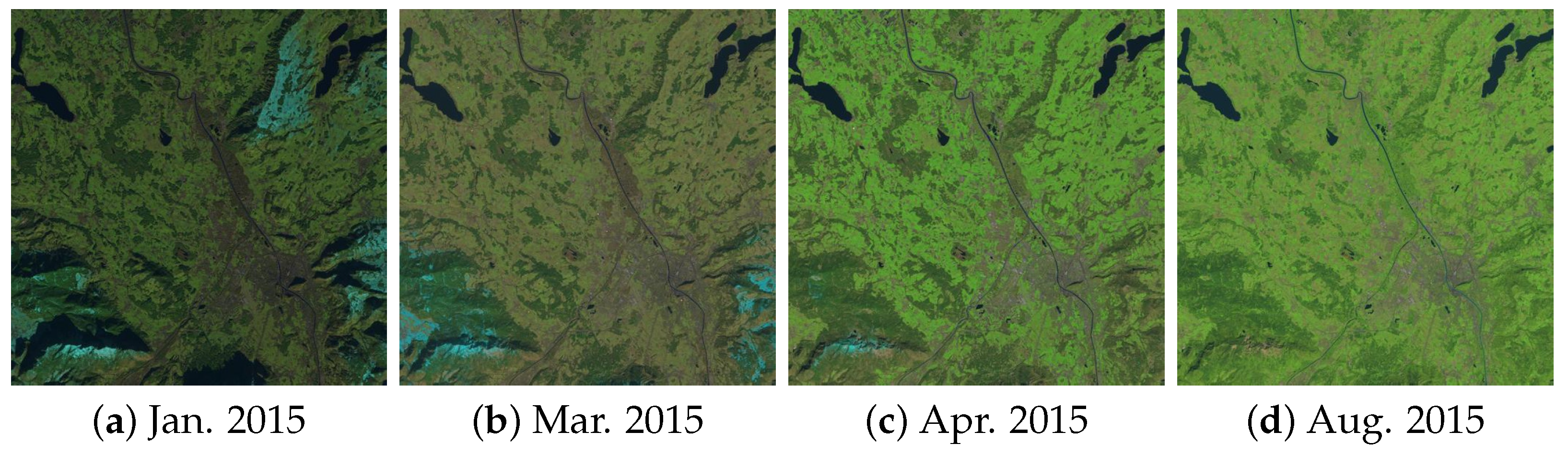
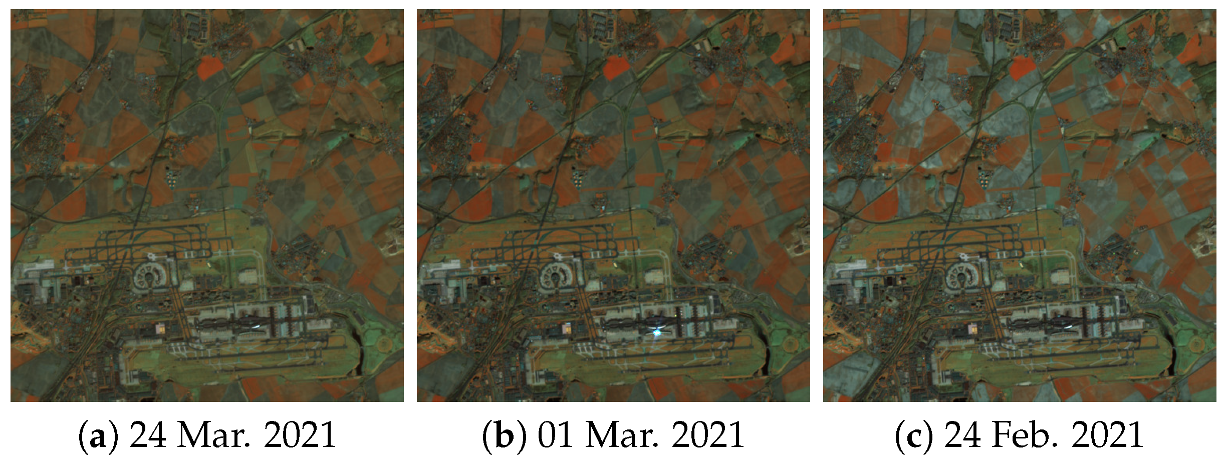
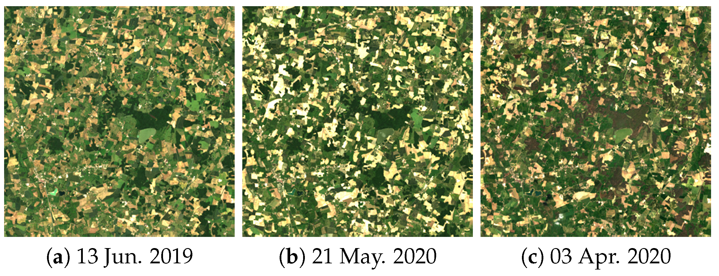
Initially, we employed multitemporal remote sensing images to showcase the efficiency of our proposed technique in restoring information hidden by cloud cover. We generated four simulated datasets—Munich, Picardie, France, and Beijing—by extracting data from the Sentinel-2 (https://earthexplorer.usgs.gov) and Landsat-8 (https://theia.cnes.fr/atdistrib/rocket/#/home) (accessed on 21 April 2024) collections. The details of these datasets are comprehensively outlined in Table 2 and visually represented in Figure 2, Figure 3, Figure 4 and Figure 5. We refer to the ground sampling distance as GSD. Various types of cloud masks were applied to these multitemporal images to augment the complexity of the task.
To rigorously assess the effectiveness of the proposed method, we employ three quantitative metrics, mean PSNR, mean CC [39], and mean SSIM [40], as established benchmarks for this type of analysis. Superior performance is indicated by higher values across these metrics. In Table 3, we provide a comprehensive quantitative comparison of our method against established methods like TNN, ALM-IPG, TVLRSDC, and BC-SLRpGS. The highest values of PSNR, CC, and SSIM are indicated in bold for clear distinction. Our method consistently surpasses the comparative methods in PSNR across all datasets. Regarding SSIM, our method displays a slight disadvantage compared to the BC-SLRpGS method in the Munich dataset and to the ALM-IPG method in the Picardie dataset, highlighting areas for further improvement.
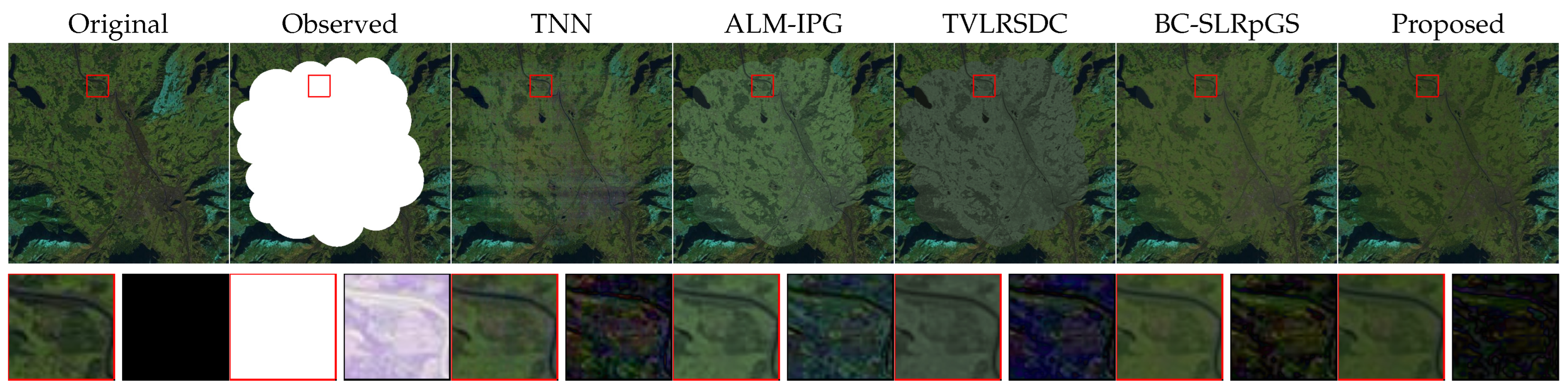
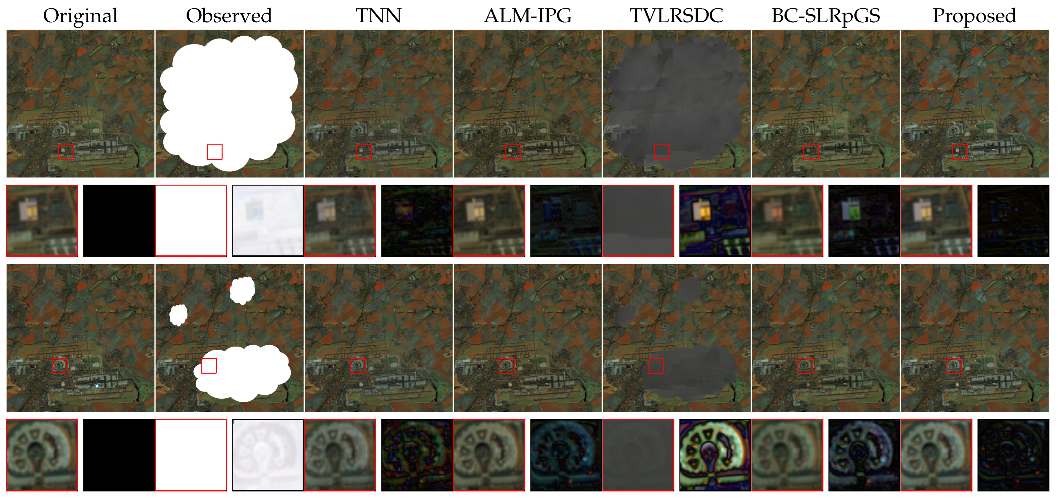
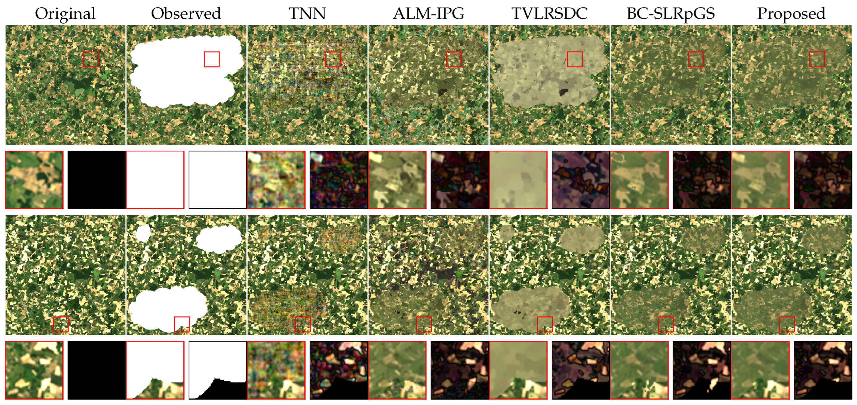
To provide a more intuitive comparison of the methods’ performance, we detail the cloud removal results in Figure 6, Figure 7, Figure 8 and Figure 9. These figures include zoomed-in patches and corresponding residual images for a more nuanced comparison. Our method and BC-SLRpGS successfully reconstructed most cloud information in the Munich dataset, whereas other methods introduced distortions in image details. In the Picardie dataset, the TVLRSDC method was unable to adequately reconstruct cloud regions, in contrast to TNN, ALM-IPG, BC-SLRpGS, and our proposed method, which yielded satisfactory results. Notably, the TNN and ALM-IPG methods necessitate a predefined cloud mask, potentially incorporating additional information into the reconstruction process. Our method produced darker residual images, as seen at the bottom of Figure 6 and Figure 7, signifying a closer similarity to cloud-free images and, thus, more effective cloud removal.
The exceptional performance of our method can be attributed to our effective utilization of the sparse structure of mode-1, -2, and -3 fibers. For the Beijing dataset, our method, along with ALM-IPG and BC-SLRpGS, achieved promising outcomes, outperforming TNN and TVLRSDC methods, which were visually inferior. The zoomed-in views in Figure 8 further substantiate our method’s clarity and precision in reconstructing more detailed and clearer images compared to other methods. For the France dataset, as illustrated in Figure 9, all tested methods failed to achieve promising results, primarily due to the dataset’s intricate details that defy reconstruction through global correlations. Nonetheless, our method yielded notably clearer outcomes compared to the others and demonstrated superior accuracy in cloud mask detection relative to BC-SLRpGS.
4.2. Real Experiments
Two real datasets, namely, the Eura and Morocco data, as outlined in Table 4 and visualized in Figure 10 and Figure 11, were used to assess the efficacy of our method. The reconstructed results for the Eura and Morocco datasets using various methods are depicted in Figure 12 and Figure 13, respectively. From Figure 12, it is evident that the TNN, ALM-IPG, and TVLRSDC methods are unsuccessful in effectively removing the clouds and reconstructing cloud information. Conversely, both BC-SLRpGS and the proposed method exhibit similar performance in this aspect. From the zoomed-in figures presented in Figure 12, it is evident that our method delivers smoother results and captures a greater amount of detail in comparison to the BC-SLRpGS method. As shown by the visual comparisons in Figure 13, our method demonstrates enhanced performance compared to the other methods. From temporal node 1 in Figure 13, the proposed method effectively eliminates the cloud, while the result of TVLRSDC still exhibits some discrete clouds. Furthermore, as displayed in the zoomed-in figure in Figure 13, our method produces a clearer reconstruction result than the other compared methods. From temporal node 2 in Figure 13, we find that the proposed method removes the cloud areas well and can preserve the cloud-free areas, whereas the TNN and ALM-IPG methods change the cloud-free information after the reconstruction process. In conclusion, the proposed method outperforms other methods in terms of both quantitative metrics and visual quality.
5. Conclusions
We have introduced a novel tri-fiber-wise sparse function to characterize the cloud component. By leveraging sparse prior information, our method excels at detecting clouds and effectively reconstructing contaminated values, providing robust results. Moreover, we described the global prior of the image component by tensor multi-rank. Utilizing the introduced novel sparse and low-rank functions, we have developed a cloud removal model that incorporates a box-constrained strategy. This model not only effectively detects clouds but also simultaneously estimates missing information. The experiments demonstrate the superior effectiveness of the proposed method to other cloud removal techniques.
Author Contributions
Conceptualization, D.-L.S. and T.-Y.J.; data curation, T.-Y.J.; formal analysis, T.-Y.J.; investigation, D.-L.S.; methodology, T.-Y.J.; resources, D.-L.S. and M.D.; software, T.-Y.J.; validation, D.-L.S. and T.-Y.J.; visualization, D.-L.S. and M.D.; writing—original draft, D.-L.S.; writing—review and editing, T.-Y.J. and M.D. All authors have read and agreed to the published version of the manuscript.
Funding
This research was funded in part by the National Natural Science Foundation of China under Grants 12001059, 12001432, 12071062, and 12201522, in part by the Natural Science Foundation of Shaanxi Province under Grant 2020JQ-342, and in part by the Fundamental Research Funds for the Central Universities under Grant 2682023CX069.
Data Availability Statement
Data are contained within the article.
Conflicts of Interest
The authors declare no conflicts of interest.
References
- Gao, L.; Wang, Z.; Zhuang, L.; Yu, H.; Zhang, B.; Chanussot, J. Using Low-Rank Representation of Abundance Maps and Nonnegative Tensor Factorization for Hyperspectral Nonlinear Unmixing. IEEE Trans. Geosci. Remote Sens. 2022, 60, 5504017. [Google Scholar] [CrossRef]
- Yao, J.; Meng, D.; Zhao, Q.; Cao, W.; Xu, Z. Nonconvex-Sparsity and Nonlocal-Smoothness-Based Blind Hyperspectral Unmixing. IEEE Trans. Image Process. 2019, 28, 2991–3006. [Google Scholar] [CrossRef] [PubMed]
- Wang, K.; Wang, Y.; Zhao, X.L.; Chan, J.C.W.; Xu, Z.; Meng, D. Hyperspectral and Multispectral Image Fusion via Nonlocal Low-Rank Tensor Decomposition and Spectral Unmixing. IEEE Trans. Geosci. Remote Sens. 2020, 58, 7654–7671. [Google Scholar] [CrossRef]
- He, W.; Yokoya, N.; Yuan, X. Fast Hyperspectral Image Recovery of Dual-Camera Compressive Hyperspectral Imaging via Non-Iterative Subspace-Based Fusion. IEEE Trans. Image Process. 2021, 30, 7170–7183. [Google Scholar] [CrossRef] [PubMed]
- Dian, R.; Li, S.; Sun, B.; Guo, A. Recent Advances and New Guidelines on Hyperspectral and Multispectral Image Fusion. Inf. Fusion 2021, 69, 40–51. [Google Scholar] [CrossRef]
- Li, J.; Zhang, Y.; Sheng, Q.; Wu, Z.; Wang, B.; Hu, Z.; Shen, G.; Schmitt, M.; Molinier, M. Thin Cloud Removal Fusing Full Spectral and Spatial Features for Sentinel-2 Imagery. IEEE J. Sel. Top. Appl. Earth Obs. Remote Sens. 2022, 15, 8759–8775. [Google Scholar] [CrossRef]
- Hong, D.; Gao, L.; Yao, J.; Zhang, B.; Plaza, A.; Chanussot, J. Graph Convolutional Networks for Hyperspectral Image Classification. IEEE Trans. Geosci. Remote Sens. 2021, 59, 5966–5978. [Google Scholar] [CrossRef]
- Cao, R.; Chen, Y.; Chen, J.; Zhu, X.; Shen, M. Thick Cloud Removal in Landsat Images based on Autoregression of Landsat Time-Series Data. Remote Sens. Environ. 2020, 249, 112001. [Google Scholar] [CrossRef]
- Xu, S.; Cao, X.; Peng, J.; Ke, Q.; Ma, C.; Meng, D. Hyperspectral Image Denoising by Asymmetric Noise Modeling. IEEE Trans. Geosci. Remote Sens. 2022, 60, 5545214. [Google Scholar] [CrossRef]
- Zheng, W.J.; Zhao, X.L.; Zheng, Y.B.; Lin, J.; Zhuang, L.; Huang, T.Z. Spatial-Spectral-Temporal Connective Tensor Network Decomposition for Thick Cloud Removal. ISPRS J. Photogramm. Remote Sens. 2023, 199, 182–194. [Google Scholar] [CrossRef]
- Chen, Y.; Chen, M.; He, W.; Zeng, J.; Huang, M.; Zheng, Y.-B. Thick Cloud Removal in Multitemporal Remote Sensing Images via Low-Rank Regularized Self-Supervised Network. IEEE Trans. Geosci. Remote Sens. 2024, 62, 5506613. [Google Scholar] [CrossRef]
- Criminisi, A.; Perez, P.; Toyama, K. Region filling and object removal by exemplar-based image inpainting. IEEE Trans. Image Process. 2004, 13, 1200–1212. [Google Scholar] [CrossRef] [PubMed]
- Shen, H.; Zhang, L. A MAP-Based Algorithm for Destriping and Inpainting of Remotely Sensed Images. IEEE Trans. Geosci. Remote Sens. 2009, 47, 1492–1502. [Google Scholar] [CrossRef]
- He, K.; Sun, J. Image Completion Approaches Using the Statistics of Similar Patches. IEEE Trans. Pattern Anal. Mach. Intell. 2014, 36, 2423–2435. [Google Scholar] [CrossRef] [PubMed]
- Mendez-Rial, R.; Calvino-Cancela, M.; Martin-Herrero, J. Anisotropic Inpainting of the Hypercube. IEEE Geosci. Remote Sens. Lett. 2012, 9, 214–218. [Google Scholar] [CrossRef]
- Wang, L.; Qu, J.; Xiong, X.; Hao, X.; Xie, Y.; Che, N. A New Method for Retrieving Band 6 of Aqua MODIS. IEEE Geosci. Remote Sens. Lett. 2006, 3, 267–270. [Google Scholar] [CrossRef]
- Li, X.; Shen, H.; Zhang, L.; Zhang, H.; Yuan, Q. Dead Pixel Completion of Aqua MODIS Band 6 Using a Robust M-Estimator Multiregression. IEEE Geosci. Remote Sens. Lett. 2014, 11, 768–772. [Google Scholar]
- Lin, C.H.; Tsai, P.H.; Lai, K.H.; Chen, J.Y. Cloud Removal from Multitemporal Satellite Images using Information Cloning. IEEE Trans. Geosci. Remote Sens. 2012, 51, 232–241. [Google Scholar] [CrossRef]
- Li, X.; Shen, H.; Li, H.; Zhang, L. Patch Matching-Based Multitemporal Group Sparse Representation for the Missing Information Reconstruction of Remote-Sensing Images. IEEE J. Sel. Top. Appl. Earth Obs. Remote Sens. 2016, 9, 3629–3641. [Google Scholar] [CrossRef]
- Wang, J.; Olsen, P.A.; Conn, A.R.; Lozano, A.C. Removing Clouds and Recovering Ground Observations in Satellite Image Sequences via Temporally Contiguous Robust Matrix Completion. In Proceedings of the IEEE Conference on Computer Vision and Pattern Recognition (CVPR), Las Vegas, NV, USA, 27–30 June 2016; pp. 2754–2763. [Google Scholar]
- Zhang, Q.; Yuan, Q.; Li, J.; Li, Z.; Shen, H.; Zhang, L. Thick Cloud and Cloud Shadow Removal in Multitemporal Imagery using Progressively Spatio-Temporal Patch Group Deep Learning. ISPRS J. Photogramm. Remote Sens. 2020, 162, 148–160. [Google Scholar] [CrossRef]
- Zhang, Q.; Yuan, Q.; Li, Z.; Sun, F.; Zhang, L. Combined Deep Prior with Low-Rank Tensor SVD for Thick Cloud Removal in Multitemporal Images. ISPRS J. Photogramm. Remote Sens. 2021, 177, 161–173. [Google Scholar] [CrossRef]
- Li, W.; Li, Y.; Chan, J.C.W. Thick Cloud Removal with Optical and SAR Imagery via Convolutional-MappingDeconvolutional Network. IEEE Trans. Geosci. Remote Sens. 2020, 58, 2865–2879. [Google Scholar] [CrossRef]
- Gao, J.; Yuan, Q.; Li, J.; Zhang, H.; Su, X. Cloud Removal with Fusion of High Resolution Optical and SAR images using Generative Adversarial Networks. Remote Sens. 2020, 12, 191. [Google Scholar] [CrossRef]
- Chen, B.; Huang, B.; Chen, L.; Xu, B. Spatially and Temporally Weighted Regression: A Novel Method to Produce Continuous Cloud-Free Landsat Imagery. IEEE Trans. Geosci. Remote Sens. 2017, 55, 27–37. [Google Scholar] [CrossRef]
- Melgani, F. Contextual Reconstruction of Cloud-contaminated Multitemporal Multispectral Images. IEEE Trans. Geosci. Remote Sens. 2006, 44, 442–455. [Google Scholar] [CrossRef]
- Wen, F.; Zhang, Y.; Gao, Z.; Ling, X. Two-Pass Robust Component Analysis for Cloud Removal in Satellite Image Sequence. IEEE Geosci. Remote Sens. Lett. 2018, 15, 1090–1094. [Google Scholar] [CrossRef]
- Chen, Y.; He, W.; Yokoya, N.; Huang, T.Z. Blind Cloud and Cloud Shadow Removal of Multitemporal Images based on Total Variation Regularized Low-Rank Sparsity Decomposition. ISPRS J. Photogramm. Remote Sens. 2019, 157, 93–107. [Google Scholar] [CrossRef]
- Meraner, A.; Ebel, P.; Zhu, X.X.; Schmitt, M. Cloud removal in Sentinel-2 imagery using a deep residual neural network and SAR-optical data fusion. ISPRS J. Photogramm. Remote Sens. 2020, 166, 333–346. [Google Scholar] [CrossRef]
- Wang, J.-L.; Zhao, X.-L.; Li, H.-C.; Cao, K.-X.; Miao, J.; Huang, T.-Z. Unsupervised Domain Factorization Network for Thick Cloud Removal of Multitemporal Remotely Sensed Images. IEEE Trans. Geosci. Remote Sens. 2023, 61, 5405912. [Google Scholar] [CrossRef]
- Duan, C.; Pan, J.; Li, R. Thick Cloud Removal of Remote Sensing Images Using Temporal Smoothness and Sparsity Regularized Tensor Optimization. Remote Sens. 2020, 12, 3446. [Google Scholar] [CrossRef]
- Ji, T.Y.; Chu, D.; Zhao, X.L.; Hong, D. A unified framework of cloud detection and removal based on low-rank and group sparse regularizations for multitemporal multispectral images. IEEE Trans. Geosci. Remote Sens. 2022, 60, 5303015. [Google Scholar] [CrossRef]
- Attouch, H.; Bolte, J.; Svaiter, B.F. Convergence of Descent Methods for Semi-Algebraic and Tame Problems: Proximal Algorithms, Forward–Backward Splitting, and Regularized Gauss–Seidel methods. Math. Program. 2013, 137, 91–129. [Google Scholar] [CrossRef]
- Wang, M.; Hong, D.; Han, Z.; Li, J.; Yao, J.; Gao, L.; Zhang, B.; Chanussot, J. Tensor Decompositions for Hyperspectral Data Processing in Remote Sensing: A comprehensive review. IEEE Geosci. Remote Sens. Mag. 2023, 11, 26–72. [Google Scholar] [CrossRef]
- Kolda, T.G.; Bader, B.W. Tensor Decompositions and Applications. SIAM Rev. 2009, 51, 455–500. [Google Scholar] [CrossRef]
- Zhang, Z.; Ely, G.; Aeron, S.; Hao, N.; Kilmer, M. Novel Methods for Multilinear Data Completion and De-noising based on Tensor-SVD. In Proceedings of the IEEE Conference on Computer Vision and Pattern Recognition (CVPR), Columbus, OH, USA, 23–28 June 2014; pp. 3842–3849. [Google Scholar]
- Zhang, Z.; Aeron, S. Exact Tensor Completion using t-SVD. IEEE Trans. Signal Process. 2017, 65, 1511–1526. [Google Scholar] [CrossRef]
- Yuan, L.; Li, C.; Mandic, D.; Cao, J.; Zhao, Q. Tensor Ring Decomposition with Rank Minimization on Latent Space: An Efficient Approach for Tensor Completion. In Proceedings of the AAAI Conference on Artificial Intelligence, Honolulu, HI, USA, 27 January–1 February 2019; Volume 33, pp. 9151–9158. [Google Scholar]
- Li, X.; Shen, H.; Zhang, L.; Zhang, H.; Yuan, Q.; Yang, G. Recovering Quantitative Remote Sensing Products Contaminated by Thick Clouds and Shadows using Multitemporal Dictionary Learning. IEEE Trans. Geosci. Remote Sens. 2014, 52, 7086–7098. [Google Scholar]
- Wang, Z.; Bovik, A.C.; Sheikh, H.R.; Simoncelli, E.P. Image Quality Assessment: From Error Visibility to Structural Similarity. IEEE Trans. Image Process. 2004, 13, 600–612. [Google Scholar] [CrossRef]
Figure 1.
(a) Observed cloud-contaminated image, (b) cloud component, (c–e) mode-1, -2, and -3 fiber-wise sparsity, i.e., the -norms of mode-1, -2, and -3 fibers from (b), respectively.
Figure 1.
(a) Observed cloud-contaminated image, (b) cloud component, (c–e) mode-1, -2, and -3 fiber-wise sparsity, i.e., the -norms of mode-1, -2, and -3 fibers from (b), respectively.

Figure 2.
Munich dataset taken by Landsat-8.

Figure 3.
Picardie dataset taken by Sentinel-2.

Figure 4.
Beijing dataset taken by Sentinel-2.

Figure 5.
France dataset taken by Landsat-8.

Figure 6.
The outcomes of cloud removal using various methods on the Munich dataset. The corresponding zoomed-in patches accompanying each image are depicted at the bottom.
Figure 6.
The outcomes of cloud removal using various methods on the Munich dataset. The corresponding zoomed-in patches accompanying each image are depicted at the bottom.

Figure 7.
The outcomes of cloud removal using various methods on the Picardie dataset. The corresponding zoomed-in patches accompanying each image are depicted at the bottom.
Figure 7.
The outcomes of cloud removal using various methods on the Picardie dataset. The corresponding zoomed-in patches accompanying each image are depicted at the bottom.

Figure 8.
The outcomes of cloud removal using various methods on the Beijing dataset. The corresponding zoomed-in patches accompanying each image are depicted at the bottom.
Figure 8.
The outcomes of cloud removal using various methods on the Beijing dataset. The corresponding zoomed-in patches accompanying each image are depicted at the bottom.

Figure 9.
The outcomes of cloud removal using various methods on the France dataset. The corresponding zoomed-in patches accompanying each image are depicted at the bottom.
Figure 9.
The outcomes of cloud removal using various methods on the France dataset. The corresponding zoomed-in patches accompanying each image are depicted at the bottom.

Figure 10.
Eure dataset taken by Sentinel-2.

Figure 11.
Morocco dataset taken by Sentinel-2.

Figure 12.
The outcomes of cloud removal using various methods on the Eure dataset. The second row in each image represents the zoomed-in details associated with the images above.
Figure 12.
The outcomes of cloud removal using various methods on the Eure dataset. The second row in each image represents the zoomed-in details associated with the images above.

Figure 13.
The outcomes of cloud removal using various methods on the Morocco dataset. The second row in each image represents the zoomed-in details associated with the images above.
Figure 13.
The outcomes of cloud removal using various methods on the Morocco dataset. The second row in each image represents the zoomed-in details associated with the images above.


Table 1.
Notation description.
| Notations | Interpretations |
|---|---|
| a, , , | scalar, vector, matrix, tensor |
| trace of , with | |
| unfolding of in its kth mode. | |
| ith mode-k fiber of | |
| rth frontal slice of | |
| reshaping of fourth-order tensor into third-order tensor | |
| difference operator in fourth mode |
Table 2.
Multitemporal remote sensing images for synthetic experiments.
| Data | Image Size | Spectral | Temporal | GSD | Source |
|---|---|---|---|---|---|
| Munich | 512 × 512 | 3 | 4 | 30 m | Landsat-8 |
| Picardie | 500 × 500 | 6 | 3 | 20 m | Sentinel-2 |
| Beijing | 256 × 256 | 6 | 4 | 20 m | Sentinel-2 |
| France | 400 × 400 | 7 | 3 | 30 m | Landsat-8 |
Table 3.
Quantitative metrics for simulated data. Highest values are emphasized in bold.
| Dataset | Index | Method | |||||
|---|---|---|---|---|---|---|---|
| Observed | TNN | ALM-IPG | TVLRSDC | BC-SLRpGS | Proposed | ||
| Munich | PSNR | 4.29 | 26.66 | 23.26 | 26.23 | 27.81 | 29.6 |
| SSIM | 0.4769 | 0.8344 | 0.8462 | 0.8385 | 0.8506 | 0.8496 | |
| CC | 0.154 | 0.8897 | 0.841 | 0.8545 | 0.9013 | 0.9184 | |
| Picardie | PSNR | 4.56 | 42.89 | 43.49 | 37.33 | 43.35 | 44.06 |
| SSIM | 0.543 | 0.987 | 0.9924 | 0.9493 | 0.9899 | 0.9918 | |
| CC | 0.0904 | 0.9397 | 0.9509 | 0.7558 | 0.9421 | 0.9514 | |
| Beijing | PSNR | 5.84 | 36.71 | 38.34 | 36.14 | 38.88 | 39.58 |
| SSIM | 0.6182 | 0.9379 | 0.9608 | 0.949 | 0.9622 | 0.9638 | |
| CC | 0.0196 | 0.9384 | 0.9646 | 0.9287 | 0.9689 | 0.9729 | |
| France | PSNR | 6.28 | 28.31 | 28.32 | 27.09 | 29.56 | 30.14 |
| SSIM | 0.6224 | 0.7947 | 0.8001 | 0.8049 | 0.8488 | 0.8536 | |
| CC | 0.2398 | 0.9603 | 0.9582 | 0.9194 | 0.9661 | 0.9697 | |
Table 4.
Multitemporal remote sensing images for real experiments.
| Data | Image Size | Spectral | Temporal | GSD | Source |
|---|---|---|---|---|---|
| Eure | 400 × 400 | 4 | 4 | 10 m | Sentinel-2 |
| Morocco | 600 × 600 | 4 | 4 | 10 m | Sentinel-2 |
Disclaimer/Publisher’s Note: The statements, opinions and data contained in all publications are solely those of the individual author(s) and contributor(s) and not of MDPI and/or the editor(s). MDPI and/or the editor(s) disclaim responsibility for any injury to people or property resulting from any ideas, methods, instructions or products referred to in the content. |
© 2024 by the authors. Licensee MDPI, Basel, Switzerland. This article is an open access article distributed under the terms and conditions of the Creative Commons Attribution (CC BY) license (https://creativecommons.org/licenses/by/4.0/).
Share and Cite
MDPI and ACS Style
Sun, D.-L.; Ji, T.-Y.; Ding, M. A New Sparse Collaborative Low-Rank Prior Knowledge Representation for Thick Cloud Removal in Remote Sensing Images. Remote Sens. 2024, 16, 1518. https://0-doi-org.brum.beds.ac.uk/10.3390/rs16091518
AMA Style
Sun D-L, Ji T-Y, Ding M. A New Sparse Collaborative Low-Rank Prior Knowledge Representation for Thick Cloud Removal in Remote Sensing Images. Remote Sensing. 2024; 16(9):1518. https://0-doi-org.brum.beds.ac.uk/10.3390/rs16091518
Chicago/Turabian StyleSun, Dong-Lin, Teng-Yu Ji, and Meng Ding. 2024. "A New Sparse Collaborative Low-Rank Prior Knowledge Representation for Thick Cloud Removal in Remote Sensing Images" Remote Sensing 16, no. 9: 1518. https://0-doi-org.brum.beds.ac.uk/10.3390/rs16091518
Note that from the first issue of 2016, this journal uses article numbers instead of page numbers. See further details here.