
Fluctuations in Refracted Star Signals Caused by the Stratospheric Internal Gravity Waves

1
Research Center for Space Optical Engineering, Harbin Institute of Technology, Harbin 150001, China
2
Optical Navigation Department, Shanghai Aerospace Control Technology Institute, Shanghai 201109, China
*
Author to whom correspondence should be addressed.
Remote Sens. 2024, 16(9), 1519; https://0-doi-org.brum.beds.ac.uk/10.3390/rs16091519
Submission received: 25 March 2024
/
Revised: 23 April 2024
/
Accepted: 23 April 2024
/
Published: 25 April 2024
Abstract
:The application of starlight refraction navigation to spacecraft and space weapons is a significant development. However, the irregular stratospheric atmosphere can cause fluctuations in relative light intensity and refraction angles of refracted stars, which need to be analyzed to provide guidance for system design and simulation verification. The internal gravity wave (IGW) is an important component of the irregular atmosphere. Based on the Rytov approximation, closed-form approximations were obtained, which can more intuitively reveal the relationship between the IGW parameters and the star signals’ statistical characteristics. From the GOMOS observations, the influence of the stratosphere from 25 km to 35 km on the fluctuations in relative intensity and refraction angles was analyzed in this study. As the height increased, the fluctuations in starlight signals gradually weakened. Compared with the numerical solution, the error of the closed-form approximations for relative intensity fluctuations was no more than 10%, and the error for refraction angle fluctuations was 1.0%. Compared with the measured data, the error of the closed-form approximations for relative intensity was 6.3%. The proposed approximations better reflect the relationship between IGW parameters and star signal fluctuations compared to the existing approximation. The research in this article can provide a reference for application assessment based on starlight refraction navigation.
1. Introduction
Under the condition of Global Navigation Satellite System (GNSS) rejection, starlight refraction navigation may be a backup method for navigation. It can provide position and altitude information for low-orbit satellites and space weapons [1], using atmospheric refraction angles at around 25 km. Based on the assumption that the atmospheric density changes exponentially with height, Robert proposed a starlight atmospheric refraction model [2]. The atmospheric refraction model assumes the refraction angle is only related to the tangent height. At a tangent height of 25 km, the ideal refraction angle is 150″. Position and altitude information can be calculated to achieve autonomous navigation with the refraction angles of starlight [3]. However, the stratosphere’s air density irregularities [4] can cause star signal fluctuations, reducing the quality of star maps and affecting navigation accuracy. The feasibility of starlight refraction navigation needs to be analyzed. Based on the Rytov approximation, the theoretical calculations of star signal fluctuations can provide a reference for the design of the navigation system and the algorithm. Analyzing the impact of the different parameters of irregular atmospheres on starlight signals can provide a basis for the verification of the system simulation.
The stratosphere exhibits anisotropic and isotropic characteristics due to internal gravity waves (IGWs) and turbulence [5]. The following three methods are commonly used to study the atmospheric characteristics of the stratosphere. One method is to study IGWs based on temperature or density measured by remote sensing satellites [6]. However, due to the measurement data’s time and space limitations, the IGW distribution in the stratosphere is often studied monthly. Therefore, the first method cannot reflect the instantaneous characteristics of IGWs. The second method is to invert the parameters of IGWs using radio sources. Due to the radio wavelength limitation, this method cannot invert the inner scale parameters of IGWs [7]. The third method is to invert the parameters of IGWs and turbulence using spectral measurement data [8], such as GOMOS data. GOMOS is an instrument that is on board the ENVISAT satellite, which uses refracted stars to study the atmosphere. GOMOS is equipped with two fast photometers sampling at a frequency of 1 kHz in the ranges 644–705 nm and 466–528 nm. The third method can be used to further study the impact of IGWs and turbulence on star signals, which is adopted in this article.
Irregular atmospheres can cause star signal fluctuations. In 2008, Robert [9] analyzed the stellar scintillation obtained from a balloon-borne spectrometer. When the exposure time was 0.42 ms, the contribution of IGWs was greater than that of turbulence in the visible band. Gurvich [10] derived the effects of turbulence and IGWs on star maps, but the influence of anisotropy was ignored. In 2008, Du [11] derived the effects of turbulence and IGWs on the star refraction angle. However, he did not consider the influence of anisotropy. In 2012, Michael E. Gorbunov [12] analyzed the influence of IGWs on radio occultation signals based on multiple-phase screens. In 2017, Yang [13] used Fluent 17.0 software to simulate the density fluctuation field of the stratosphere, and the ray tracing results showed that the starlight would be deflected due to the air density irregularities. In 2020, Kan [14] further analyzed the impact of IGWs and turbulence on radio signals. However, because the radio wavelength is much larger than that of visible light, the approximate formula obtained does not apply to visible light. In 2023, based on the refraction principle of light and ten years of atmospheric data from TIMED/SABER, Wu [15] used the ray tracing algorithm to analyze the starlight refraction angle and found that the fluctuations in the starlight refraction angle are related to IGWs in the stratosphere. However, the monthly statistical density characteristics cannot reflect the instantaneous characteristics of IGWs, which can affect the image of the star.
In general, the impact of the stratosphere on fluctuations in star signals is still unclear. Based on the GOMOS data, this article analyzed the effects of IGWs and turbulence on stellar fluctuations from 25 km to 35 km. IGWs are an important component of the irregular atmosphere. The closed-form approximations for IGW are obtained. Compared with the numerical integration solution, the closed-form approximations can more intuitively reveal the relationship between the IGW parameters and the star signals’ statistical characteristics. Section 2 introduces the characteristics of stratospheric IGWs and turbulence. Section 3 derives the closed-form approximations. Section 4 demonstrates the experimental results and analysis. This paper is concluded in Section 5. The research in this article can provide theoretical support for simulation verification and system design.
2. Spectral Model of Refractivity Fluctuation
Because stars are infinitely distant from the Earth, the starlight can be considered a plane wave. Figure 1 shows a diagram of starlight propagation from the atmosphere to the satellite. Starlight first passes through the atmosphere, and its phase distribution changes. The propagation distance of the starlight in the atmosphere is Lt. Then, the starlight propagates through a vacuum to reach the star sensors. Starlight propagates along the z-axis, the y-axis is perpendicular to the planet’s limb, and the x-axis is parallel to the limb. The “thin phase-changing screen” assumes that the atmosphere the starlight passes through is a single-phase screen [16], which is located at the oyz plane at a distance L from the satellite. The thin screen is orthogonal to the z-axis and located at the ray perigee point, and the ray perigee point is the place where the light is closest to the surface of the Earth and corresponds to the tangent height . When the low-orbit satellite height is 792 km, the distance L is ~3200 km at a tangent height of 30 km.
The anisotropic and isotropic three-dimensional spectrum for IGWs and turbulence can be expressed as follows [17]:
where, for the IGWs, is the structure characteristic defining the power of the anisotropic irregularities. is the spatial wave number. and are the wave numbers corresponding to the outer scale and the inner scale . , A = 1, and is the coefficient of anisotropy [8]. For the turbulence, is the structure characteristic for the isotropic irregularities, and is the wave number corresponding to the inner scale . , , A = 0.033, and for the turbulence [8].
Assuming the atmospheric refractivity fluctuations are locally homogeneous in a spherical layer, the two-dimensional power spectral density (PSD) of the refractivity fluctuations in the phase screen can be obtained:
where is the radius of the Earth, H is the atmospheric scale height, and is the optical path length in the atmosphere. is the refractivity at the ray perigee point. In low-latitude regions, the USSA standard atmospheric model can be used to calculate the above parameters. At a height of 30 km, the refractivity is and = 6300 m. U(a, b, z) in Equation (3) is the confluent hypergeometric function.
At the observation plane, located at a distance L from the ray perigee, the two-dimensional spectrum of relative light intensity fluctuations is related to as follows.
where the factor takes into account the diffraction of light, the refractive attenuation q, and the effects of chromatic aberration [17].
The two-dimensional PSD of relative light intensity in Equation (6) is integrated to obtain one-dimensional PSD of relative light intensity , as shown in Equation (7).
where is the wave number along the satellite trajectory on the phase screen, and is the oblique angle, as shown in Figure 2 of [17].
3. Relative Intensity and Refraction Angle Fluctuations
3.1. Relative Intensity Fluctuations
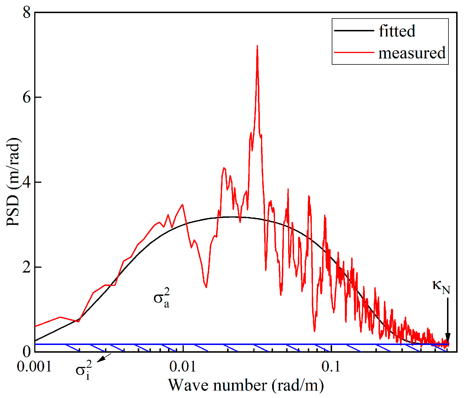
Based on the one-dimensional PSD of relative intensity and the observed scintillation data of GOMOS, the atmospheric IGWs and turbulence parameters at different tangent heights can be fitted [8]. Figure 2 shows the measured PSD and fitted PSD at (32°S, 162°E). For IGW, the corresponding inner scale is 10.3 m, the outer scale is 0.86 km, and . For turbulence, the inner scale is 0.2 m and . The stellar scintillation is caused by IGWs and turbulence. The relative intensity variance can be computed as . The spectral density of isotropic scintillation is practically constant for wave numbers . So, the blue diagonal area in Figure 2 corresponds to the relative intensity variance caused by turbulence. The other area corresponds to the relative intensity variance caused by IGWs. is the Nyquist frequency. . is the Nyquist frequency for the photometer. is the ray perigee velocity.
Based on the one-dimensional PSD of relative intensity, the variance of the relative intensity can be obtained, as shown in Equation (8).
where is the Nyquist frequency.
When the inner scale of IGWs is smaller than the Nyquist frequency , the variance of the relative intensity caused by IGWs can be obtained:
where is the two-dimensional PSD of relative intensity for IGWs.
For the condition , the 2D relative intensity fluctuation spectra on the observed surface are as follows [17]:
where q is the refractive attenuation dependent on the height. Refractive attenuation is 0.86 at a height of 30 km. , and is the wavelength of light. takes into account the averaging effect of the aperture with diameter [18]. The optical system has an aperture of 0.3 m to suppress the strong limb backgrounds [19]. is the Bessel function. The chromatic aberration . is the spectral width. is the refraction angle.
When wave number is greater than or is greater than , will rapidly decay and have a relatively small impact on intensity fluctuations. When is less than and is less than , has a great impact on intensity fluctuations. When wave number is less than , Z will satisfy Equation (12).
The function is an increasing function for Z. In addition, the confluent hypergeometric function has the following properties:
When Z equals , A is 0.55. When the condition is met, A is less than 0.6. When the condition is met, A is more than 0.6 and less than 1. A can take the average value of 0.7 as a fixed value, and the PSD of IGWs can be expressed as follows:
The variance of relative intensity caused by IGWs can be calculated using Equation (15).
When and is less than , the term in the sine portion of Equation (15) is less than 1, and is approximately 1. The variance of intensity can be obtained using the following equations:
where is approximately a fixed value at a fixed height, as is much greater than .
Based on the polar coordinate system transformation and the confluent hypergeometric function, the closed-form approximations of relative intensity fluctuations can be obtained, as shown in Equation (18).
The first term on the right side of Equation (18) is the stellar scintillation for monochromatic waves, and the second term is the effect of dispersion on scintillation. It shows that dispersion will reduce stellar scintillation. Equation (18) can be further simplified. When , is a fixed value of about 0.85, and is a fixed value of about 0.147. Equation (18) can be further simplified, as shown in Equation (21). Compared with Equation (9), which is an integral equation, Equation (21), which is an approximate equation, can more intuitively reveal the relationship between the parameters of IGWs and the relative intensity fluctuations.
where B1 and B2 are related to height. and at a height of 30 km.
Equation (21) shows that the variance of relative intensity is related to the IGW structure characteristic and inner scale. The intensity variance is proportional to and is influenced by the inner scale .
The effect of turbulence on intensity fluctuations can be calculated numerically using Equation (22). The inner scale of turbulence is approximately 0.1 to 0.5 m in the stratosphere. Normally, the inner scale of turbulence is greater than the Nyquist frequency , but this article does not provide an approximate solution for turbulence.
where is the PSD of the refractivity fluctuations for turbulence.
The intensity fluctuations caused by irregular air density in the stratosphere are
3.2. Refraction Angle Fluctuations
For monochromatic waves, the spectra of phase on the observed surface [14] are calculated using Equation (24).
The refraction angle fluctuations and in the z and y directions for the IGWs can be calculated using Equation (25).
Based on the polar coordinate system transformation and the confluent hypergeometric function, the closed-form approximations of refraction angle fluctuations can be obtained using Equations (26) and (27).
The sum variance of the refraction angle caused by IGWs is as follows:
Because the outer scale of IGWs is much larger than the inner scale, is a fixed value of about 1.3. Equation (28) can be further simplified, as shown in Equation (29). Compared with Equation (25), which is an integral equation, Equation (29), which is an approximate equation, can more intuitively reveal the relationship between the parameters of IGWs and the refraction angle fluctuations.
Equations (26) and (27) show that the refraction angle fluctuation in the z-direction is much greater than that in the y-direction, which is caused by the anisotropy of IGWs. Moreover, the fluctuation of the refraction angle is mainly determined by the outer scale of IGWs.
The effect of turbulence on the refraction fluctuations can be calculated numerically using Equation (30). The Nyquist frequency is not considered here because the refraction angle of the infinite interval, which is caused by turbulence, is very small, as shown in the next section.
The refraction angle fluctuations caused by irregular air density in the stratosphere are
4. Experimental Results and Analysis
4.1. Experimental Dataset
The scintillation measurements taken by the GOMOS red photometer were used to retrieve the parameters of the IGWs and turbulence. In low-latitude regions, atmospheric density fluctuates less, and high-precision navigation can be performed. Ten occultation events were analyzed in low-latitude regions, as shown in Table 1. The occultation information (at 25 km) is shown in Table 1. This article analyzed the impact of the stratosphere from 25 km to 35 km on star signals. is the oblique angle.
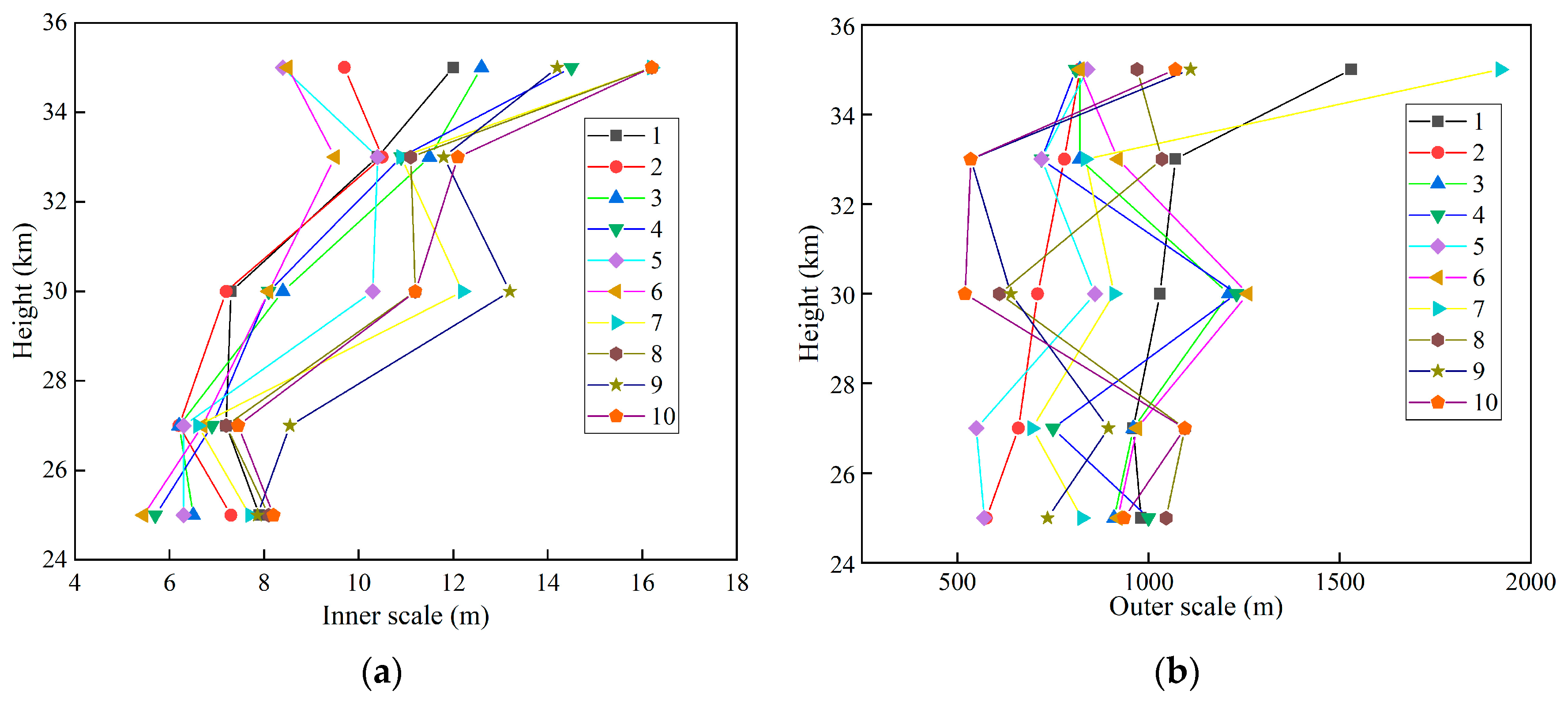
Based on the measured data of GOMOS and the fit method [8], the atmospheric IGWs and turbulence parameters at different tangent heights were fitted. It is impossible to retrieve the turbulence inner scale from the GOMOS scintillations due to limited sampling frequency, and the turbulence inner scale is approximately 0.1 to 0.5 m in the stratosphere [20]. The turbulence inner scale is assumed to be 0.2 m based on the measured data.
The fitted parameters are shown in Figure 3 and Figure 4. In ten observations, the parameters were obtained at different tangent heights. The structure characteristic CW is nearly constant with height. The turbulent structure characteristic CK grows with height, with an especially rapid increase at heights of 25–35 km. The average structure characteristic CW of the result is 4.7 × 10⁻¹¹ m−2. Furthermore, the average structure characteristic CW of the USSA standard atmosphere model is about 5 × 10⁻¹¹ m−2.
To evaluate the accuracy of the fitted parameters for IGWs and turbulence, these parameters were substituted into Equations (2), (6), (8), and (23) to numerically calculate the intensity fluctuation . Moreover, was compared with the measured intensity fluctuation to indirectly evaluate the accuracy of the overall fitting parameters as follows.
where N = 5, which corresponds to different heights. is the average intensity fluctuation for ten observations.
To evaluate the error of the closed-form approximation with the numerical solution, these fitted parameters were substituted into Equations (21) and (29) to obtain the approximate relative intensity fluctuation and the refraction angle fluctuation . These fitted parameters were substituted into Equations (2), (9), and (25) to numerically calculate the intensity fluctuation and the refraction angle fluctuation . The error of the closed-form approximation with the numerical solution is defined as follows:
To evaluate the error of the closed-form approximation with the measured data, the error of the closed-form approximation with the measured data is defined using Equation (34). The measured data were obtained by subtracting the corresponding turbulence scintillation from the measured stellar scintillation . is the numerical scintillation of turbulence.
4.2. Results and Analysis
4.2.1. Relative Intensity Fluctuations
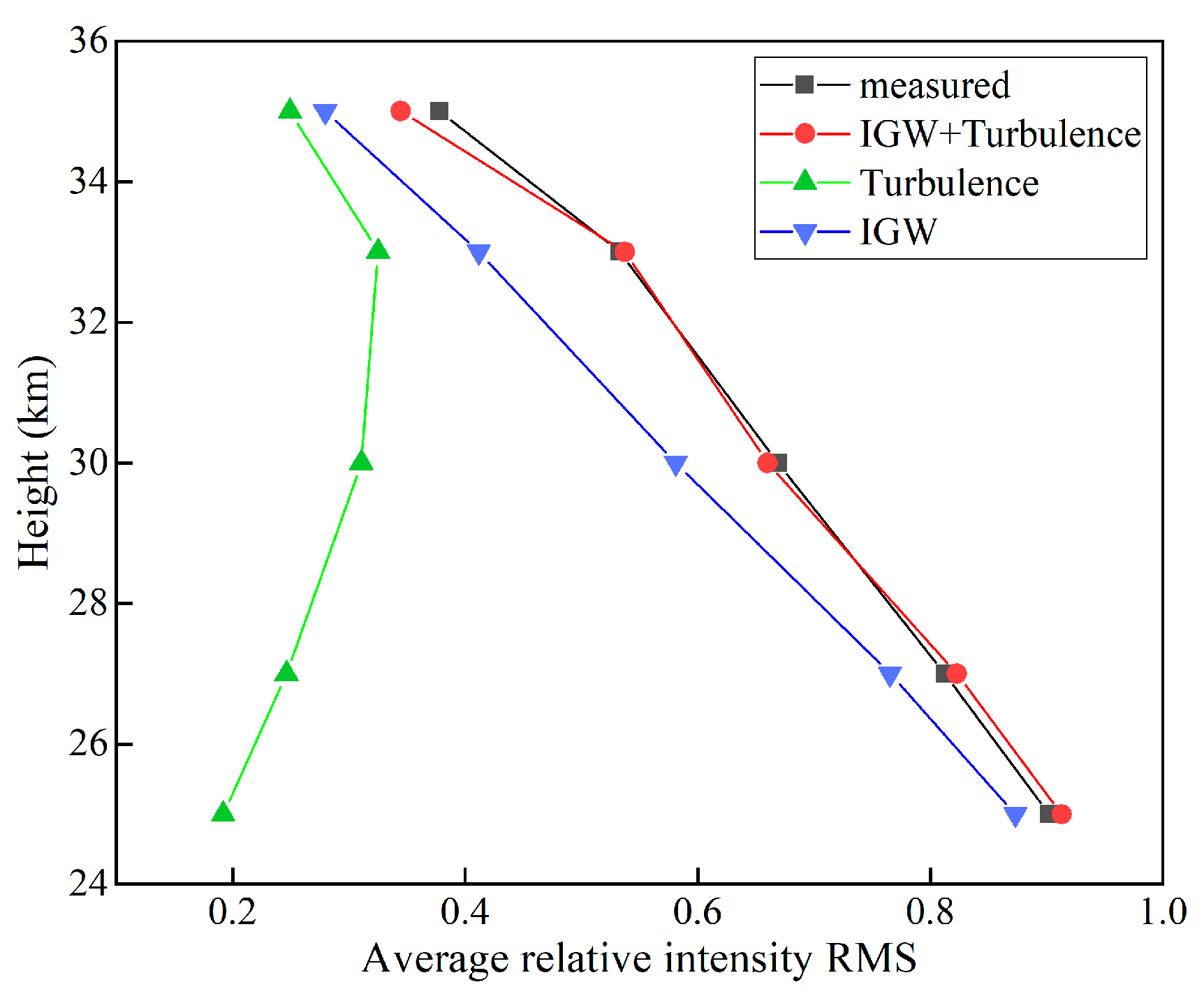
Based on the fitted parameters and Equations (2), (6), and (23), the relative intensity fluctuations caused by IGWs and turbulence can be obtained numerically. The average intensity root mean square (RMS) is shown in Figure 5. It can be seen that as the height increases, the relative intensity fluctuations gradually decrease. The average relative intensity fluctuations were calculated numerically. The measured data are from the GOMOS data. The relative intensity fluctuation obtained using numerical calculation is consistent with the measured data. Based on Equation (32), the accuracy index is 96.4%, which indirectly reflects the fitted parameters’ accuracy. Figure 5 also shows the average relative intensity fluctuation caused by turbulence.
To evaluate the error of the closed-form approximation with the measured data and numerical solution, Figure 6 shows the average intensity fluctuations calculated via the closed-form approximation, the numerical solution, and the measured data using solid lines. The figure also uses dashed lines to show the intensity fluctuations caused by IGWs from different observations. Based on Equation (34), the error of the closed-form approximation is 6.3% with the measured data. The error of the closed-form approximation is 7.3% with the numerical solution. As the height increases, the relative intensity fluctuations gradually decrease, and these fluctuations are proportional to density and influenced by internal scales.
The IGW parameters (occultation event 5) in Figure 2 were used to analyze the influence of the inner scale on scintillation. Moreover, the proposed approximation was compared with the approximation of Kan et al. [14]. The latter was derived in the radio band. The result is shown in Figure 7. As the inner scale increases, the stellar scintillation decreases, consistent with Equation (21). The error between the proposed approximation and the numerical results does not exceed 10%, but the error of Kan’s approximation is 50.4%. The wavelength of radio waves is longer than visible light, and its corresponding Fresnel scale is far larger than the inner scale of IGWs. The influence of the inner scale on radio scintillation can be ignored. However, in the visible light range, the Fresnel scale is about a few meters, and the inner scale must be considered. Therefore, the approximation of Kan does not apply to the visible light band.
4.2.2. Refraction Angle Fluctuations
Based on the fitted parameters and Equations (2), (25), and (30), the refraction angle fluctuations caused by IGWs and turbulence can be obtained numerically. The average refraction angle fluctuations caused by the stratosphere in different observations were calculated, as shown in Figure 8. The refraction angle fluctuations caused by the IGWs from different observations are shown in Figure 9. It can be seen that as the height increases, the refraction angle fluctuations gradually decrease. The results of the numerical calculations are consistent with the conclusions obtained from the closed-form approximation (26). The error of the closed-form approximation is 0.7% with the numerical solution. Based on different observations, the refraction angle fluctuation caused by turbulence is less than 0.1″, which is much smaller than that caused by IGWs.
At a height of 30 km, the refraction angle is approximately 67″ based on the standard atmosphere. The refraction angle RMS is 0.74″ at a latitude of 35°S in Figure 9, representing a density fluctuation of approximately 1.1% in the stratosphere [21] based on geometric optics. Based on the monthly statistical methods in reference [15] and the TIMED/SABER atmospheric density data from 2002, the fluctuation of atmospheric density is 2.15% at a latitude of 35°S. It may indicate that the IGWs obtained from GOMOS are small-scale, which reflects the instantaneous characteristics of IGWs.
The IGW parameters in Figure 2 were used to analyze the influence of the outer scale on the refraction angle. The proposed approximation was compared with the approximation of Kan. The result is shown in Figure 10. Whether in the radio band or the visible light band, the refraction angle is influenced by the outer scales. The changing trend of the proposed approximations is consistent with that of Kan’s approximation, and both reveal that the refraction angle is proportional to . The maximum error between the proposed approximation and the numerical results is 4.47%. Based on Equation (33), the mean error of the proposed approximation does not exceed 1%, but the mean error of Kan’s approximation is 30.1% because the approximations of Kan are derived from the radio band. The approximations proposed in this paper can better reveal the influence of various parameters on the refraction angle, providing good guidance for subsequent navigation simulations.
The error of the closed-form approximations regarding the relative intensity fluctuation and the refraction angle fluctuation compared with the numerical solution is shown in Table 2. Compared with the measured data, the error of the closed-form approximations for relative intensity is 6.3%. It can be seen that the error of star signal fluctuation obtained using the closed-form approximations is far less than that of the existing approximations.
4.2.3. Other Parameter Analysis
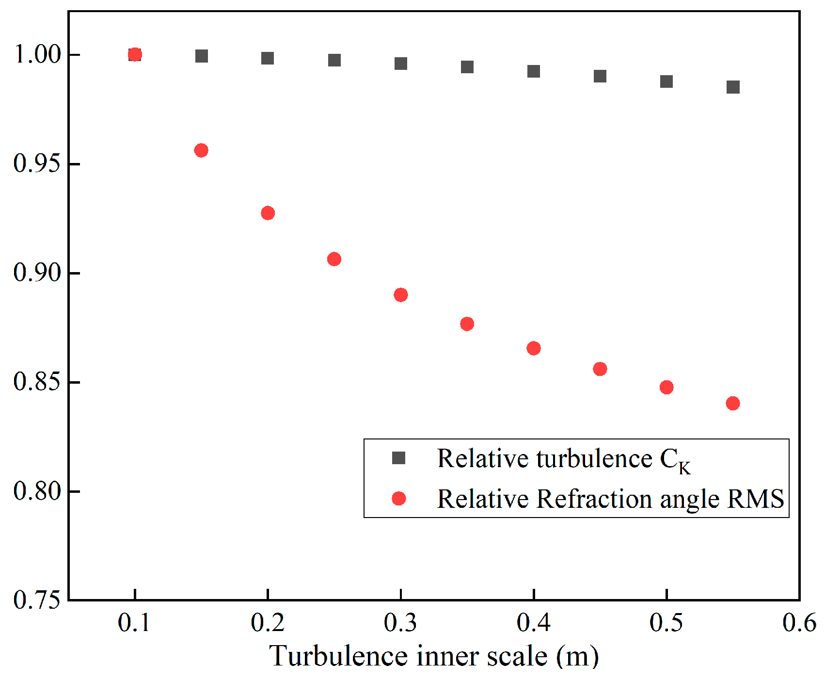
In this article, it is assumed that the inner scale of turbulence is 0.2 m. Using numerical simulation, the effects of different inner scales on turbulence parameters, scintillation, and refraction angles were analyzed, as shown in Figure 11. These data have been normalized separately based on the maximum value. Using numerical calculations, it was found that within the turbulent internal scale range of 0.1–0.5 m, the variation in CK does not exceed 3%, and the impact on relative intensity does not exceed 0.03%. Although the variation in the refraction angle is about 15%, the refraction angle fluctuation caused by turbulence is still very small. Within the range of 0.1–0.5 m, the impact of different inner scales on star fluctuation is not significantly different. Therefore, the inner scale of 0.2 m was chosen.
5. Conclusions
In order to study the irregular stratospheric air density effects on star signal fluctuations, the influence of the stratosphere from 25 km to 35 km on the fluctuations in star intensity and refraction angles was analyzed. Compared to existing approximate formulas, the closed-form approximations can more intuitively reveal the relationships between the IGW parameters and the statistical characteristics of the star signals. The research in this article can provide a valuable reference for an application assessment based on starlight refraction navigation. The calculations in this article are based on the Rytov assumption. When the height is less than 27 km, strong scintillation is encountered in some occultation events. In this case, the inversion formula and the related conclusions in this article are no longer applicable. Moreover, the stratosphere will be analyzed using strong scintillation theory in the future.
Author Contributions
Methodology, S.W.; funding acquisition, X.Z.; writing—review and editing, H.W.; formal analysis, Z.Y. All authors have read and agreed to the published version of the manuscript.
Funding
This research was supported by the National Key Research and Development Program of China, grant number 2019YFA0706003.
Data Availability Statement
Data are contained within the article.
Conflicts of Interest
The authors declare no conflicts of interest.
References
- Wang, H.; Wu, S.; Wang, B.; Yan, Z.; Yao, S.; Zeliu, C. Near-infrared Star Map Simulation for Starlight Refraction Sensor based on Ray Tracing. Infrared Phys. Technol. 2023, 132, 104760. [Google Scholar] [CrossRef]
- White, R.L.; Thurman, S.W.; Barnes, F.A. Autonomous Satellite Navigation Using Observations of Starlight Atmospheric Refraction. Navigation 1985, 32, 317–333. [Google Scholar] [CrossRef]
- Fan, S.; Yan, Z.; Lin, Y. Adaptively tuning sampling weights of the unscented Kalman filter in starlight refraction navigation. Optik 2017, 148, 300–311. [Google Scholar]
- Bi, C.; Qing, C.; Wu, P.; Jin, X.; Liu, Q.; Qian, X.; Weng, N. Optical turbulence profile in marine environment with artificial neural network model. Remote Sens. 2022, 14, 2267. [Google Scholar] [CrossRef]
- Grechko, G.M.; Gurvich, A.S.; Kan, V.; Kireev, S.V.; Savchenko, S.A. Anisotropy of spatial structures in the middle atmosphere. Adv. Space Res. 1992, 12, 169–175. [Google Scholar] [CrossRef]
- Cheng, X.; Yang, J.; Xiao, C.; Hu, X. Density Correction of NRLMSISE-00 in the Middle Atmosphere (20–100 km) based on TIMED/SABER Density Data. Atmosphere 2020, 11, 341. [Google Scholar] [CrossRef]
- Gorbunov, M.; Kan, V. The Study of Internal Gravity Waves in the Earth’s Atmosphere by Radio Occultations: A Review. Remote Sens. 2024, 16, 221. [Google Scholar] [CrossRef]
- Sofieva, V.F.; Gurvich, A.S.; Dalaudier, F.; Kan, V. Reconstruction of internal gravity wave and turbulence parameters in the stratosphere using GOMOS scintillation measurements. J. Geophys. Res. Atmos. 2007, 112, 1–14. [Google Scholar] [CrossRef]
- Robert, C.; Conan, J.M.; Michau, V.; Renard, J.B.; Robert, C.; Dalaudier, F. Retrieving parameters of the anisotropic refractive index fluctuations spectrum in the stratosphere from balloon-borne observations of stellar scintillation. J. Opt. Soc. Am. A 2008, 25, 379–393. [Google Scholar] [CrossRef] [PubMed]
- Gurvich, A.S.; Belen’kii, M.S. Influence of stratospheric turbulence on infrared imaging. J. Opt. Soc. Am. A 1995, 12, 2517–2522. [Google Scholar] [CrossRef]
- Du Wenhe, Z.Z.; Daosen, L.; Chengjiang, C.; Rui, L.; Guangyu, Z.; Yuqiang, Y. Effect of non-Kolmogorov turbulence on fluctuations in angle of arrival of starlight. Infrared Laser Eng. 2013, 42, 2779–2783. [Google Scholar]
- Gorbunov, M.E.; Kirchengast, G. Influence of anisotropic turbulence on X/K band radio occultation signals and related transmission retrieval quality. In Prodex-CN1 Task 2.2 Report to ESA/ESTEC-Draft Version; University of Graz: Graz, Austria, 2007. [Google Scholar]
- Yang, B.; Zhu, X.Y. Influence of Atmospheric Turbulence on Starlight Transmission during Satellite Celestial Navigation in Stratosphere. Yuhang Xuebao J. Astronaut. 2017, 38, 359–366. [Google Scholar]
- Kan, V.; Gorbunov, M.E.; Sofieva, V.F. Fluctuations of radio occultation signals in sounding the Earth’s atmosphere. Atmos. Meas. Tech. 2018, 11, 663–680. [Google Scholar] [CrossRef]
- Wu, S.; Wang, H.; Wang, B. Construction of a backpropagation starlight atmospheric refraction model based on ray tracing. Appl. Opt. 2023, 62, 3778–3787. [Google Scholar] [CrossRef] [PubMed]
- Salpeter, E.E. Interplanetary scintillations. I. Theory. Astrophys. J. 1967, 147, 433. [Google Scholar] [CrossRef]
- Gurvich, A.S.; Brekhovskikh, V.L. Study of the turbulence and inner waves in the stratosphere based on the observations of stellar scintillations from space: A model of scintillation spectra. Waves Random Media 2001, 11, 163–181. [Google Scholar] [CrossRef]
- Bertaux, J.L.; Kyrölä, E.; Fussen, D.; Hauchecorne, A.; Dalaudier, F.; Sofieva, V.; Tamminen, J.; Vanhellemont, F.; Fanton d’Andon, O.; Barrot, G.; et al. Global ozone monitoring by occultation of stars: An overview of GOMOS measurements on ENVISAT. Atmos. Chem. Phys. 2010, 10, 12091–12148. [Google Scholar] [CrossRef]
- Wu, S.; Wang, H.; Yan, Z. Optical system design method of the all-day starlight refraction navigation system. J. Eur. Opt. Soc.-Rapid Publ. 2023, 19, 43. [Google Scholar] [CrossRef]
- Gurvich, A.S.; Kan, V. Structure of air density irregularities in the stratosphere from spacecraft observations of stellar scintillation: 2. Characteristic scales, structure characteristics, and kinetic energy dissipation. Izv. Atmos. Ocean. Phys. 2003, 39, 311–321. [Google Scholar]
- Gounley, R.; White, R.L.; Gai, E. Autonomous satellite navigation by stellar refraction. J. Guid. Control. Dyn. 1984, 7, 129–134. [Google Scholar] [CrossRef]
Figure 1.
The thin phase screen for starlight propagation.

Figure 2.
Power spectral density of relative light intensity at a height 30 km.

Figure 3.
Turbulence and IGW structure parameters from different observations. (a) Turbulence structure parameters CK. (b) IGW structure parameters CW.
Figure 3.
Turbulence and IGW structure parameters from different observations. (a) Turbulence structure parameters CK. (b) IGW structure parameters CW.

Figure 4.
IGW inner and outer scales from different observations. (a) Inner scale lW of IGW. (b) Outer scale L0 of IGW.
Figure 4.
IGW inner and outer scales from different observations. (a) Inner scale lW of IGW. (b) Outer scale L0 of IGW.

Figure 5.
Average relative intensity RMS of measured data and numerical solution.

Figure 6.
Relative intensity RMS caused by IGWs calculated using different methods.

Figure 7.
The influence of IGW inner scale on stellar scintillation.

Figure 8.
Average refraction angle RMS of numerical solution and approximation.

Figure 9.
Refraction angle RMS caused by IGWs using numerical solution.

Figure 10.
The influence of IGW outer scale on refraction angle RMS.

Figure 11.
The influence of the inner scale of turbulence on star fluctuations.


Table 1.
Characteristics of the occultation in 2002.
| Num | Orbit | Star | α, ° | Tangent Point | Time | Vs, km/s |
|---|---|---|---|---|---|---|
| 1 | 2908 | 9Alp CMa | 67.1 | 35°S, 105°W | 20 September | 4.3 |
| 2 | 2911 | 9Alp CMa | 67.4 | 35°S, 179°E | 20 September | 4.3 |
| 3 | 2914 | 9Alp CMa | 67.4 | 33°S, 104°E | 20 September | 4.3 |
| 4 | 2915 | 9Alp CMa | 67.4 | 33°S, 179°E | 20 September | 4.3 |
| 5 | 2926 | 9Alp CMa | 68.0 | 32°S, 162°E | 21 September | 4.4 |
| 6 | 2928 | 9Alp CMa | 68.1 | 32°S, 111°E | 21 September | 4.3 |
| 7 | 3059 | Alp Eri | 28.4 | 26°N, 50°E | 30 September | 2.7 |
| 8 | 3060 | Alp Eri | 28.3 | 26°N, 26°E | 30 September | 2.7 |
| 9 | 3067 | Alp Eri | 28.1 | 26°N, 150°W | 1 October | 2.6 |
| 10 | 3077 | Alp Eri | 27.4 | 26°N, 42°W | 1 October | 2.6 |
Table 2.
The error of closed-form approximations compared with numerical solution.
| Proposed Approximation | Approximation of Kan | |
|---|---|---|
| Intensity fluctuation | 7.3% | 50.4% |
| Refraction angle fluctuation | 1.0% | 30.1% |
Disclaimer/Publisher’s Note: The statements, opinions and data contained in all publications are solely those of the individual author(s) and contributor(s) and not of MDPI and/or the editor(s). MDPI and/or the editor(s) disclaim responsibility for any injury to people or property resulting from any ideas, methods, instructions or products referred to in the content. |
© 2024 by the authors. Licensee MDPI, Basel, Switzerland. This article is an open access article distributed under the terms and conditions of the Creative Commons Attribution (CC BY) license (https://creativecommons.org/licenses/by/4.0/).
Share and Cite
MDPI and ACS Style
Wu, S.; Wang, H.; Zheng, X.; Yan, Z. Fluctuations in Refracted Star Signals Caused by the Stratospheric Internal Gravity Waves. Remote Sens. 2024, 16, 1519. https://0-doi-org.brum.beds.ac.uk/10.3390/rs16091519
AMA Style
Wu S, Wang H, Zheng X, Yan Z. Fluctuations in Refracted Star Signals Caused by the Stratospheric Internal Gravity Waves. Remote Sensing. 2024; 16(9):1519. https://0-doi-org.brum.beds.ac.uk/10.3390/rs16091519
Chicago/Turabian StyleWu, Shaochong, Hongyuan Wang, Xunjiang Zheng, and Zhiqiang Yan. 2024. "Fluctuations in Refracted Star Signals Caused by the Stratospheric Internal Gravity Waves" Remote Sensing 16, no. 9: 1519. https://0-doi-org.brum.beds.ac.uk/10.3390/rs16091519
Note that from the first issue of 2016, this journal uses article numbers instead of page numbers. See further details here.