


Speckle Noise Reduction via Linewidth Broadening for Planetary Laser Reflectance Spectrometers

NASA Goddard Space Flight Center, Greenbelt, MD 20771, USA
*
Author to whom correspondence should be addressed.
Remote Sens. 2024, 16(9), 1515; https://0-doi-org.brum.beds.ac.uk/10.3390/rs16091515
Submission received: 30 March 2024
/
Revised: 22 April 2024
/
Accepted: 23 April 2024
/
Published: 25 April 2024
(This article belongs to the Special Issue Hyperspectral Imaging and LiDAR Scanning Technology Development and Applications)
Abstract
:The low obliquity of the Moon leads to challenging solar illumination conditions at the poles, especially for passive reflectance measurements aimed at determining the presence and extent of surface volatiles. A nascent alternate method is to use active laser illumination sources in either a multispectral or hyperspectral design. With a laser spectral source, however, the achievable reflectance precision may be limited by speckle noise resulting from the interference effects of a coherent beam interacting with a rough surface. Here, we have experimentally tested the use of laser linewidth broadening to reduce speckle noise and, thus, increase reflectance precision. We performed a series of speckle imaging tests with near-infrared laser sources of varying coherence, compared them to both theory and speckle pattern simulations, and measured the reflectance precision using calibrated targets. By increasing the laser linewidth, we observed a reduction in speckle contrast and the corresponding increase in reflectance precision, which was 80% of the theoretical improvement. Finally, we discuss methods of laser linewidth broadening and spectral resolution requirements for planetary laser reflectance spectrometers.

1. Introduction
Reflectance spectroscopy has been a transformative technique for the remote study of planetary bodies, beginning with early ground-based studies of the lunar nearside and of Mars [1,2], followed by the Clementine mission to the Moon, which carried several multiband cameras which enabled the first studies of lunar far-side mineralogy [3]. Multiband imagers, hyperspectral imagers, and point and imaging spectrometers have followed in the intervening decades, which rely on the Sun as the illumination source (i.e., passive spectroscopy). The exploration and scientific focal points of international space agencies and private commercial entities have narrowed in on the lunar South Polar region [4] due to in situ resource potential primarily around water and hydroxyl (H2O/OH) [5,6,7,8,9], proximity to the epoch-defining South Pole-Aitkin Basin (SPA) [10,11], and select regions of near-constant solar illumination and Earth visibility for power and communications needs [12,13,14]. The low obliquity of the Moon means that the south pole region sees solar illumination at glancing incidence angles, and the permanently shadowed regions see no direct sunlight, only secondary illumination from crater rims. These illumination conditions present significant difficulties for passive reflectance spectroscopy measurements in this region, which motivates the use of lasers as illumination sources [15].
For lunar applications, the primary laser-based spectroscopy techniques of interest are Raman spectroscopy (in a standoff geometry) and laser reflectance spectroscopy, which would target mineralogical features and identification and qualification of volatile species such as H2O/OH [16,17,18,19,20]. Here, we will focus on laser reflectance spectroscopy, which uses precisely selected laser sources to interrogate spectral features, primarily in the near- and mid-infrared portions of the spectrum. Reflectance data from the Lunar Orbiter Laser Altimeter (LOLA) on the Lunar Reconnaissance Orbiter (LRO) were used to identify anomalously high reflectance regions at 1064 nm coincident with regions of permanent shadow that may indicate water ice exposures [6,21,22,23], but the spatial resolution and precision of the LOLA reflectance measurements were limited partly due to the laser wavelength, which was primarily designed for altimetry measurements. Higher-precision and higher-resolution laser reflectance measurements at carefully selected laser wavelengths in the mid-infrared could quantify H2O/OH abundance at the tens of ppm level [24] but will require high signal-to-noise ratios (SNR) of both the transmitted and received laser energy measurements.
A key limitation to the received energy SNR is speckle noise stemming from the interaction of the coherent laser light with the rough lunar surface [25,26]. Speckle noise becomes more severe in the mid-infrared as the speckle cell size is proportional to the laser wavelength. Speckle noise can be reduced using pulse averaging only if the laser spot is moved on the surface by ½ the laser spot size. However, this limits the laser pulse rate and reduces the achievable spatial resolution of the measurements. Speckle reduction using partially coherent sources or multiple distinct laser modules with different wavelengths has been reported for laser projection and holographic displays [27,28,29,30,31]. Particular attention has been paid to reducing speckle for green-light sources [32,33], as traditionally green laser light is produced with narrow-linewidth second harmonic generation. Speckle noise was identified as a concern in atmospheric Integrated Path Differential Absorption (IPDA) lidar measurements, but since single-frequency operation is integral to the method, spatial averaging and a loss of spatial resolution are accepted in airborne and spaceborne approaches [26,34,35,36,37]. We have not found reports of using laser linewidth broadening for high-precision reflectance measurements in the infrared. Reducing speckle noise by broadening the laser linewidth in a lunar laser reflectance spectrometer would improve the spatial resolution achievable at a given H2O/OH abundance precision or increase the H2O/OH abundance precision at a given spatial resolution, both of which are key to lunar science and exploration goals [4].
Here, we experimentally verify the use of laser linewidth broadening to increase measurement precision for infrared laser reflectance measurements using a suite of illumination sources, known-reflectance targets, and a fixed imaging geometry. We examine speckle patterns under various linewidth levels and quantify the speckle contrast in comparison with both theory and simulation. We also measured the reflectance precision as a linewidth function with the goal of optimizing the laser architecture for lunar laser spectrometers.
2. Materials and Methods
2.1. Laser and Illumination Sources
We used four laser sources and one white-light source to test the effects of temporal coherence (i.e., linewidth) on speckle contrast and reflectance precision. To ensure identical imaging conditions throughout the tests, all the laser sources were fiber optically coupled using single-mode fiber. We selected laser sources in the near-infrared (~1 µm) due to the availability of a range of linewidths and the presence of many important mineralogical and volatile spectral features in that spectral region. The results here should apply to other laser wavelengths as well. The parameters of the illumination sources used in these tests are given in Table 1.
Two of the sources, the single-frequency diode and the white light source, were chosen to assess the end member speckle states and were not analyzed as part of the linewidth comparison study. The single-frequency diode images were entirely spatial-speckle limited, while the white light images had neither spatial speckle nor temporal speckle effects and, thus, captured the contrast and reflectance precision of the imaging setup. The spectra of the remaining three sources that were used for the quantitative speckle comparisons are shown in Figure 1. The spectra were obtained using a Thorlabs Fourier Spectrum Optical Spectrum Analyzer operated in high-resolution mode with a resolution of 16 pm. Each laser was operated in continuous-wave mode for the duration of all tests.
2.2. Speckle Imaging Tests
Our speckle imaging system consisted of a fiber-coupled reflective collimator to create a collimated illumination source, a series of calibrated Spectralon reflectance standards as the targets, and a CMOS camera coupled with a 25 mm focal length, F/16 lens. The reflective collimator coupled with the single-mode fiber created a 6 mm diameter beam on the Spectralon targets. We used three Spectralon reflectance standards with specified 50, 75, and 99% 8-degree hemispherical reflectance values. At the laser wavelengths specifically, the calibrated reflectance values were 53, 80, and 99%. We used a Basler ACA2500-14gm monochrome CMOS camera with a 2.2-µm pixel pitch and a 2592 × 1944-pixel resolution. This resulted in an angular instantaneous field-of-view (IFOV) of 88 µrad and a field of view (FOV) of 228 × 171 mrad (13 × 9.8 degrees). The target was placed 200 mm from the camera, enabling capture of the entire Spectralon target within the field of view. The reflective collimator was placed adjacent to but behind the camera to lower the incidence angle onto the target. The incident angle was 15 degrees, while the emission angle to the camera was 0 degrees. The experimental setup and a representative image of the target using a white light source are shown in Figure 2.
The f-number of the lens was purposely increased to the greatest extent possible to induce a high speckle condition in the narrow linewidth limit. This enabled us to potentially observe a reduction in contrast as temporal speckle effects began to dominate with increased linewidth broadening. In a low-spatial-speckle condition, the effects of temporal speckle would not be visible due to the already low contrast.
For each illumination source, five images were captured with each of the three Spectralon targets. First, a background image was captured with the illumination source off to measure the ambient light and sensor noise. Each target was imaged in four different rotation states corresponding to 90-degree rotations about the optical axis between images. This effectively made each rotation a separate speckle experiment, which enabled us to assess the limited statistical effects of the temporal coherence on the speckle patterns. For each imaging condition (source and target combination), the camera integration time was adjusted to keep the highest pixel count near 75% of the saturation value.
Each image was processed identically in the following manner. First, a background image (laser illumination off) was subtracted from the image to remove the effects of ambient light and bad pixels. Then, we calculated the centroid of each image after applying a 100-pixel Gaussian blur to remove the effects of the speckle on the centroid. Then, a 10 × 10-mrad (57 × 57 pixels) region of interest (ROI) was selected centered at the centroid location. Within this ROI, the intensity average and standard deviation were calculated for each image. The speckle contrast in percent was calculated by dividing the standard deviation by the average and multiplying by 100 [25,32]. Only a single image was taken for each speckle pattern, but we tested the repeatability of the speckle contrast calculation in a separate experiment by taking five images at each rotation. Across each five-image set, the speckle contrast was consistent with less than 0.1% standard deviation.
Using the three reflectance standards, we also calculated the relative reflectance precision for each source using the ROI defined above. The reflectance was calculated for each image by dividing the average value in the ROI by the camera integration time. The reflectance values for the 50% and 75% reflectance targets were normalized to the 99% reflective target for each illumination source. Thus, the average reflectance for each laser source at the 99% reflective target is fixed at 0.99; however, the standard deviation is still representative of the reflectance precision.
2.3. Speckle Pattern Simulations
To simulate the speckle images at the focal plane of the camera, we used the method of propagation using Fast Fourier Transformations (FFT) [38]. Briefly, a single transverse mode is assumed and propagated through free space, which interacts with a surface that introduces phase noise into the electromagnetic field associated with the roughness of the surface.
The surface model used in these simulations is based on height displacements defined as a 2D discrete Fourier transform, with Fourier coefficients defined as:
where S(f) is the spectral density function of the surface, ζ1 is a random variable from a normal distribution with a mean of zero, and ζ2 is a random variable from a uniform distribution with limits of 0 and 2π. To simulate the spectral density function of the surface, an exponential auto-covariance model was utilized and defined as:
where σ is the rms surface roughness (0.5 μm), l0 is the coherence length of the light source, and f is the spatial frequency. The coherence length of the light source can be estimated based on the linewidth as:
where Δν is the laser linewidth. After these phase fluctuations are accounted for, a final free space propagation is performed to simulate the intensity at the entrance of the lens aperture. To account for the impact of the optical receiver assembly, a normalized Airy pattern is created and convolved with the simulated entrance intensity [39]. At this point, with correct accounting for magnification, pixel size, and angular resolution of the imaging system, a simulated image of the intensity at the focal plane of the receiver was calculated.
3. Results
3.1. Experimental and Simulated Speckle Patterns
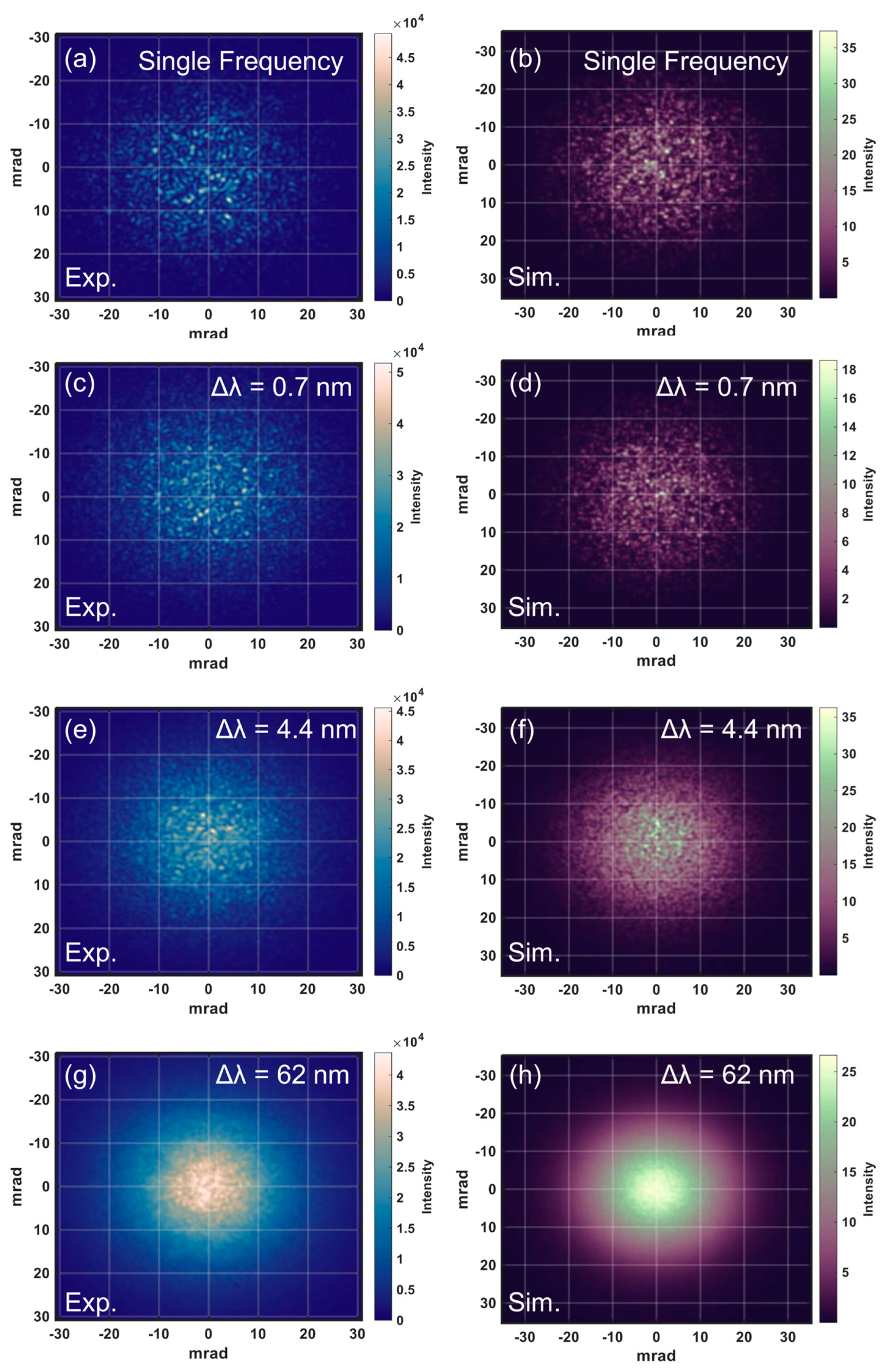
Experimental and simulated speckle patterns obtained using the four coherent illumination sources described in Section 2.1 are shown in Figure 3. For the single-frequency laser case, the spatial speckle was well-developed, exhibiting the classical bright and dark regions with no discernible pattern. As the laser linewidth increased, the area of a single speckle remained the same, but the image contrast was reduced; that is, the amplitude of each speckle was reduced with respect to the background. The spatial speckles are still visible even in the superluminescent diode pattern (Figure 3d), though the contrast is low. The simulated speckle patterns match the experimental patterns qualitatively, with a similar decrease in speckle contrast with increasing linewidth.
3.2. Regions of Interest and Speckle Contrast
Within the regions of interest chosen for the speckle contrast and reflectance calculations, both the spatial speckle and decreasing speckle contrast can be observed (Figure 4). The line scans shown in Figure 4f indicate the spatial speckle sizes remain unchanged throughout the experiment series at 8 to 10 pixels, while the relative amplitudes of the speckles decrease with increasing laser linewidth. The average speckle size (A) can be estimated based on the monochromatic wavelength and imaging f-number as [25]:
where F is the f-number of the imaging system, and λ is the wavelength of the illumination source. For the imaging system used here, f = 16 and λ = 1000 nm (on average), which results in a speckle area of 256 μm2. The speckle area in Figure 4 is approximately 310 μm2 using a speckle radius of 4.5 pixels.
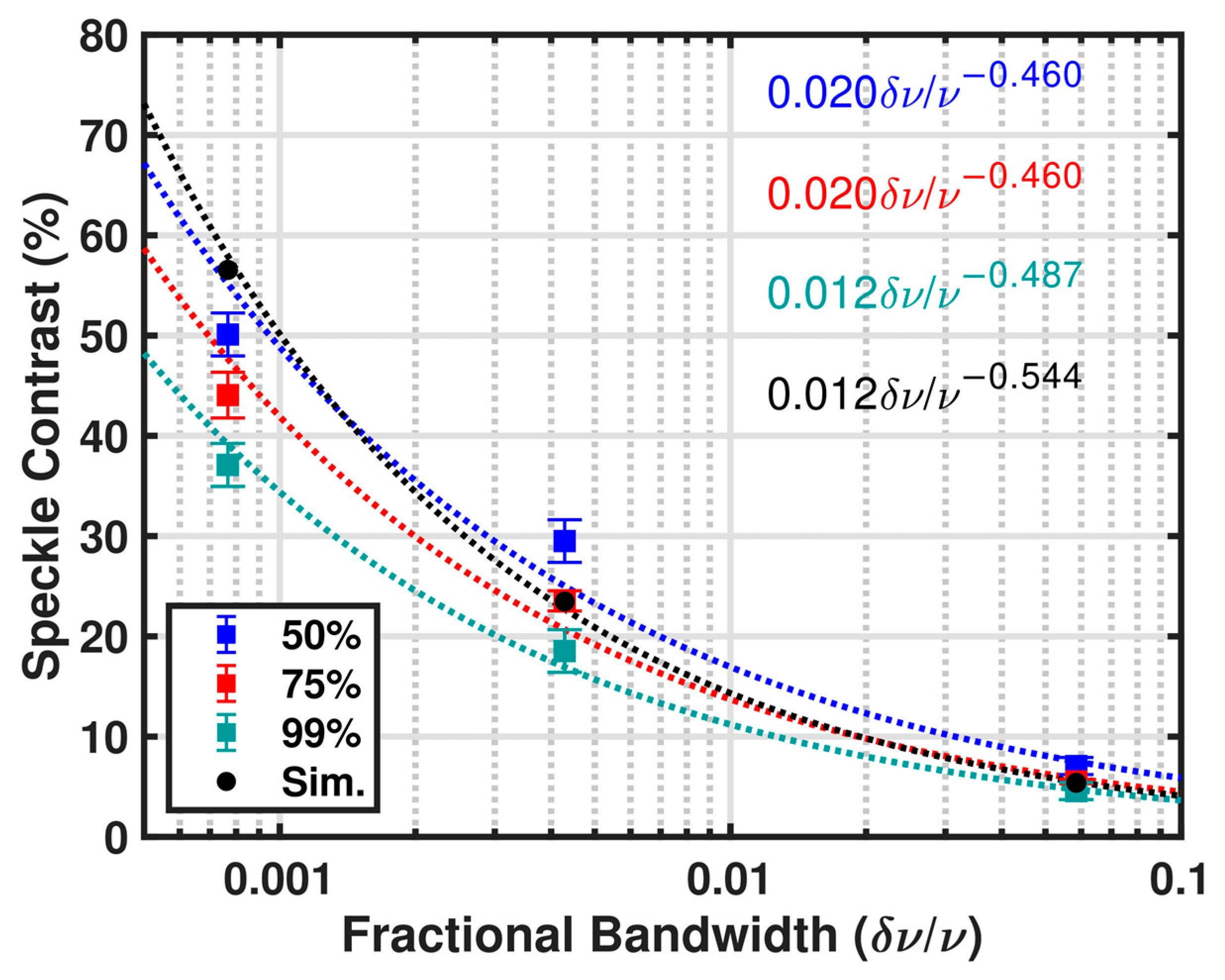
From each of the four speckle pattern ROIs for each imaging condition (illumination source and reflectance target), we calculated the speckle contrast as a ratio of the standard deviation to the mean value, including the speckle contrast mean and standard deviation for each imaging condition. From theory, a decrease in temporal coherence (described by the coherence length) reduces the speckle contrast (C) in the following manner [32]:
where δν is the frequency linewidth of the source, ν is the frequency of the illumination source, σ is the surface roughness of the screen, λ is the center wavelength of the source, θo is the observation angle, and θi is the incidence angle. Under constant imaging, the speckle contrast from Equation (5) will change with the normalized linewidth (δν/ν) as:
Figure 5 shows the results for the three illumination line widths used in the temporal speckle analysis (i.e., the 0.7 nm, 4.4 nm, and 62 nm linewidth sources). The speckle contrast for each of the three illumination sources was calculated as described above, with the white-light speckle noise (2.4 to 2.8%, depending on the target) subtracted from them. The simulated image speckle contrast was calculated in an identical way, using the central, equivalent 57 × 57-pixel region of each pattern. Speckle contrast for the single-frequency source was measured to be 60 to 65%, which means that the spatial speckle noise is a limited case for these illumination and imaging conditions.
Finally, we calculated the reflectance values using the mean value within the ROI for each target and illumination source and the method described in Section 2.2 to assess the effect of speckle noise reduction on reflectance precision. The results are shown in Figure 6a for all five illumination sources, with the reflectance precision for the three sources used in the speckle contrast study shown in Figure 6b. For the single-frequency source, a linewidth of 30 pm was assigned as this was the lower measurement limit of our optical spectrum analyzer, but these data were not used to calculate the power law fit in Figure 6b. For the white light source, there is no linewidth, but to compare it to the other sources, we assigned it a normalized linewidth of 1 for plotting purposes.
4. Discussion
Our speckle contrast reduction results (power low exponent of −0.46 to −0.49) are quantitatively similar to both with theory (exponent of −0.5) and with the simulated speckle pattern results (exponent of −0.54). Differences from theory likely stem from the irregular spectral shapes of the Dual Mode and Fabry–Perot sources, compared to the theory, which assumes a Gaussian spectral shape defined by the 1/e bandwidth. Similar results, as shown here, have been reported with respect to reducing speckle noise in laser projector sources. Yu and co-authors reported speckle contrast reduction slightly greater than predicted from theory using a step-chirped quasi-phase-matched device for second harmonic generation at 532 nm [32]. Kuksenkov and co-authors used multiple separated emission lines that led to a factor of ~1.7 in speckle reduction compared to the single-line case [33].
We found the reflectance measurement precision, as defined by the 3σ standard deviation of the relative reflectance of the four speckle patterns, increased significantly over the tested linewidth range. Table 2 lists the relative reflectance values and 3σ standard deviations for the entire experimental series for each of the three targets. Compared to the speckle contrast data, however, the variation of reflectance precision values was much higher. The power law fits for the speckle contrast data had r-squared values greater than 0.97, while the reflectance data r-squared values varied between 0.7 and 0.9. We hypothesize this difference is due to the small-number statistics at play in the reflectance measurements (population of 4), while the speckle contrast measurements were based on the standard deviation of all the speckle cells within each ROI (roughly 30 speckle cells per ROI). The average exponent for the speckle contrast power law fits was −0.48, while it was −0.43 for the reflectance measurements. From the three reflectance targets, the standard deviation of these exponents for both experiments was ~0.15. We hypothesize that the difference in power law fits between the speckle contrast and reflectance measurements has a statistical basis due to using only three reflectance standards and four speckle patterns per illumination source (n = 12) compared to the dozens of speckles included in each speckle contrast image.
The results here validate experimentally that at least 80% to 85% of the theoretical reduction in speckle contrast and a corresponding increase in reflectance precision is realizable by reducing the coherence of the laser illumination source, as measured by the normalized linewidth. This confirms that high-spatial-resolution laser reflectance spectroscopy is achievable beyond the spatial speckle limit by purposefully increasing the laser linewidth. Thus, bandwidth widening must be balanced with the laser source efficiency and required spectral bandwidth to resolve features of interest.
Modification of the spectral bandwidth of the laser source can be categorized using two major architectures: fiber and solid-state laser. Fiber lasers have been developed for the fundamental wavelength range from 0.6 to 3.4 µm [40]. These lasers typically achieve sufficient output energy for remote sensing applications through one or more stages of fiber amplification. To spectrally broaden these sources, a seed laser with a sufficient spectral width or structure can be utilized to achieve the desired performance. The wide variety of wavelength regions for fiber lasers makes them well-suited for the creation of the desired wavelength. For solid-state optical parametric oscillators (OPOs), linewidth broadening is inherently more difficult and is typically achieved through the introduction of shorter optical pulses and additional longitudinal modes [41]. When careful attention is paid to longitudinal mode formation in the cavity, mode beating can lead to not only larger spectral width but higher frequency conversion efficiency to other wavelengths as well. Pump divergence may also offer a method by which the linewidth can be purposefully widened [42].
For planetary reflectance spectroscopy, mineral and volatile reflectance bands are wide enough that flight-qualified passive spectrometers such as those on the Chandrayaan-1 mission [43], the Volatiles Investigating Polar Exploration Rover (VIPER) mission [44,45], and the Lunar Trailblazer mission [46,47] have spectral channels widths between 10 and 20 nm. Significant reflectance precision improvement, then, is available by broadening near- and mid-infrared laser sources from the nominal ~0.1 to 1 nm linewidth to ~10 nm. Based on our tests here, this should result in a precision increase in a factor of nearly 3.
5. Conclusions
We have experimentally verified the reduction in speckle contrast and subsequent increase in laser reflectance precision from linewidth broadening in the near-infrared in order to improve the design of laser reflectance spectrometers. We performed speckle imaging using calibrated reflectance targets and compared the experimental speckle patterns to both theoretical speckle contrast levels and theoretical speckle area, as well as to simulated speckle patterns derived from propagation using the Fast Fourier Transform. We observed a speckle contrast reduction very close to that predicted by theory (an exponent of −0.48 measured vs. −0.5 from theory). The experimental reflectance precision increase was at least 80%, which is expected from theory, which suggests laser linewidth broadening is a viable method of increasing reflectance precision without spatial averaging for lunar and planetary laser spectrometry. Based on the spectral sampling of current and upcoming lunar infrared spectrometers, linewidth broadening to the 10 nm level would be acceptable from a spectroscopic standpoint and would improve the speckle SNR by a factor of 3 or more.
Author Contributions
Conceptualization, D.R.C. and X.S.; methodology, D.R.C. and G.B.C.; software, D.R.C. and G.B.C.; formal analysis, D.R.C. and G.B.C.; investigation, all; resources, D.R.C. and X.S.; data curation, G.B.C.; writing—original draft preparation, D.R.C.; writing—review and editing, all.; visualization, D.R.C.; All authors have read and agreed to the published version of the manuscript.
Funding
This research is funded by the NASA Science Mission Directorate (SMD) Planetary Instrument Concepts for the Advancement of Solar System Observations (PICASSO) program under award 22-PICASSO22-0001 and the Development and Advancement of Lunar Instruments (DALI) program under award 22-DALI_2-0018.
Data Availability Statement
Raw data from the speckle experiments, along with experimenter notes and image metadata, are available at the following archive DOI:10.5281/zenodo.10999770.
Acknowledgments
We acknowledge assistance with pathfinder speckle experiments from Demetrios Poulios and a discussion with Paul Lucey on laser reflectance measurements.
Conflicts of Interest
The authors declare no conflicts of interest.
References
- Adams, J.B. Lunar and Martian Surfaces: Petrologic Significance of Absorption Bands in the Near-Infrared. Science 1968, 159, 1453–1455. [Google Scholar] [CrossRef] [PubMed]
- McCord, T.B. Color Differences on the Lunar Surface. J. Geophys. Res. 1969, 74, 3131–3142. [Google Scholar] [CrossRef]
- Nozette, S.; Rustan, P.; Pleasance, L.P.; Kordas, J.F.; Lewis, I.T.; Park, H.S.; Priest, R.E.; Horan, D.M.; Regeon, P.; Lichtenberg, C.L.; et al. The Clementine Mission to the Moon: Scientific Overview. Science 1994, 266, 1835–1839. [Google Scholar] [CrossRef] [PubMed]
- Smith, M.; Craig, D.; Herrmann, N.; Mahoney, E.; Krezel, J.; McIntyre, N.; Goodliff, K. The Artemis Program: An Overview of NASA’s Activities to Return Humans to the Moon. In Proceedings of the 2020 IEEE Aerospace Conference, Big Sky, MT, USA, 7–14 March 2020; IEEE: Piscataway, NJ, USA, 2020; pp. 1–10. [Google Scholar]
- Kleinhenz, J.E.; Paz, A. Case Studies for Lunar ISRU Systems Utilizing Polar Water. In Proceedings of the ASCEND 2020: American Institute of Aeronautics and Astronautics, Virtual, 16 November 2020. [Google Scholar]
- Fisher, E.A.; Lucey, P.G.; Lemelin, M.; Greenhagen, B.T.; Siegler, M.A.; Mazarico, E.; Aharonson, O.; Williams, J.-P.; Hayne, P.O.; Neumann, G.A.; et al. Evidence for Surface Water Ice in the Lunar Polar Regions Using Reflectance Measurements from the Lunar Orbiter Laser Altimeter and Temperature Measurements from the Diviner Lunar Radiometer Experiment. Icarus 2017, 292, 74–85. [Google Scholar] [CrossRef] [PubMed]
- Brown, H.M.; Boyd, A.K.; Denevi, B.W.; Henriksen, M.R.; Manheim, M.R.; Robinson, M.S.; Speyerer, E.J.; Wagner, R.V. Resource Potential of Lunar Permanently Shadowed Regions. Icarus 2022, 377, 114874. [Google Scholar] [CrossRef]
- Spudis, P.D. The Value of the Moon: How to Explore, Live, and Prosper in Space Using the Moon’s Resources; Smithsonian Books: Washington, DC, USA, 2016; ISBN 978-1-58834-503-5. [Google Scholar]
- Lucey, P.G.; Petro, N.; Hurley, D.M.; Farrell, W.M.; Prem, P.; Costello, E.S.; Cable, M.L.; Barker, M.K.; Benna, M.; Dyar, M.D.; et al. Volatile Interactions with the Lunar Surface. Geochemistry 2021, 82, 125858. [Google Scholar] [CrossRef]
- Potter, R.W.K.; Collins, G.S.; Kiefer, W.S.; McGovern, P.J.; Kring, D.A. Constraining the Size of the South Pole-Aitken Basin Impact. Icarus 2012, 220, 730–743. [Google Scholar] [CrossRef]
- Moriarty, D.P.; Pieters, C.M. The Character of South Pole-Aitken Basin: Patterns of Surface and Subsurface Composition. J. Geophys. Res. Planets 2018, 123, 729–747. [Google Scholar] [CrossRef]
- Speyerer, E.J.; Robinson, M.S. Persistently Illuminated Regions at the Lunar Poles: Ideal Sites for Future Exploration. Icarus 2013, 222, 122–136. [Google Scholar] [CrossRef]
- Bussey, D.B.J.; McGovern, J.A.; Spudis, P.D.; Neish, C.D.; Noda, H.; Ishihara, Y.; Sørensen, S.-A. Illumination Conditions of the South Pole of the Moon Derived Using Kaguya Topography. Icarus 2010, 208, 558–564. [Google Scholar] [CrossRef]
- Mazarico, E.; Barker, M.K.; Jagge, A.M.; Britton, A.W.; Lawrence, S.J.; Bleacher, J.E.; Petro, N.E. Sunlit Pathways between South Pole Sites of Interest for Lunar Exploration. Acta Astronaut. 2023, 204, 49–57. [Google Scholar] [CrossRef]
- Lucey, P.G.; Hayne, P.O.; Costello, E.; Green, R.; Hibbitts, C.; Goldberg, A.; Mazarico, E.; Li, S.; Honniball, C. The Spectral Radiance of Indirectly Illuminated Surfaces in Regions of Permanent Shadow on the Moon. Acta Astronaut. 2021, 180, 25–34. [Google Scholar] [CrossRef]
- Cloutis, E.A.; Caudill, C.; Lalla, E.A.; Newman, J.; Daly, M.; Lymer, E.; Freemantle, J.; Kruzelecky, R.; Applin, D.; Chen, H.; et al. LunaR: Overview of a Versatile Raman Spectrometer for Lunar Exploration. Front. Astron. Space Sci. 2022, 9, 1016359. [Google Scholar] [CrossRef]
- Wang, A.; Jolliff, B.L.; Haskin, L.A. Raman Spectroscopy as a Method for Mineral Identification on Lunar Robotic Exploration Missions. J. Geophys. Res. 1995, 100, 21189–21199. [Google Scholar] [CrossRef]
- Lucey, P.; Petro, N.; Hurley, D.; Farrell, W.; Sun, X.; Green, R.; Greenberger, R.; Cameron, D. The Lunar Volatiles Orbiter: A Lunar Discovery Mission Concept. In Proceedings of the 2017 Annual Meeting of the Lunar Exploration Analysis Group, Columbia, MD, USA, 9–11 October 2017; Volume 2041, p. 5048. [Google Scholar]
- Cohen, B.A.; Hayne, P.O.; Greenhagen, B.; Paige, D.A.; Seybold, C.; Baker, J. Lunar Flashlight: Illuminating the Lunar South Pole. IEEE Aerosp. Electron. Syst. Mag. 2020, 35, 46–52. [Google Scholar] [CrossRef]
- Cohen, B.A.; Petersburg, R.R.; Cremons, D.R.; Russell, P.S.; Hayne, P.O.; Greenhagen, B.T.; Paige, D.A.; Camacho, J.M.; Cheek, N.; Sullivan, M.T.; et al. Lunar Flashlight Science Ground and Flight Measurements and Operations Using a Multi-Band Laser Reflectometer. Icarus 2024, 413, 116013. [Google Scholar] [CrossRef]
- Lucey, P.G.; Neumann, G.A.; Riner, M.A.; Mazarico, E.; Smith, D.E.; Zuber, M.T.; Paige, D.A.; Bussey, D.B.; Cahill, J.T.; McGovern, A.; et al. The Global Albedo of the Moon at 1064 Nm from LOLA. J. Geophys. Res. Planets 2014, 119, 1665–1679. [Google Scholar] [CrossRef]
- Hayne, P.O.; Hendrix, A.; Sefton-Nash, E.; Siegler, M.A.; Lucey, P.G.; Retherford, K.D.; Williams, J.-P.; Greenhagen, B.T.; Paige, D.A. Evidence for Exposed Water Ice in the Moon’s South Polar Regions from Lunar Reconnaissance Orbiter Ultraviolet Albedo and Temperature Measurements. Icarus 2015, 255, 58–69. [Google Scholar] [CrossRef]
- Lemelin, M.; Lucey, P.G.; Neumann, G.A.; Mazarico, E.M.; Barker, M.K.; Kakazu, A.; Trang, D.; Smith, D.E.; Zuber, M.T. Improved Calibration of Reflectance Data from the LRO Lunar Orbiter Laser Altimeter (LOLA) and Implications for Space Weathering. Icarus 2016, 273, 315–328. [Google Scholar] [CrossRef]
- Cremons, D.R.; Honniball, C.I. Simulated Lunar Surface Hydration Measurements Using Multispectral Lidar at 3 Μm. Earth Space Sci. 2022, 9, e2022EA002277. [Google Scholar] [CrossRef] [PubMed]
- Goodman, J.W. Speckle Phenomena in Optics: Theory and Applications, 2nd ed.; The International Society for Optical Engineering: Bellingham, WA, USA, 2020; ISBN 978-1-5106-3149-6. [Google Scholar]
- Cassé, V.; Gibert, F.; Edouart, D.; Chomette, O.; Crevoisier, C. Optical Energy Variability Induced by Speckle: The Cases of MERLIN and CHARM-F IPDA Lidar. Atmosphere 2019, 10, 540. [Google Scholar] [CrossRef]
- Akram, M.N.; Chen, X. Speckle Reduction Methods in Laser-Based Picture Projectors. Opt. Rev. 2016, 23, 108–120. [Google Scholar] [CrossRef]
- Lee, S.; Kim, D.; Nam, S.-W.; Lee, B.; Cho, J.; Lee, B. Light Source Optimization for Partially Coherent Holographic Displays with Consideration of Speckle Contrast, Resolution, and Depth of Field. Sci. Rep. 2020, 10, 18832. [Google Scholar] [CrossRef] [PubMed]
- Tran, T.-T.-K.; Svensen, Ø.; Chen, X.; Akram, M.N. Speckle Reduction in Laser Projection Displays through Angle and Wavelength Diversity. Appl. Opt. 2016, 55, 1267–1274. [Google Scholar] [CrossRef] [PubMed]
- Kozacki, T.; Chlipala, M. Color Holographic Display with White Light LED Source and Single Phase Only SLM. Opt. Express 2016, 24, 2189–2199. [Google Scholar] [CrossRef]
- Trisnadi, J.I. Speckle Contrast Reduction in Laser Projection Displays; Wu, M.H., Ed.; SPIE Press: San Jose, CA, USA, 2002; pp. 131–137. [Google Scholar]
- Yu, N.E.; Choi, J.W.; Kang, H.; Ko, D.-K.; Fu, S.-H.; Liou, J.-W.; Kung, A.H.; Choi, H.J.; Kim, B.J.; Cha, M.; et al. Speckle Noise Reduction on a Laser Projection Display via a Broadband Green Light Source. Opt. Express 2014, 22, 3547–3556. [Google Scholar] [CrossRef] [PubMed]
- Kuksenkov, D.V.; Roussev, R.V.; Li, S.; Wood, W.A.; Lynn, C.M. Multiple-Wavelength Synthetic Green Laser Source for Speckle Reduction; Vodopyanov, K.L., Ed.; SPIE Press: San Francisco, CA, USA, 2011; p. 79170B. [Google Scholar]
- Ehret, G.; Bousquet, P.; Pierangelo, C.; Alpers, M.; Millet, B.; Abshire, J.B.; Bovensmann, H.; Burrows, J.P.; Chevallier, F.; Ciais, P.; et al. MERLIN: A French-German Space Lidar Mission Dedicated to Atmospheric Methane. Remote Sens. 2017, 9, 1052. [Google Scholar] [CrossRef]
- Riris, H.; Li, S.; Numata, K.; Wu, S.; Yu, A.; Burris, J.; Krainak, M.; Abshire, J. LIDAR Technology for Measuring Trace Gases on Mars and Earth. In Proceedings of the Lidar Remote Sensing for Environmental Monitoring XII, San Diego, CA, USA, 21–22 August 2011; p. 8159. [Google Scholar]
- Abshire, J.B.; Riris, H.; Allan, G.R.; Weaver, C.J.; Mao, J.; Sun, X.; Hasselbrack, W.E.; Kawa, S.R.; Biraud, S. Pulsed Airborne Lidar Measurements of Atmospheric CO2 Column Absorption. Tellus B Chem. Phys. Meteorol. 2010, 62, 770. [Google Scholar] [CrossRef]
- Pierrottet, D.F.; Amzajerdian, F.; Petway, L.B.; Hines, G.D.; Barnes, B. Field Demonstration of a Precision Navigation Lidar System for Space Vehicles. In Proceedings of the AIAA Guidance, Navigation, and Control (GNC) Conference: American Institute of Aeronautics and Astronautics, Boston, MA, USA, 19 August 2013. [Google Scholar]
- Dunmeyer, D. Laser Speckle Modeling for Three-Dimensional Metrology and LADAR. Master’s Thesis, Massachusetts Institute of Technology, Cambridge, MA, USA, 2001. [Google Scholar]
- Schwenger, F.; Braesicke, K. Simulation of Laser Speckle Patterns Generated by Random Rough Surfaces. In Proceedings of the Infrared Imaging Systems: Design, Analysis, Modeling, and Testing XXXI, Online, 23 April 2020; Holst, G.C., Haefner, D.P., Eds.; SPIE Press: San Jose, CA, USA; p. 14. [Google Scholar]
- Paschotta, R. Field Guide to Laser Pulse Generation; SPIE Field Guides; SPIE Press: Bellingham, WA, USA, 2008; ISBN 978-0-8194-7248-9. [Google Scholar]
- Siegman, A.E. Lasers; University Science Books: Mill Valley, CA, USA, 1986; ISBN 978-0-935702-11-8. [Google Scholar]
- Brosnan, S.; Byer, R. Optical Parametric Oscillator Threshold and Linewidth Studies. IEEE J. Quantum Electron. 1979, 15, 415–431. [Google Scholar] [CrossRef]
- Green, R.; Pieters, C.; Mouroulis, P.; Eastwood, M.; Boardman, J.; Glavich, T.; Isaacson, P.; Annadurai, M.; Besse, S.; Barr, D.; et al. The Moon Mineralogy Mapper (M3) Imaging Spectrometer for Lunar Science: Instrument Description, Calibration, on-Orbit Measurements, Science Data Calibration and on-Orbit Validation. J. Geophys. Res. Planets 2011, 116, E00G19. [Google Scholar] [CrossRef]
- Colaprete, A.; Andrews, D.; Bluethmann, W.; Elphic, R.C.; Bussey, B.; Trimble, J.; Zacny, K.; Captain, J.E.; Colaprete, A.; Andrews, D.; et al. An Overview of the Volatiles Investigating Polar Exploration Rover (VIPER) Mission. In Proceedings of the American Geophysical Union, San Francisco, CA, USA, 9–13 December 2019; Volume 2019, p. P34B–03. [Google Scholar]
- Roush, T.; Colaprete, A.; Cook, A.; Bielawski, R.; Ennico-Smith, K.; Noe Dobrea, E.; Benton, J.; Forgione, J.; White, B.; McMurray, R.; et al. The Volatiles Investigating Polar Exploration Rover (VIPER) Near Infrared Volatile Spectrometer System (NIRVSS). In Proceedings of the Lunar and Planetary Science Conference, Online, 15–19 March 2021; p. 1678. [Google Scholar]
- Bender, H.A.; Smith, C.D.; Ehlmann, B.L.; Thompson, D.R.; Vinckier, Q.P.; Mouroulis, P. Optical Design and Performance of the Lunar Trailblazer High-Resolution Volatiles and Minerals Moon Mapper (HVM3). In Proceedings of the Imaging Spectrometry XXV: Applications, Sensors, and Processing, San Diego, CA, USA, 22 August 2022; Ientilucci, E.J., Bradley, C.L., Eds.; SPIE Press: San Diego, CA, USA, 2022; p. 3. [Google Scholar]
- Ehlmann, B.L.; Klima, R.L.; Seybold, C.C.; Klesh, A.T.; Au, M.H.; Bender, H.A.; Bennett, C.L.; Blaney, D.L.; Bowles, N.; Calcutt, S.; et al. NASA’s Lunar Trailblazer Mission: A Pioneering Small Satellite for Lunar Water and Lunar Geology. In Proceedings of the 2022 IEEE Aerospace Conference (AERO), Big Sky, MT, USA, 5–12 March 2022; IEEE: Piscataway, NJ, USA, 2022; pp. 1–14. [Google Scholar]
Figure 1.
Spectra of the three illumination sources used for the direct speckle comparison. (a) Dual mode pump diode, (b) Fabry–Perot diode, and (c) superluminescent diode.
Figure 1.
Spectra of the three illumination sources used for the direct speckle comparison. (a) Dual mode pump diode, (b) Fabry–Perot diode, and (c) superluminescent diode.

Figure 2.
(a) Speckle imaging experimental setup including fiber-optic reflective collimator (RC), Spectralon targets (ST), 25 mm FL imaging lens (IL), and CMOS camera (Cam). (b) CMOS camera image of the 99% reflective target illuminated with the white-light source in the geometry from (a). Dark spots on the Spectralon target were due to lens imperfections, and these image regions were excluded from all quantitative analyses.

Figure 3.
Representative speckle patterns from the experiment series and their corresponding simulated speckle patterns. All experimental images shown here were obtained using the 99% reflective target. Each row shows an experimental speckle pattern and its corresponding simulated speckle patterns. (a,b) Single-frequency diode, (c,d) Dual-mode pump diode, (e,f) Fabry–Perot diode, (g,h) Superluminescent diode. The laser linewidth or identifiers are given in the upper left-hand corner of each frame. Each frame was cropped from the full image to be 350 × 350 pixels, centered on the centroid of the laser spot.

Figure 4.
Speckle pattern development as a function of increasing laser linewidth for the regions of interest is used for speckle contrast and reflectance calculations. All images shown here were obtained using the 99% reflective target. (a) Single-frequency diode, (b) Dual-mode pump diode, (c) Fabry–Perot diode, (d) Superluminescent diode, (e) white light. The laser linewidth or identifiers are given in the upper left-hand corner of each frame. The color scale denotes image intensity, and the full scale is based on the entire background-subtracted image, not the ROI. (f) Horizontal line scans for each source taken from the center 10 pixels ROI. The y-axis represents relative intensity defined by the pixel intensity values divided by the average over the whole linescan.

Figure 5.
Speckle contrast results from temporal coherence study. The blue dots represent data from the 50% reflectance targets, red dots from the 75% reflectance targets, and green from the 99% reflectance targets. The error bars denote one standard deviation from the population of four speckle pattern measurements. The dotted lines denote best-fit power law curves for each target, with the fit equations given in the inset.

Figure 6.
(a) Reflectance measurements as a function of normalized linewidth for the five illumination sources in this study. The blue dots represent data from the 50% reflectance targets, red dots from the 75% reflectance targets, and green from the 99% reflectance targets. The error bars here denote 3σ standard deviation from the four speckle pattern measurements. (b) Reflectance precision (3σ) for the 0.7 nm, 4.4 nm, and 62 nm linewidth laser sources. The dotted lines denote best-fit power law curves for each target, with the fit equations given in the inset.


Table 1.
Parameters for the five light sources used for the speckle experiments. Each diode laser was a 14-pin butterfly package. The white light source was free-space coupled to illuminate the target.
Table 1.
Parameters for the five light sources used for the speckle experiments. Each diode laser was a 14-pin butterfly package. The white light source was free-space coupled to illuminate the target.
| Illumination Source | Center Wavelength | Linewidth 1 | Normalized Linewidth 2 |
|---|---|---|---|
| Single Frequency Diode | 1063.9894 nm | <0.03 nm | 2.6 × 10⁻⁵ |
| Dual Mode Pump Diode | 975.69 nm | 0.75 nm | 7.7 × 10⁻⁴ |
| Fabry–Perot Diode | 1034.4 nm | 4.4 nm | 0.0043 |
| Superluminescent Diode | 1068 nm | 62.5 nm | 0.059 |
| Halogen White Light Source | 360–2400 nm 3 | ||
1 Bandwidths for the laser sources were all calculated using the second moment of the laser spectrum. 2 Normalized linewidth is defined here as the linewidth divided by the center wavelength. 3 The white light source is described here by its specified spectral range.
Table 2.
Mean reflectance values and 3σ precision values for the entire experiment series.
| Laser Source | Normalized Linewidth | 50% Target | 75% Target | 99% Target 1 |
|---|---|---|---|---|
| Single Frequency Diode | 2.6 × 10⁻⁵ | 0.6 ± 0.3 | 0.8 ± 0.6 | 0.99 ± 0.9 |
| Dual Mode Pump Diode | 7.7 × 10⁻⁴ | 0.5 ± 0.4 | 0.9 ± 0.3 | 0.99 ± 0.3 |
| Fabry–Perot Diode | 0.0043 | 0.5 ± 0.1 | 0.8 ± 0.3 | 0.99 ± 0.3 |
| Superluminescent Diode | 0.059 | 0.56 ± 0.06 | 0.83 ± 0.05 | 0.99 ± 0.05 |
| Halogen White Light Source | N/A | 0.47 ± 0.01 | 0.74 ± 0.01 | 0.99 ± 0.03 |
1 The reflectance values for each source were normalized by the average intensity using the 99% target, which fixes the mean reflectance at 0.99 for those experiments.
Disclaimer/Publisher’s Note: The statements, opinions and data contained in all publications are solely those of the individual author(s) and contributor(s) and not of MDPI and/or the editor(s). MDPI and/or the editor(s) disclaim responsibility for any injury to people or property resulting from any ideas, methods, instructions or products referred to in the content. |
© 2024 by the authors. Licensee MDPI, Basel, Switzerland. This article is an open access article distributed under the terms and conditions of the Creative Commons Attribution (CC BY) license (https://creativecommons.org/licenses/by/4.0/).
Share and Cite
MDPI and ACS Style
Cremons, D.R.; Clarke, G.B.; Sun, X. Speckle Noise Reduction via Linewidth Broadening for Planetary Laser Reflectance Spectrometers. Remote Sens. 2024, 16, 1515. https://0-doi-org.brum.beds.ac.uk/10.3390/rs16091515
AMA Style
Cremons DR, Clarke GB, Sun X. Speckle Noise Reduction via Linewidth Broadening for Planetary Laser Reflectance Spectrometers. Remote Sensing. 2024; 16(9):1515. https://0-doi-org.brum.beds.ac.uk/10.3390/rs16091515
Chicago/Turabian StyleCremons, Daniel R., Gregory B. Clarke, and Xiaoli Sun. 2024. "Speckle Noise Reduction via Linewidth Broadening for Planetary Laser Reflectance Spectrometers" Remote Sensing 16, no. 9: 1515. https://0-doi-org.brum.beds.ac.uk/10.3390/rs16091515
Note that from the first issue of 2016, this journal uses article numbers instead of page numbers. See further details here.