Correction Control Model of L-Index Based on VSC-OPF and BLS Method

Abstract

With the advancement of artificial intelligence (AI) technology, the real-time measurement and control technology of power systems has also progressed. This paper proposes a correction control model for L-indexes based on voltage stability constrained optimal power flow (VSC-OPF) and a broad learning system (BLS) (BLS-VSC-OPF). This model aims to quickly assess the system’s voltage stability and accurately correct the operation mode when the voltage stability indexes are out of the security range. Firstly, the BLS is used to predict the L-index and to analyze the voltage stability of the power system. Secondly, the approximate first-order sensitivity of the L-index is calculated by the combination of the BLS and the perturbation method. This method solves the problem of the complex sensitivity derivation process in the modeling process of the VSC-OPF model. Meanwhile, when the L-index exceeds the threshold, the BLS and VSC-OPF models are combined to correct this operation mode. The feasibility of the proposed method is verified by the simulation of IEEE-30, IEEE-118, and 1047 bus systems. Finally, the BLS-VSC-OPF model is compared with the linear programming correction model based on BLS (BLS-LPC). The results show that the BLS-VSC-OPF model provides a better correction and control performance.

1. Introduction

With the advancement of science and technology, the demand for new energy in the world is constantly expanding, which makes sustainable development an important issue [1]. Voltage stability control is inextricably linked to sustainability. Accurate voltage stability control can improve energy efficiency, thereby reducing the environmental pollution caused by energy exploitation and power generation, and promoting sustainable development of the environment. In recent years, the frequent occurrence of voltage collapse has led to many large-scale power outages, which has brought about a serious impact on the sustainable development of society and the economy [2]. Voltage stability control can not only reduce power loss and protect critical power equipment, but also ensure the stable operation of power systems, thus significantly improving their economic efficiency. In addition, voltage stability control can also effectively enhance the security and reliability of power systems, which provides an important guarantee for the long-term sustainable development of the power industry. In order to solve the problem of sustainable development, the combination of renewable energy and power grids has become a trend. However, the intermittency and uncertainty of renewable energy sources increase the complexity of voltage stability control [3]. It can be seen that voltage stability control is an important part of the sustainable development of power systems, which is closely related to sustainability. The problem of voltage stability has been widely studied and related research has been derived in many fields, including voltage stability assessment techniques in smart grids, voltage stability control techniques in renewable energy systems, voltage correction techniques in power system dynamics and control topics, etc. To achieve the sustainable development of power systems, finding a way to quickly evaluate and rectify the static voltage stability of a system has immense significance.

The existing problems mainly include how to quickly obtain the system’s voltage stability and correct the unstable operating state. The L-index is one of the effective means to measure a system’s voltage level. However, with the continuous expansion of the system, the calculation of the L-index becomes more complex, and the correction of an unstable operating state becomes more difficult. VSC-OPF can improve the voltage stability of a system effectively, but it is difficult to obtain the sensitivity of the L-index in the VSC-OPF model with the L-index as a constraint, because the calculation formula of the L-index involves the operation of absolute value. This paper introduces a BLS-VSC-OPF model, which is intended to enhance the voltage stability of power systems. The proposed model is designed to rapidly adapt to changes in the system’s operational conditions and predict the L-index of the system. Whenever the L-index exceeds the defined range, it can be promptly corrected. This method can obtain the L-index sensitivity of different operating modes through a simple perturbation process, which greatly simplifies the sensitivity computation and realizes the real-time measurement and correction control of system voltage stability. The main contributions of this paper can be summarized as follows:

The L-index prediction and analysis of the system are done by combining the broad learning system with the L-index calculation. To obtain the training and testing sets, the continuous power flow (CPF) method is utilized, followed by the training and testing of the BLS. Upon achieving the desired level of accuracy, the BLS is employed to predict the system’s L-index in real time.

A BLS is introduced into VSC-OPF for the first time. This technique is used to calculate the sensitivity of the L-index to the control variables in the system. With this, the complex derivation of the sensitivity equation in the traditional VSC-OPF method is avoided, and the amount of computation is reduced. In addition, this method does not require any load shedding measure. It can enhance the system voltage stability by adjusting the generator output, thus improving the economy of correction.

The proposed model is simulated and verified in IEEE-30, IEEE-118, and 1047 bus systems. The results of the simulation indicate that the model is capable of correcting the L-index and improving the voltage stability of the system in cases where the L-index exceeds the threshold value. In addition, to better demonstrate the superior performance of the proposed model, we conduct a comparative analysis between the BLS-LPC method and the proposed BLS-VSC-OPF method.

The rest of this paper is structured as follows: Section 2 describes the static voltage stability L-index in detail. Section 3 describes the traditional VSC-OPF method. Section 4 introduces the structure of the BLS and the modeling process of the BLS-VSC-OPF model. Section 5 shows the simulation analysis of the proposed model and compares it with other correction models. Finally, the conclusion is given in Section 6.

2. Literature Review

Several static voltage stability indices have been proposed to accurately determine the voltage stability of a system. For instance, Musirin proposed a fast voltage stability index (FVSI), Moghavemmi suggested several stability indexes (Lmn, Lp, VCPI), and Milosevic proposed the voltage stability load bus index (VSLBI) [4,5,6,7,8]. Kessel introduced an L-index of local voltage stability, which can quickly evaluate the voltage stability of a system by solving power flow (PF) [9]. P-A Lof et al. [10] proposed an evaluation method based on the minimum singular value of the Jacobian matrix. If the minimum singular value is zero, the voltage is close to collapse. Althowibi and Mustafa proposed a method and index based on network sensitivity to determine the voltage stability and stability margin [11]. Houhe Chen and Tao Jiang proposed an evaluation method based on voltage sensitivity, which is based on the existing L-index [12]. Currently, the L-index is widely used in the voltage stability evaluation of power systems because of its simple structure and accurate evaluation ability.

When the voltage stability index of a system exceeds the safe range, it becomes imperative to take corrective measures promptly to prevent voltage collapse accidents. Reference [13] proposed a nonlinear programming methodology to correct voltage instability by centralized load shedding (LS) based on the dynamic security assessment (DSA) computations when disturbances threatening the system are detected. Reference [14] utilized the direct equilibrium tracing method to determine the saddle node bifurcation point such that the minimum control actions were derived, and finally, voltage correction was performed by shedding loads. Furthermore, a load shedding algorithm is proposed in [15], which applies a higher percentage of load shedding to buses with relatively weak voltage stability, thus obtaining satisfactory voltage stability while improving the frequency response of the grid. However, it is imperative to exercise caution when implementing load shedding, as it carries the risk of partial power outages. Recently, some research has taken reactive power compensation devices as an entry point to finding the optimal location and size of reactive power compensation devices, with the aim of enhancing voltage stability and reliability [16,17].

Although the aforementioned approaches can address voltage instability, they fail to achieve an optimal solution. To make power systems more economical and stable, scholars have proposed the VSC-OPF model by combining voltage stability with the OPF, which has made some progress. In [18], the L-index was added to the traditional OPF model as a constraint. The primal-dual interior point method was used to solve the model, which improves the voltage stability of the system. In [19], the voltage collapse proximity index (VCPI) was used as a constraint for the voltage stability. This method can not only improve voltage stability but also reduce power loss. Reference [20] proposed an improved multi-objective OPF model considering the voltage security margin. This model optimizes the comprehensive operating costs of the system while ensuring that the system operates at the desired load margin. Despite the above progress, the inclusion of voltage stability constraints still makes the problem of OPF more complicated. Therefore, the relaxed convex VSC-OPF models are proposed. In [21], the voltage stability condition of VSC-OPF was reformulated as a set of second-order conic constraints in the transformed variable space. This method can effectively suppress the stability stress of the system, and its sparse approximation has a noticeable acceleration effect in large systems. In addition, considering the problem of solution cost and precision in voltage stability assessment, reference [22] establishes the formulation and convexification of VSC-OPF. This model considers PV-PQ bus type switching, which co-optimizes the generation dispatch and bus type profile.

Following a thorough review of previous studies, it has become apparent that conventional voltage stability correction methods and VSC-OPF studies are challenged by complex derivation and modeling processes, which consume a great deal of time and memory in their calculations. Furthermore, such methods do not facilitate quick determination of the voltage stability of the system through operating parameters. Fortunately, various neural networks and intelligent algorithms have emerged with rapid advances in AI technology. Many scholars have introduced AI into power systems, providing a new way to solve the problems mentioned above. Reference [23] proposed a DNN-based distributed voltage stability online monitoring method for large-scale power grids, using DNN to predict the load impedance modulus margin (LIMM) of weak nodes so the system operator can judge the current operation state of the system and make the corresponding measures in time. Meanwhile, reference [24] suggests a deep reinforcement learning (DRL) framework based on a graph convolutional network (GCN) to address voltage stabilization control problems caused by topology changes in power systems. Since DRL methods are usually assumed to learn through trial-and-error, which requires significant interactions, a novel deep feedback learning machine (DFLM) is designed in [25] to precisely predict future voltage violations after UVLS execution. There is also research showing that the BP neural network can evaluate the voltage stability state of a system with high precision and rapidly assist in a non-dominated sorting genetic algorithm improving the static voltage stability margin [26]. AI has also made progress in conjunction with OPF, such as speeding up the solution process [27] and reducing operating costs [28]. Reference [29] used a multi-objective particle swarm optimization to solve the single- and multi-objective OPF issues. Reference [30] combined the cuckoo search (CSA) method with sunflower optimization (SFO) to improve the performance of OPF solutions. Reference [31] proposed an energy management system (EMS) for the optimal operation of smart grids and microgrids by combining a fully connected neuronal network (FCN) with OPF. Furthermore, a parametric graph neural network (GNN) model was used in reference [32] to mimic the interior point solver to obtain the optimal solution, which can be applied to irregular large power systems. In [33], a sensitivity-informed DNN method is proposed to match the OPF optimizers and the partial derivatives with respect to the OPF parameter, which provides new ideas for solving the OPF problem. The emergence of BLS provides more possibilities for the combination of AI and power systems. To quickly assess the voltage stability and correct the voltage instability state of power systems, reference [34] established the prediction and linear correction model of the L-index based on BLS. Similarly, reference [35] used the BLS to conduct the CCT prediction analysis and correction control of power systems. Reference [36] proposed a state evaluation method of power systems based on BLS which improved the ability of power systems to quickly respond to emergencies. A mass of cases exists that demonstrates the effective use of AI technology to improve power systems. As such, the development of power systems that incorporate AI technology is a viable option.

3. Static Voltage Stability Index

The assessment of voltage stability is a critical aspect of power systems. In this regard, we propose the utilization of the L-index as a voltage stability index. This index is preferred over others due to its remarkable accuracy and low computational complexity. The L-index provides well-defined upper and lower limits. When 0 < L < 1, the system voltage is in a stable state; when L = 1, it is in a critical state; when L > 1, the voltage collapses [9]. To compute the L-index, the system nodes are first categorized into three sets: set G, which contains the generator and PV nodes of the system; set L, which includes all load nodes; and set K, which contains all contact nodes. The procedure for calculating the L-index is described below.

$$\left[\begin{array}{l}{I}_G\\ I_L\\ 0\end{array}\right]=\left[\begin{array}{ccc}{Y_{GG}}^{\prime }& {Y_{GL}}^{\prime }& {Y_{GK}}^{\prime }\\ {Y_{LG}}^{\prime }& {Y_{LL}}^{\prime }& {Y_{LK}}^{\prime }\\ {Y_{KG}}^{\prime }& {Y_{KL}}^{\prime }& {Y_{KK}}^{\prime }\end{array}\right]\left[\begin{array}{c}{V}_G\\ V_L\\ V_K\end{array}\right]$$

(1)

where, I_G and I_L represent the currents at the generator and load nodes, V_G and V_L represent the voltages at the generator and load nodes, V_K represents the voltage at the contact nodes, and Y_GG, Y_GL, Y_GK, Y_LG, Y_LL, Y_LK, Y_KG, Y_KL, and Y_KK are derived matrices of the node admittance matrix.

After eliminating the contact nodes, the above equation can be transformed into:

$$\left[\begin{array}{l}{I}_G\\ I_L\end{array}\right]=\left[\begin{array}{cc}{Y}_{GG}& Y_{GL}\\ Y_{LG}& Y_{LL}\end{array}\right]\left[\begin{array}{l}{V}_G\\ V_L\end{array}\right]$$

(2)

where $Y_{GG}={Y_{GG}}^{\prime }-{Y_{GK}}^{\prime }{{Y_{KK}}^{\prime }}^{-1}{Y_{KG}}^{\prime }$, $Y_{GL}={Y_{GL}}^{\prime }-{Y_{GK}}^{\prime }{{Y_{KK}}^{\prime }}^{-1}{Y_{KL}}^{\prime }$, and $Y_{LG}={Y_{LG}}^{\prime }-{Y_{LK}}^{\prime }{{Y_{KK}}^{\prime }}^{-1}{Y_{KG}}^{\prime }$, $Y_{LL}={Y_{LL}}^{\prime }-{Y_{LK}}^{\prime }{{Y_{KK}}^{\prime }}^{-1}{Y_{KL}}^{\prime }$. The above equation is rewritten as:

$$\left[\begin{array}{l}{I}_G\\ V_L\end{array}\right]=\left[\begin{array}{cc}{Y}_{GG}-Y_{GL}{Z}_{LL}{Y}_{LG}& Y_{GL}{Z}_{LL}\\ -Z_{LL}{Y}_{LG}& Z_{LL}\end{array}\right]\left[\begin{array}{l}{V}_G\\ I_L\end{array}\right]$$

(3)

where Z_LL = Y_LL⁻¹. Defining the load participation factor matrix F_LG = −Z_LLY_LG, the final expression of the L-index can be obtained as:

$$L_j=\left|1-{\displaystyle \sum _{k\in G}{F}_{jk}\frac{V_k}{V_j}\angle ({\theta }_{jk}+{\delta }_k-{\delta }_j)}\right|$$

(4)

where L_j is the L-index of load node j, F_jk and ${\theta }_{jk}$ are the amplitude and phase of the corresponding element in F_LG, V_k and ${\theta }_k$ are the voltage amplitude and phase of generator node k, and V_j and ${\theta }_j$ are the voltage amplitude and phase of load node j.

In the context of power systems, each load node is typically assigned an L-index that indicates the voltage status. Of particular importance is the highest L-index value, which is referred to as the L-index of the system and is a critical factor in evaluating system stability. It is important to control the L-index in order to ensure that the power system operates in a stable state and maintains a sufficient voltage stability margin.

4. Classic VSC-OPF Model

4.1. Objective Function

In the basic OPF model, the lowest operating cost of the system, as the objective function, can be written as the following expression:

$$\min f(x)={\displaystyle \sum _{i\in S_G}{P}_{Gi}}$$

(5)

where S_G is the set of system generator nodes and P_Gi is the active power of the generator.

4.2. Equality Constraints

Using the power equation as an equation constraint:

$$\{\begin{array}{c}{P}_{Gi}-P_{Di}-V_i{\displaystyle \sum _{j\in S_N}{V}_j{Y}_{ij}\cos {\theta }_{ij}=0}\\ Q_{Gi}-Q_{Di}-V_i{\displaystyle \sum _{j\in S_N}{V}_j{Y}_{ij}\sin {\theta }_{ij}=0}\end{array}\begin{array}{cc},& i\in S_N\end{array}$$

(6)

where S_N is the set of all nodes of the system, Q_Gi is the reactive power of the generator, P_Di and Q_Di are the active power and reactive power of the load, V_i and V_j are the voltage amplitudes of nodes i and j, Y_ij and ${\alpha }_{\mathrm{ij}}$ are the amplitude and phase of the transfer impedance between nodes i and j, and ${\theta }_{ij}={\delta }_i-{\delta }_j-{\alpha }_{ij}$, ${\delta }_{\mathrm{i}}$, and ${\delta }_j$ are the voltage phases of nodes i and j.

4.3. Inequality Constraints

To achieve an optimal solution for a system, it is necessary to restrict the active power of the generators, the reactive power of the reactive power supplies, and the voltage amplitude of the system nodes within a specific range. Inequality constraints are utilized to express these limitations in the traditional OPF model:

$$\{\begin{array}{c}{P}_{Gi}^{\min }\le P_{Gi}\le P_{Gi}^{\max }\begin{array}{cc},& i\in S_G\end{array}\\ Q_{Ri}^{\min }\le Q_{Ri}\le Q_{Ri}^{\max }\begin{array}{cc},& i\in S_R\end{array}\\ V_i^{\min }\le V_i\le V_i^{\max }\begin{array}{cc},& i\in S_N\end{array}\end{array}$$

(7)

where S_R is the set of system reactive power supplies, and Q_Ri is the reactive power of the reactive power supply. To improve the voltage stability of a system, add the L-index constraint to the inequality constraint of the VSC-OPF model:

$$L^{\min }\le L\le L^{\max }$$

(8)

where L is the L-index of the system, and L^min and L^max are the lower and upper limits of the index, respectively.

5. Construction Scheme of BLS-VSC-OPF Model

5.1. Broad Learning System

Due to its multi-layer structure, deep learning requires continuous adjustment of the weights of the hidden layers during training, resulting in a time-consuming process. The essence of the BLS is an improved random vector function linked neural network (RVFLNN), a flat network [37]. The parameters of BLS hidden layer nodes can be randomly generated according to any continuous probability distribution, which gives BLS a faster training speed. When the system needs to be extended, the BLS can increase the number of feature and enhancement nodes in the network by incremental learning, which allows the system to be quickly reshaped without retraining [38]. At the same time, BLS has powerful approximation and generalization capabilities. In cases where the model’s accuracy is not up to expectations, it can be further improved by adding feature windows and enhancement nodes. In summary, the BLS is a highly precise and efficient network [34].

The BLS structure is shown in Figure 1.

The BLS mainly includes four parts, an input, feature nodes, enhancement nodes, and an output. Unlike deep learning, the BLS no longer puts the input data into the network directly during training but maps the input into a set of mapped features. Suppose a data set contains N samples, the input set is $X=\left\{x_i|x_i\in R^M,i=1,\cdots ,N\right\}$ and the output set is $Y=\left\{y_i|y_i\in R^C,i=1,\cdots ,N\right\}$, where M and C are the dimensions of the input and output samples. For n feature mappings, each mapping has k nodes, and the formula for the i-th set of mapping features Z_i is [37]:

$$Z_i={\varphi }_i(X{W}_{ei}+{\beta }_{ei}),i=1,\cdots ,n$$

(9)

where W_ei and ${\beta }_{ei}$ represent the weights and deviations, both of which are random matrices with appropriate dimensions. Denote all feature nodes as $Z^n\equiv [Z_1,\cdots ,Z_n]$, and denote the m-th group of enhancement nodes as:

$$H_m\equiv \xi (Z^n{W}_{hm}+{\beta }_{hm})$$

(10)

Denote all enhancement nodes as $H^m\equiv [H_1,\cdots ,H_m]$, and the output of the model can be expressed as:

$$Y=[Z_1,\cdots ,Z_n|\xi (Z^n{W}_{h1}+{\beta }_{h1}),\cdots ,\xi (Z^n{W}_{hm}+{\beta }_{hm})]W^m=[Z^n|H^m]W^m$$

(11)

where $W^m={[Z^n|H^m]}^{+}Y$ is the connection weight, which can be approximated by ridge regression.

5.2. L-Index Prediction Based on BLS

To better characterize the system, the inputs and outputs of the BLS are identified as:

$$\{\begin{array}{c}X=\left[\begin{array}{cccc}V& \theta & P& Q\end{array}\right]\\ Y=\left[L\right]\end{array}$$

(12)

where X is the given input, V, $\theta$, P, and Q are the vector forms of the node voltage amplitude, voltage phase, active power, and reactive power, respectively, Y is the given output, and L is the L-index of the system.

5.3. BLS-VSC-OPF Model

The VSC-OPF framework is not only useful for finding the optimal solution but can also be used to correct the operation mode. When the L-index predicted by the BLS exceeds the threshold, in order to improve the system voltage stability margin with the minimum adjustment of the generator, the objective function can be set as:

$$\min f(x)={{\displaystyle \sum _{i\in S_G}(P_{Gi1}-P_{Gi0})}}^2$$

(13)

where P_Gi1 is the corrected active power of each generator and P_Gi0 is the original active power of each generator.

In the BLS-VSC-OPF model, it is necessary to solve the first-order sensitivity of the L-index to P_Gi and Q_Ri using the BLS. When the BLS obtains the current state L-index, a small increment is given to the decision variable, and the sensitivity is obtained by the perturbation method. The equation can be expressed as:

$$\{\begin{array}{c}\frac{\partial L}{\partial P_{Gi}}=\frac{L_{Gi*}-L_0}{P_{Gi*}-P_{Gi}}\begin{array}{cc},& i\in S_G\end{array}\\ \frac{\partial L}{\partial Q_{Ri}}=\frac{L_{Ri*}-L_0}{Q_{Ri*}-Q_{Ri}}\begin{array}{cc},& i\in S_R\end{array}\end{array}$$

(14)

where L₀ is the initial L-index and, at this time, the active power of the generator and the reactive power of the reactive power supply are P_Gi and Q_Ri. $P_{Gi*}$ and $Q_{Ri*}$ are obtained after giving small increments, and the corresponding $L_{Gi*}$ and $L_{Ri*}$ are predicted by the BLS. The implementation of the BLS for calculating sensitivity is a time-efficient and memory-saving process as it eliminates a significant number of computational processes.

In this research, the BLS-VSC-OPF model is solved by the interior point method. When using the interior point method to solve the optimal power flow model, the algorithm accuracy is usually set to 10⁻⁶ [39]. When the duality gap of this algorithm is less than 10⁻⁶, both the inequality and equality constraints of this algorithm will be satisfied, and it is usually able to meet the requirements of most practical power systems. Thus, we have set the accuracy to 10⁻⁶ [39], consistent with the classical interior point method. The proposed method involves three stages. Firstly, a simulation is conducted to gather data. The CPF and L-index calculations are performed in the given system, followed by selecting several operation modes with different L-index levels for random fluctuations to obtain a large amount of sample data. Secondly, the BLS parameters are adjusted to train the L-index prediction model based on the BLS. The sample data are divided into a training set and a testing set, and the training set is used to train the BLS, while the testing set is used to check the accuracy of the BLS. Once the accuracy requirements are met, the BLS model is saved. Finally, the online correction of a system with an unqualified L-index is performed using the BLS-VSC-OPF model. This method accurately predicts the current L-index of the system using the BLS and initiates corrective measures if it is found to be unqualified. During the correction process, a combination of BLS and perturbation methods are employed to compute the sensitivity of the L-index until the value of the L-index meets the requirements. The process of the method is shown in Figure 2.

6. Case Study

In this section, the feasibility of the proposed model is tested and validated in the IEEE-30, IEEE-118, and 1047 bus systems [40]. Meanwhile, the model is compared with the BLS-LPC model to validate its superiority.

6.1. Data Generation and Sample Training

In this paper, the active power of the generator, active power of the load, and reactive power of the load are allowed to gradually increase from the base state until the system collapses through CPF, the equation of which can be expressed as follows:

$$\{\begin{array}{l}{P}_G^j=\lambda P_{G0}^j,j\in G\\ Q_L^i=\lambda Q_{L0}^i,i\in L\\ P_L^i=\lambda P_{L0}^i,i\in L\end{array}$$

(15)

where $\lambda$ is the step size, $P_{G0}^j$ is the base active power of the generator, and $P_{L0}^i$ and $Q_{L0}^i$ are the base active and reactive power of the load, respectively. $P_G^j$, $P_L^i$, and $Q_L^i$ are the values after the increase. A series of operation modes are recorded after the simulation of CPF, among which nine operation modes with different L-index levels are selected to prepare for the next step. Based on the selected operation modes, the active power and voltage amplitude of generator nodes, and the active power and reactive power of load nodes, are made to fluctuate randomly according to

Table 1. Fluctuation of operating parameters.

Parameters	Range of Fluctuation
Active power of the generators	70–130%
Voltage amplitude of the generators	97–103%
Active power of the load	70–130%
Reactive power of the load	70–130%

.

The 9000 sets of sample data are obtained by the above method. After excluding the data with an L-index greater than 1, the sample is assigned to the training set and the testing set in a ratio of 9:1. Finally, the performance of the BLS was evaluated by the mean absolute percentage error (MAPE) and root mean square error (RMSE), which were calculated as follows:

$$MAPE=\frac{100\%}{n}{\displaystyle \sum _{i=1}^n\left|\frac{{\widehat{y}}_i-y_i}{y_i}\right|}$$

(16)

$$RMSE=\sqrt{\frac{1}{n}{\displaystyle \sum _{i=1}^n{({\widehat{y}}_i-y_i)}^2}}$$

(17)

where n is the number of samples, y_i is the actual value of the L-index, and ${\widehat{y}}_i$ is the predicted value of the L-index.

The key parameters of the BLS are shown in

Table 2. The parameters of BLS.

Parameters	IEEE-30	IEEE-118	1047 Bus System
N1	1	1	3
N2	50	500	639
N3	250	250	75
S	10	0.1	0.7
E	1	1	1

, where N2 is the number of windows of feature nodes, N1 is the number of feature nodes per window, N3 is the number of enhancement nodes, S is the shrinkage scale of enhancement nodes, and E is the number of epochs. The test results of the IEEE-30, IEEE-118, and 1047 bus systems are shown in

Table 3. Test results of BLS.

System	MAPE	RMSE	Training Time
IEEE-30	0.0073	0.0053	0.0549 s
IEEE-118	0.0360	0.0168	0.3887 s
1047 bus system	0.0505	0.0466	42.454 s

. The test results show that the accuracy of the BLS is 99% and 96% in the IEEE-30 bus system and IEEE-118 bus system, respectively. Additionally, the BLS is also able to keep the prediction error within an acceptable range in the 1047 bus system. The information provided indicates that the BLS can meet the requirements of high accuracy and real-time monitoring, and its diagonal error diagrams are shown in Figure 3. In Figure 3, the closer the red dots are to the blue line, the higher the accuracy of the BLS.

6.2. BLS-VSC-OPF Model for IEEE-30 Bus System

This section shows the simulation of the BLS-VSC-OPF model in IEEE-30 bus system. The IEEE-30 bus system comprises 6 generators, 4 transformers, 18 loads, and 41 branch circuits. In the proposed model, in order to prevent the occurrence of an over-correction phenomenon, the lower and upper limits of the voltage constraints are set to 0.8 and 1.1, respectively. The value of the L-index ranges from 0 to 1; the closer the L-index is to 1, the lower the voltage stability margin and the higher the probability of voltage collapse. When the system’s L-index exceeds 0.5, it generally means that the system voltage stability is low, and corrective measures need to be taken in time [34]. Therefore, the threshold of the L-index is set to 0.5 so as to reflect the correction ability of the proposed model to the L-index. In order to demonstrate the effectiveness of the BLS-VSC-OPF model, six different cases with an L-index greater than the threshold are selected from the sample to be corrected by the BLS-VSC-OPF mode. The correction results of the L-index are shown in

Table 4. Comparison of L-index of two models in IEEE-30 bus system.

	PF		BLS-VSC-OPF
	Predicted Value	Actual Value	Predicted Value	Actual Value
Case1	0.9910	0.9848	0.4999	0.4929
Case2	0.9114	0.9191	0.4999	0.5069
Case3	0.8600	0.8531	0.5000	0.5054
Case4	0.8473	0.8368	0.4999	0.5009
Case5	0.7761	0.7738	0.4998	0.5053
Case6	0.7378	0.7340	0.5000	0.5064

.

The predicted values of the L-index in both the PF model and the BLS-VSC-OPF model are close to the actual values with an error of about 1%, thus once again verifying the results shown in Table 3. Before the correction, the L-index of the system exceeds the threshold, as shown in the PF model in Table 4. In this case, the system voltage stability margin is inadequate, and as the system approaches its operating limit, the risk of voltage collapse increases. However, after the correction, the L-index is stably controlled within the threshold range, which significantly improves the voltage stability of the system, as shown in the BLS-VSC-OPF model in Table 4. Consequently, it can be concluded that the BLS model can be utilized to predict the L-index of the power system in real-time using the system’s operating parameters and achieve the purpose of quickly judging the voltage stability of the current operating state. If the BLS detects an operation mode with voltage instability, the BLS-VSC-OPF model can be used to correct it, ensuring the safe and stable operation of the system.

The mentioned cases can be categorized into three L-index levels: 0.7 < L < 0.8, 0.8 < L < 0.9, and 0.9 < L < 1.0. We select one case at each L-index level, taking Case2, Case4, and Case6 as examples to show the details in the model. Figure 4, Figure 5 and Figure 6 show the change process of the sensitivity during its iteration and the comparison results of the voltage levels before and after the correction.

The sensitivity of the L-index refers to the response degree of the L-index to the change in the generator output. If only a small adjustment to the output of a generator leads to a huge change in the system’s L-index, it means that the generator has a high sensitivity to the L-index; similarly, if the output of a generator changes greatly and the L-index of the system only changes slightly, it indicates that the generator has a low sensitivity to the L-index. Therefore, in the correction process, it is necessary to determine the adjustment amount of the generator according to the level of sensitivity to ensure the rationality of the correction. Since the sensitivity obtained by the BLS is an approximate value and the inputs of the BLS change continuously with the number of iterations during the calculation, each set of inputs corresponds to a different mode of operation so that the sensitivity will change and fluctuate accordingly. The L-index represents the system voltage level, so it is more sensitive to changes in the reactive power. As seen in the above figure, the sensitivity of the L-index to the generator’s reactive power is significantly greater than that to the active power. The comparison of bus voltages before and after correction is given in (c) of Figure 4, Figure 5 and Figure 6. It can be seen that buses 26 and 30 have the weakest voltages in the IEEE-30 bus system. In Case2, the voltage of bus 26 was 0.6519 and that of bus 30 was 0.6467 before correction. However, after correction, the voltages increased to 0.8344 and 0.8400, respectively. In Case4, the voltage of bus 26 was 0.6990 and that of bus 30 was 0.6876 prior to correction. After correction, the voltages increased to 0.8560 and 0.8543, respectively. Similarly, in Case6, the voltage of bus 26 was 0.7291 and that of bus 30 was 0.7245 before correction. After correction, the voltages increased to 0.8429 and 0.8453, respectively. The results show that, after applying the BLS-VSC-OPF model, the voltage level of the system increased, and each node’s voltage remained within a safe range, which improved security and stability margins.

The cases used herein are obtained by random fluctuations on the basis of CPF, for which the value of $\lambda$ is in a range from 2 to 3. At this point, according to Equation (15), it can be seen that the loads of the system increased significantly so that the active and reactive power of the generators also reached a high level.

Table 5. Active power of PF mode in IEEE-30 bus system.

	Case1	Case2	Case3	Case4	Case5	Case6
PG1/MW	198.55	211.00	154.87	173.98	165.78	188.72
PG2/MW	150.82	156.99	170.73	198.33	205.60	119.78
PG3/MW	88.885	56.265	58.813	63.353	69.489	74.405
PG4/MW	88.972	89.622	103.35	90.008	71.505	91.781
PG5/MW	40.203	41.567	62.707	47.161	46.194	43.240
PG6/MW	51.457	45.336	40.663	53.932	45.578	60.926
∑PGi/MW	618.89	600.78	591.13	626.76	604.15	578.85

,

Table 6. Active power of BLS-VSC-OPF model in IEEE-30 bus system.

	Case1	Case2	Case3	Case4	Case5	Case6
PG1/MW	155.19	163.14	108.65	127.73	130.56	188.72
PG2/MW	150.82	156.99	170.73	198.33	205.60	105.47
PG3/MW	88.885	56.265	58.813	63.353	69.489	74.405
PG4/MW	88.972	89.622	103.35	90.008	71.505	77.559
PG5/MW	40.203	41.567	62.707	47.161	46.194	43.240
PG6/MW	51.457	45.336	40.663	53.932	45.578	60.926
∑PGi/MW	575.53	552.92	544.91	580.51	568.93	550.32

,

Table 7. Reactive power of PF model in IEEE-30 bus system.

	Case1	Case2	Case3	Case4	Case5	Case6
QG1/Mvar	55.801	63.958	51.919	38.131	17.773	3.3942
QG2/Mvar	25.682	28.014	20.053	11.490	57.444	81.777
QG3/Mvar	36.204	21.191	19.786	67.418	19.145	17.100
QG4/Mvar	110.06	150.74	157.40	126.12	142.13	98.196
QG5/Mvar	86.469	83.587	73.254	80.808	82.838	82.404
QG6/Mvar	122.41	100.07	88.796	92.336	94.481	97.495
∑QGi/Mvar	436.63	447.56	411.21	416.30	413.81	380.37

and

Table 8. Reactive power of BLS-VSC-OPF model in IEEE-30 bus system.

	Case1	Case2	Case3	Case4	Case5	Case6
QG1/Mvar	−3.952	24.430	44.150	31.240	8.5284	-3.394
QG2/Mvar	25.682	28.014	20.053	11.490	57.444	81.777
QG3/Mvar	36.204	21.191	19.786	67.418	19.145	17.100
QG4/Mvar	110.06	87.306	67.317	43.176	86.166	58.350
QG5/Mvar	52.194	61.124	61.770	61.186	60.394	62.158
QG6/Mvar	75.907	86.094	87.072	85.663	85.173	83.681
∑QGi/Mvar	296.09	308.16	300.15	300.17	316.85	299.67

show the power output before and after correction, respectively.

Reducing power loss while improving the stability of the voltage is one of the significant advantages of the VSC-OPF model [19,41]. The proposed model also retains this advantage.

When the L-index of the system drops, the overall voltage level of the system increases, which in turn reduces power loss in the line. The energy efficiency increases with the reduction in power loss, thereby reducing energy waste. Therefore, the total active power output of the generator decreases after correction.

It is crucial to note that the correction not only improves the system’s voltage stability but also reduces the generator’s reactive power output, which brings great economic advantages. This improvement is related to the presence of capacitance to the ground, for which the following analysis is performed. In the power system transmission and distribution line, because of the existence of an electric field, the line, air medium, and ground constitute a large capacitance. The stored energy of this capacitance can be expressed as:

$$W=Q=\frac{1}{2}C{U}^2$$

(18)

where W is the stored energy, C is the capacitance, U is the voltage.

The capacitance value C remains constant, and the overall voltage level U of the system is increased after correction, so the energy W stored by the capacitance to the ground is also increased. To meet the requirements of power, the stored energy compensates for the system in the form of reactive power, thus reducing the reactive power output of the generator and causing the BLS-VSC-OPF model to exhibit better economic performance.

6.3. BLS-VSC-OPF Model for IEEE-118 Bus System

The IEEE-118 bus system contains 54 generators, 11 transformers, 54 loads, and 179 branch circuits. Similarly, the lower and upper limits of the voltage constraints are set to 0.8 and 1.1, respectively, and the threshold of the L-index is set to 0.5. The feasibility of the proposed model is verified in the IEEE-118 bus system below. The results before and after the correction are shown in

Table 9. Comparison of L-index of two models in IEEE-118 bus system.

	PF			BLS-VSC-OPF
	Predicted Value	Actual Value	Relative Error	Predicted Value	Actual Value	Relative Error
Case1	0.9838	0.9936	0.99%	0.4984	0.4819	3.42%
Case2	0.9390	0.9423	0.35%	0.4991	0.4997	0.12%
Case3	0.8701	0.8721	0.23%	0.4912	0.5066	3.04%
Case4	0.8420	0.8512	1.08%	0.4976	0.5030	1.07%
Case5	0.7946	0.7828	1.51%	0.4967	0.4837	2.69%
Case6	0.7460	0.7516	0.75%	0.4961	0.4881	1.64%

.

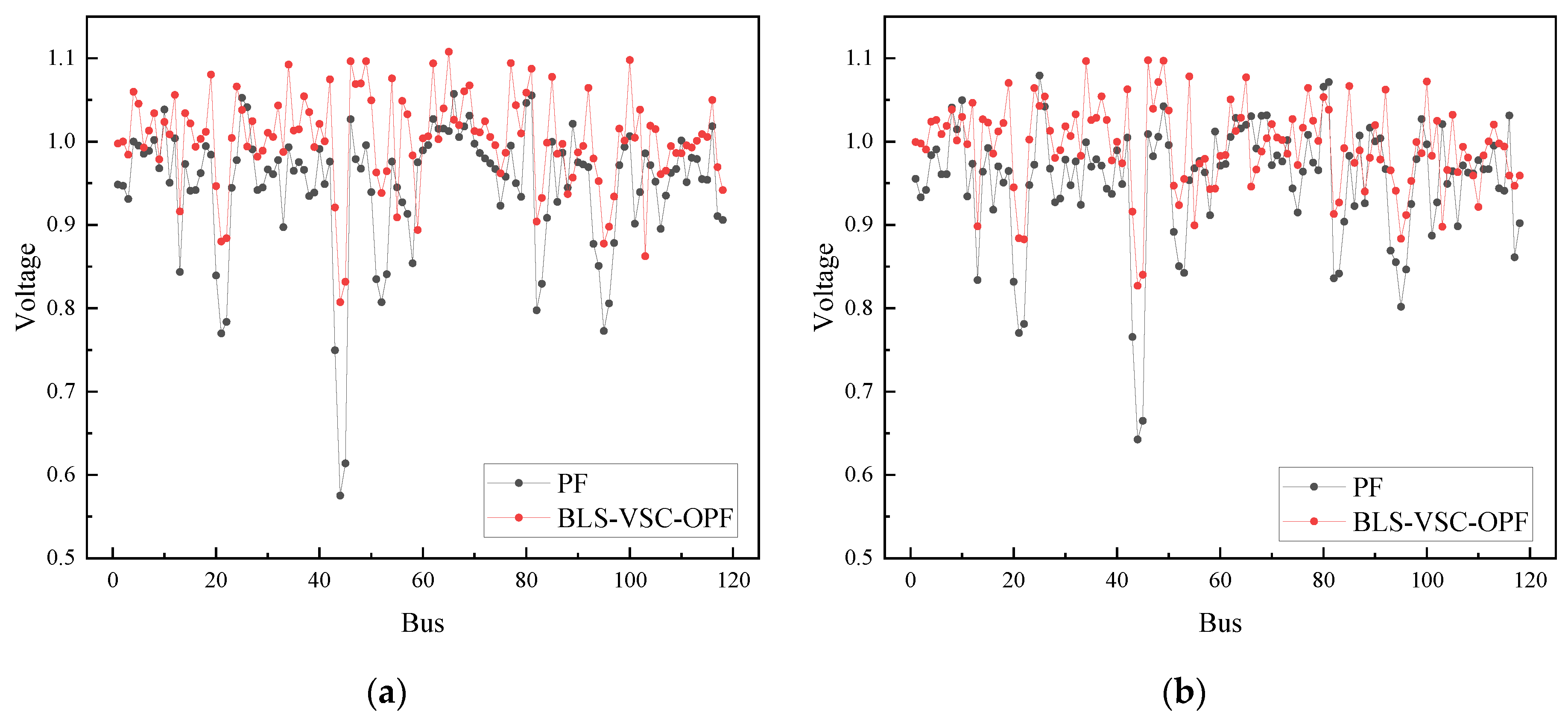
Similarly, taking Case2 and Case5 as examples, Figure 7 presents a comparison of the voltages before and after correction. It is worth noting that, in the IEEE-118 bus system, bus 44 experiences the weakest voltage. In Case2, the voltage of bus 44 is 0.5752 before correction. After correction by the BLS-VSC-OPF model, the voltage of this bus is increased to 0.8072. In Case5, the voltage of bus 44 is 0.6425 before correction, which is improved to 0.8269 after correction. Due to the large number of generators, their sensitivity and power output graphs have been omitted. Based on the analysis of simulation results from the two systems, it can be confidently concluded that the BLS-VSC-OPF model is applicable not only to the IEEE-30 bus system but also to complex systems like the IEEE-118 bus system. The model can effectively correct the L-index and improve the voltage stability of the system.

6.4. BLS-VSC-OPF Model for the 1047 Bus System

In order to demonstrate the compatibility of the BLS-VSC-OPF model with large systems, the model is applied to correct a set of operating modes in the 1047 bus system, comprising 152 generators, 164 transformers, 363 loads, and 1182 branches. The L-index threshold is established at 0.5 for this system. Prior to the correction, the actual L-index for the system stood at 0.7320, with the lowest voltage at 0.7784. Following correction, the L-index fell to 0.4775, and the minimum voltage increased to 0.9132. The results shown in

Table 10. Comparison of results before and after correction in the 1047 bus system.

	PF	BLS-VSC-OPF
Predicted value of L-index	0.7146	0.4971
Actual value of Lindex	0.7320	0.4775
Relative Error	2.38%	4.12%
Minimum Voltage	0.7784	0.9132

show that the BLS-VSC-OPF model still maintains a good correction ability in large systems.

6.5. Comparison of BLS-LPC Model and BLS-VSC-OPF Model

In order to demonstrate the superiority of the BLS-VSC-OPF model, the model is compared with the LPC model, which is commonly used in economic scheduling [34]. The BLS-LPC model is a linear model. The model mainly includes two parts: prediction and correction. Firstly, the BLS is used to predict the L-index of the system. When the L-index of the system is unqualified, the sensitivity of the L-index is calculated by the BLS and the perturbation method, and then the adjustment amount of the generator output is obtained by solving linear equations. Finally, the system is corrected to make the voltage return to a reasonable level. To enhance the correction capabilities of the BLS-LPC model, the correction effect of the PV nodes’ voltage with respect to the L-index is additionally considered. The model can be expressed as follows:

$$\min f(x)=a\cdot {\displaystyle \sum _{i\in S_G}\mathsf{\Delta }{P}_{Gi}^2}+b\cdot {\displaystyle \sum _{i\in S_G}\Delta V_{Gi}^2}$$

(19)

$$s.t.\{\begin{array}{c}\begin{array}{l}{P}_{Gi}^{min}\le P_{Gi0}+\Delta P_{Gi}\le P_{Gi}^{max}\\ V_{Gi}^{min}\le V_{Gi0}+\Delta V_{Gi}\le V_{Gi}^{\max }\end{array}\\ L_0+\Delta L\le L_{lim it}\\ {\displaystyle \sum _{i\in S_G}(C_{Pi}\Delta P_{Gi}+C_{Vi}}\Delta V_{Gi})=\Delta L\end{array}$$

(20)

where a and b are the weighted factors and are set to 0.9 and 0.1, respectively. ΔP_Gi, ΔV_Gi, and ΔL are the amounts of the adjustment, $L_{\lim it}$ is the threshold of the L-index, which is set to 0.5, and C_Pi and C_Vi are the sensitivities, which can be calculated in a similar way to Equation (14).

In the IEEE-30 bus system, the BLS-LPC model is used to correct the cases mentioned in Table 4, and the results are shown in

Table 11. Calibration results of BLS-LPC model in IEEE-30 bus system.

	Initial Value		First Correction		Second Correction
	L-Index	Minimum Voltage	L-Index	Minimum Voltage	L-Index	Minimum Voltage
Case1	0.9848	0.6261	0.5418	0.8643	0.4397	0.9641
Case2	0.9191	0.6467	0.5183	0.8728	0.4706	0.9174
Case3	0.8531	0.6761	0.5065	0.8841	0.4900	0.8993
Case4	0.8368	0.6876	0.5075	0.8961	0.4899	0.9122
Case5	0.7738	0.6999	0.4816	0.8956	/	/
Case6	0.7340	0.7245	0.4688	0.9153	/	/

. It can be seen that, if the L-index of the system is greater than the threshold, only one correction by the BLS-VSC-OPF model is necessary to bring the L-index back within the threshold, as shown in Table 4. However, in instances of poor voltage stability, due to nonlinear errors [34], the BLS-LPC model needs to be corrected several times to adjust the L-index to within the threshold, as demonstrated in Table 11.

After the second correction, the BLS-PCL model can meet the L-index requirements. It is worth noting that the threshold of the L-index is set to 0.5, and there is a certain distance between the L-index corrected by the BLS-LPC model and the threshold. Taking Case1 as an example, the system L-index is 0.9848 and the minimum voltage is 0.6261 before correction. After the second correction, the system L-index is 0.4397 and the minimum voltage is 0.9641. It is evident that the voltage is over-corrected by the BLS-LPC model, which causes the L-index to drop excessively. Although the overcorrection problem will not affect the stable operation of the system, it will lead to energy waste and economic loss.

Table 12. Comparison of ∑PG and ∑QG in IEEE-30 bus system.

	∑PGi/MW		∑QGi/Mvar
	BLS-VSC-OPF	BLS-LPC	BLS-VSC-OPF	BLS-LPC
Case1	575.53	599.56	296.09	309.70
Case2	552.92	583.81	308.16	333.57
Case3	544.91	579.24	300.15	327.73
Case4	580.51	612.73	300.17	325.74
Case5	568.93	592.03	316.85	334.65
Case6	550.32	568.51	299.67	311.47

compares the generator outputs of the BLS-VSC-OPF model and the BLS-LPC model after correction. The active power output and reactive power output of the BLS-VSC-OPF model are lower than those of the BLS-LPC model, meaning that the former has higher economic benefits.

Table 13. Comparison of correction results in IEEE-30 bus system.

	BLS-VSC-OPF			BLS-LPC
	Threshold	Actual L-Index	Relative Error	Threshold	Actual L-Index	Relative Error
Case1	0.5	0.4929	1.42%	0.5	0.4397	12.06%
Case2	0.5	0.5069	1.38%	0.5	0.4706	5.88%
Case3	0.5	0.5054	1.08%	0.5	0.4900	2.00%
Case4	0.5	0.5009	0.18%	0.5	0.4899	2.02%
Case5	0.5	0.5053	1.06%	0.5	0.4816	3.68%
Case6	0.5	0.5064	1.28%	0.5	0.4688	6.24%

shows the errors between the threshold and the actual L-index after the corrections of the BLS-VSC-OPF model and BLS-LPC model. When the BLS-VSC-OPF model is applied to correct, the error between the L-index and threshold is about 1%, with a maximum error of 1.42% and a minimum error of only 0.18%. In contrast, when the BLS-LPC model is employed, the error between the corrected L-index and the threshold is significantly larger, with the maximum error being as high as 12.06% and the minimum error being 2%. A detailed error comparison diagram is shown in Figure 8.

As described in the previous sections, the proposed BLS-VSC-OPF model is based on the classical OPF model, which includes the network topology information of the power system. The network topology describes the physical connections among the generators, transformers, lines, and loads in the system and plays a critical role in the state assessment of the power system [42]. With the support of network topology, the BLS-VSC-OPF method successfully establishes a complete system model, endowing it with excellent correction capabilities. As a result, the model can better capture the global information of the system, accurately determine the adjustment direction and amount of the generator, improve the efficiency of correction, and make the correction results closer to the expected value. By contrast, the BLS-LPC model is a linear correction control model which is framed by a system of linear equations. Therefore, when it comes to grasping the distance between the current system state and the target system state, the BLS-LPC model performs significantly worse than the BLS-VSC-OPF model.

In the BLS-VSC-OPF model, the controlled variables are the active power and reactive power of the generator. Among them, the reasonable allocation of reactive power is crucial for maintaining system voltage stability and addressing voltage issues [43]. Therefore, this model can effectively manage power allocation by adjusting the active power and reactive power of the generator, thereby improving the voltage stability. Even in complex IEEE-118 and 1047 bus systems, it can meet L-index requirements through a single correction, as shown in Table 9 and Table 10. However, the BLS-LPC method is based on the classical PF model, in which the reactive power of the generator is an uncontrollable variable. Therefore, the correction ability of this model has certain limitations. In the IEEE-118-bus system and the 1047 bus system, the model is unable to correct for the operation mode where the L-index exceeds the threshold. In conclusion, the BLS-VSC-OPF model offers superior economic benefits and correction ability compared to the BLS-LPC model.

7. Conclusions

In this paper, a BLS-VSC-OPF model is proposed to improve the voltage stability of systems. The assessment was performed on the IEEE-30, IEEE-118, and 1047 bus systems. The training and testing results show that the BLS has more than 95% accuracy in experimental systems, which satisfies the requirements of practical power systems. Secondly, the BLS is combined with the VSC-OPF model for the first time, which solves the problem of the complicated derivation process and difficult calculation of L-index sensitivity in the VSC-OPF model. Finally, we correct the operation mode of the L-index beyond the safe range by the BLS-VSC-OPF model. The corrected results show that, if the L-index of an operation mode exceeds the threshold, the model can correct the L-index to within the threshold. In addition, we compare the BLS-LPC model with the proposed model. In the IEEE-30 bus system, the proposed model requires fewer corrections, has a higher correction accuracy, and exhibits no over-correction phenomenon. In the IEEE-118 bus system and the 1047 bus system, the proposed model maintains a good correction ability while the BLS-LPC model cannot be corrected.

References

- Worku, M.Y. Recent Advances in Energy Storage Systems for Renewable Source Grid Integration: A Comprehensive Review. Sustainability 2022, 14, 5985. [Google Scholar] [CrossRef]
- Andersson, G.; Donalek, P.; Farmer, R.; Hatziargyriou, N.; Kamwa, I.; Kundur, P.; Martins, N.; Paserba, J.; Pourbeik, P.; Sanchez-Gasca, J.; et al. Causes of the 2003 Major Grid Blackouts in North America and Europe, and Recommended Means to Improve System Dynamic Performance. IEEE Trans. Power Syst. 2005, 20, 1922–1928. [Google Scholar] [CrossRef]
- Al-Shetwi, A.Q. Sustainable development of renewable energy integrated power sector: Trends, environmental impacts, and recent challenges. Sci. Total Environ. 2022, 822, 153645. [Google Scholar] [CrossRef] [PubMed]
- Modarresi, J.; Gholipour, E.; Khodabakhshian, A. A comprehensive review of the voltage stability indices. Renew. Sustain. Energy Rev. 2016, 63, 1–12. [Google Scholar] [CrossRef]
- Musirin, I.; Rahman, T.K.A. Novel fast voltage stability index (FVSI) for voltage stability analysis in power transmission system. In Proceedings of the Student Conference on Research and Development, Shah Alam, Malaysia, 17–17 July 2002; pp. 265–268. [Google Scholar]
- Moghavvemi, M.; Omar, F.M. Technique for contingency monitoring and voltage collapse prediction. IEEE Proc. Gener. Transm. Distrib. 1998, 145, 634–640. [Google Scholar] [CrossRef]
- Moghavvemi, M.; Faruque, M.O. Technique for assessment of voltage stability in ill-conditioned radial distribution network. IEEE Power Eng. Rev. 2001, 21, 58–60. [Google Scholar] [CrossRef]
- Milosevic, B.; Begovic, M. Voltage-stability protection and control using a wide-area network of phasor measurements. IEEE Trans. Power Syst. 2003, 18, 121–127. [Google Scholar] [CrossRef]
- Kessel, P.; Glavitsch, H. Estimating the Voltage Stability of a Power System. IEEE Trans. Power Deliv. 1986, 1, 346–354. [Google Scholar] [CrossRef]
- Lof, P.A.; Andersson, G.; Hill, D.J. Voltage stability indices for stressed power systems. IEEE Trans. Power Syst. 1993, 8, 326–335. [Google Scholar] [CrossRef]
- Althowibi, F.A.; Mustafa, M.W. Power system network sensitivity to Voltage collapse. In Proceedings of the 2012 IEEE International Power Engineering and Optimization Conference, Melaka, Malaysia, 6–7 June 2012; pp. 379–383. [Google Scholar]
- Chen, H.; Jiang, T.; Yuan, H.; Jia, H.; Bai, L.; Li, F. Wide-area measurement-based voltage stability sensitivity and its application in voltage control. Int. J. Electr. Power Energy Syst. 2017, 88, 87–98. [Google Scholar] [CrossRef]
- Tuglie, E.D.; Dicorato, M.; Scala, M.L.; Scarpellini, P. A corrective control for angle and voltage stability enhancement on the transient time-scale. IEEE Trans. Power Syst. 2000, 15, 1345–1353. [Google Scholar] [CrossRef]
- Zhihong, F.; Ajjarapu, V.; Maratukulam, D.J. A comprehensive approach for preventive and corrective control to mitigate voltage collapse. IEEE Trans. Power Syst. 2000, 15, 791–797. [Google Scholar] [CrossRef] [PubMed]
- Nahid Al, M.; Shazon, M.N.H.; Deeba, S.R.; Modak, S.R. A Frequency and Voltage Stability-Based Load Shedding Technique for Low Inertia Power Systems. IEEE Access 2021, 9, 78947–78961. [Google Scholar] [CrossRef]
- Ismail, B.; Wahab, N.I.A.; Othman, M.L.; Radzi, M.A.M.; Vijyakumar, K.N.; Naain, M.N.M. A Comprehensive Review on Optimal Location and Sizing of Reactive Power Compensation Using Hybrid-Based Approaches for Power Loss Reduction, Voltage Stability Improvement, Voltage Profile Enhancement and Loadability Enhancement. IEEE Access 2020, 8, 222733–222765. [Google Scholar] [CrossRef]
- Shokouhandeh, H.; Latif, S.; Irshad, S.; Ahmadi Kamarposhti, M.; Colak, I.; Eguchi, K. Optimal Management of Reactive Power Considering Voltage and Location of Control Devices Using Artificial Bee Algorithm. Appl. Sci. 2022, 12, 27. [Google Scholar] [CrossRef]
- Gu, C.; Ai, Q. Optimal Power Flow Considering Voltage Stability Constraints. Power Syst. Technol. 2006, 99, 29–34. [Google Scholar] [CrossRef]
- Zabaiou, T.; Dessaint, L.A. VSC-OPF based on line voltage indices for power system losses minimization and voltage stability improvement. In Proceedings of the 2013 IEEE Power & Energy Society General Meeting, Vancouver, BC, Canada, 21–25 July 2013; pp. 1–5. [Google Scholar]
- Liu, X.; Li, J.; Cheng, X.; Cao, L. A new method to determine optimal secure operating point of power system. Power Syst. Technol. 2005, 29, 56–60. [Google Scholar] [CrossRef]
- Cui, B.; Sun, X.A. A New Voltage Stability-Constrained Optimal Power-Flow Model: Sufficient Condition, SOCP Representation, and Relaxation. IEEE Trans. Power Syst. 2018, 33, 5092–5102. [Google Scholar] [CrossRef]
- Song, Y.; Liu, T.; Hou, Y. Voltage Stability Constrained Optimal Power Flow Considering PV-PQ Bus Type Switching: Formulation and Convexification. IEEE Trans. Power Syst. 2023, 39, 3336–3348. [Google Scholar] [CrossRef]
- Li, S.; Hou, J.; Yang, A.; Li, J. DNN-Based Distributed Voltage Stability Online Monitoring Method for Large-Scale Power Grids. Front. Energy Res. 2021, 9, 625914. [Google Scholar] [CrossRef]
- Hossain, R.R.; Huang, Q.; Huang, R. Graph Convolutional Network-Based Topology Embedded Deep Reinforcement Learning for Voltage Stability Control. IEEE Trans. Power Syst. 2021, 36, 4848–4851. [Google Scholar] [CrossRef]
- Zhu, L.; Luo, Y. Deep Feedback Learning Based Predictive Control for Power System Undervoltage Load Shedding. IEEE Trans. Power Syst. 2021, 36, 3349–3361. [Google Scholar] [CrossRef]
- Wang, T.; Liu, Y.; Qiu, G.; Ding, L.; Wei, W.; Liu, J. Deep learning-driven evolutionary algorithm for power system voltage stability control. Energy Rep. 2022, 8, 319–324. [Google Scholar] [CrossRef]
- Pan, X.; Chen, M.; Zhao, T.; Low, S.H. DeepOPF: A Feasibility-Optimized Deep Neural Network Approach for AC Optimal Power Flow Problems. IEEE Syst. J. 2023, 17, 673–683. [Google Scholar] [CrossRef]
- Nadimi-Shahraki, M.H.; Taghian, S.; Mirjalili, S.; Abualigah, L.; Abd Elaziz, M.; Oliva, D. EWOA-OPF: Effective Whale Optimization Algorithm to Solve Optimal Power Flow Problem. Electronics 2021, 10, 2975. [Google Scholar] [CrossRef]
- Ahmed, M.K.; Osman, M.H.; Shehata, A.A.; Korovkin, N.V. A Solution of Optimal Power Flow Problem in Power System Based on Multi Objective Particle Swarm Algorithm. In Proceedings of the 2021 IEEE Conference of Russian Young Researchers in Electrical and Electronic Engineering (ElConRus), Moscow, Russia, 26–29 January 2021; pp. 1349–1353. [Google Scholar]
- Duong, T.L.; Nguyen, N.A.; Nguyen, T.T. A Newly Hybrid Method Based on Cuckoo Search and Sunflower Optimization for Optimal Power Flow Problem. Sustainability 2020, 12, 5283. [Google Scholar] [CrossRef]
- Siano, P.; Cecati, C.; Yu, H.; Kolbusz, J. Real Time Operation of Smart Grids via FCN Networks and Optimal Power Flow. IEEE Trans. Ind. Inform. 2012, 8, 944–952. [Google Scholar] [CrossRef]
- Owerko, D.; Gama, F.; Ribeiro, A. Optimal Power Flow Using Graph Neural Networks. In Proceedings of the ICASSP 2020–2020 IEEE International Conference on Acoustics, Speech and Signal Processing (ICASSP), Barcelona, Spain, 4–8 May 2020; pp. 5930–5934. [Google Scholar]
- Singh, M.K.; Kekatos, V.; Giannakis, G.B. Learning to Solve the AC-OPF Using Sensitivity-Informed Deep Neural Networks. IEEE Trans. Power Syst. 2022, 37, 2833–2846. [Google Scholar] [CrossRef]
- Yang, Y.; Huang, Q.; Li, P. Online prediction and correction control of static voltage stability index based on Broad Learning System. Expert Syst. Appl. 2022, 199, 117184. [Google Scholar] [CrossRef]
- Yang, Y.; Fang, H.; Yang, L. Predictive Analysis and Correction Control of CCT for a Power System Based on a Broad Learning System. Sustainability 2023, 15, 9155. [Google Scholar] [CrossRef]
- Luo, L.; Wang, J.; Zhou, S.; Lou, G.; Sun, J. A broad learning-based state estimation method for power system. Energy Rep. 2022, 8, 1227–1235. [Google Scholar] [CrossRef]
- Chen, C.L.P.; Liu, Z. Broad Learning System: An Effective and Efficient Incremental Learning System Without the Need for Deep Architecture. IEEE Trans. Neural. Netw. Learn Syst. 2018, 29, 10–24. [Google Scholar] [CrossRef] [PubMed]
- Gong, X.; Zhang, T.; Chen, C.L.P.; Liu, Z. Research Review for Broad Learning System: Algorithms, Theory, and Applications. IEEE Trans. Cybern. 2022, 52, 8922–8950. [Google Scholar] [CrossRef] [PubMed]
- Wei, H.; Li, B.; Hang, N.; Liu, D.; Wen, J.; Sasaki, H. An Analysis of Interior Point Theory for Large-Scale Hydrothermal optimal power flow problems. Proc. CSEE 2003, 4, 9–12. [Google Scholar] [CrossRef]
- Wei, H.; Li, B.; Hang, N.; Liu, D.; Wen, J.; Sasaki, H. An Implementation of Interior Point Algorithm for Large-Scale Hydro-Thermal Optimal Power Flow Problem. Proc. CSEE 2003, 6, 13–18. [Google Scholar] [CrossRef]
- Zabaiou, T.; Dessaint, L.A.; Kamwa, I. A comparative study of VSC-OPF techniques for voltage security improvement and losses reduction. In Proceedings of the 2014 IEEE PES General Meeting | Conference & Exposition, National Harbor, MD, USA, 27–31 July 2014; pp. 1–5. [Google Scholar]
- Gotti, D.; Amaris, H.; Larrea, P.L. A Deep Neural Network Approach for Online Topology Identification in State Estimation. IEEE Trans. Power Syst. 2021, 36, 5824–5833. [Google Scholar] [CrossRef]
- Qin, W.; Wang, P.; Han, X.; Du, X. Reactive Power Aspects in Reliability Assessment of Power Systems. IEEE Trans. Power Syst. 2011, 26, 85–92. [Google Scholar] [CrossRef]
Figure 1.
Structure of BLS.
Figure 2.
The basic framework of the BLS-VSC-OPF model.
Figure 3.
(a) Actual and predicted values of BLS for IEEE-30 bus system; (b) actual and predicted values of BLS for IEEE-118 bus system; (c) actual and predicted values of BLS for 1047 bus system.
Figure 4.
(a) Sensitivity of the L-index to the active power of the generator in Case2; (b) sensitivity of the L-index to the reactive power of the generator in Case2; (c) comparison of voltage levels of two models in Case2.
Figure 5.
(a) Sensitivity of the L-index to the active power of the generator in Case4; (b) sensitivity of the L-index to the reactive power of the generator in Case4; (c) comparison of voltage levels of two models in Case4.
Figure 6.
(a) Sensitivity of the L-index to the active power of the generator in Case6; (b) sensitivity of the L-index to the reactive power of the generator in Case6; (c) comparison of voltage levels of two models in Case6.
Figure 7.
(a) Comparison of voltage levels of two models in Case2; (b) comparison of voltage levels of two models in Case5.
Figure 8.
Comparison of the errors of the two correction models in IEEE-30 bus system.