
Resource Scheduling Optimization of Fresh Food Delivery Porters Considering Ambient Temperature Variations

School of Business, Renmin University of China, Beijing 100872, China
*
Author to whom correspondence should be addressed.
Sustainability 2024, 16(9), 3624; https://0-doi-org.brum.beds.ac.uk/10.3390/su16093624
Submission received: 8 March 2024
/
Revised: 4 April 2024
/
Accepted: 10 April 2024
/
Published: 26 April 2024
(This article belongs to the Section Energy Sustainability)
Abstract
:In the context of an evolving socio-economic landscape and rising living standards, the online market for fresh products, encompassing fruits, vegetables, meats, dairy, and eggs, has seen substantial growth, necessitating sophisticated logistics for e-commerce home delivery. This study tackles the distinct challenges of fresh product delivery, which demand rigorous adherence to climate conditions and product mix during transport, significantly influencing the operational strategies and scheduling of delivery platforms. To address these challenges, a comprehensive mathematical model was developed to optimize fresh food home delivery scheduling, focusing on reducing spoilage rates and accommodating the dynamic impact of environmental temperature changes. The model posits assumptions of a consistent and ample supply of fresh goods, standard initial quality loss, and efficient porter assignment for multi-category order combinations. It introduces three objective functions, targeting the minimization of fresh food loss, maximization of customer satisfaction, and reduction of distributor costs. The efficacy of the model and its genetic-algorithm-based solution method was assessed through numerical analysis and case studies, illustrating that the model enhances delivery efficiency and service quality across varying temperature conditions. This substantiates the critical role of environmental temperature management in optimizing fresh food delivery, offering a robust framework for advancing logistical operations in the perishable goods sector and ensuring quality and efficiency in fresh food e-commerce delivery.
1. Introduction
1.1. Research Background
The development of digital technology for traditional retail has transformed fresh food home delivery in China, introducing a mix of online ordering and offline delivery that improves access to fresh products. Since EGo Fresh started in 2005, the fresh food e-commerce sector has evolved significantly, with major platforms like Alibaba and JingDong driving innovations in digital and management practices [1,2].
The industry has diversified since 2014, developing models like front warehouses and community group purchasing to meet various consumer needs, pushing the fresh food e-commerce market toward a projection of 6.8 trillion yuan by 2025 [3]. The pandemic further accelerated this growth, as home quarantine measures and heightened health and safety concerns increased online shopping and demand for quality fresh products. In response, the Chinese government has prioritized food safety, issuing policies to enhance cold chain logistics and promote logistics informatization [4]. The 14th Five-Year Plan focuses on upgrading cold chain standards for food and pharmaceuticals, aiming to improve food safety and consumer quality standards [5].
However, delivering fresh products at home is challenging due to the need for maintaining freshness and transportation efficiency. Traditional delivery methods can lead to spoilage, delays, and the reliance on delivery porters, who lack advanced cold chain facilities and can increase losses and costs, affecting consumer satisfaction and the efficiency of fresh food e-commerce businesses. This study, therefore, concentrates on analyzing how ambient temperature affects the quality of fresh food delivery, aiming to optimize delivery service efficiency and enhance consumer satisfaction in the fresh food e-commerce sector.
1.2. Literature Review
In academic discourse, the emphasis has been on the influence of supply chain networks and contemporary technological advancements in enhancing the freshness quality of perishable products, safeguarding food safety, and achieving consumer satisfaction. Todorovic et al. (2018) analyzed sustainable strategies in short food supply chains, emphasizing the integration of business modeling and digital technologies to enhance supply chain efficiency and sustainability [6]. Biuki, Kazemi, and Alinezhad (2020) developed an integrative model for the sustainable configuration of perishable product supply chain networks, considering factors like location, routing, and inventory management to boost efficiency across the food, pharmaceutical, and healthcare sectors [7]. Sinha and Anand (2020) introduced a model that employs an advanced bacterial foraging algorithm to optimize the perishable product supply chain, effectively managing resource allocation during critical scenarios, such as military rescue operations, and underscoring the significance of adept supply chain management in preserving product quality [8]. Additionally, the role of technological tools has been accentuated in scholarly works. Ben-Daya et al. (2020) examined how Internet of Things (IoT) technology can augment the traceability and monitoring of perishable goods to enhance freshness, diminish waste, and ensure food safety [9]. Benke and Tomkins (2017) investigated the effects of drone delivery technology on home delivery services for fresh food products through empirical field trials and simulation analysis [10]. Haji et al. (2020) delved into various technologies within the perishable food supply chain, such as tracking and monitoring systems, aiming to ameliorate logistics and distribution quality and efficiency, curtail wastage, and augment product freshness [11]. Furthermore, Pal and Kant (2020) explored the contributions of smart sensing, communication, and control technologies to the perishable food supply chain, emphasizing the necessity of real-time monitoring, temperature regulation, and logistical optimization to ensure the freshness and safety of food products [12].
In terms of consumer satisfaction with fresh home delivery services, studies such as those by Qin et al. (2019) highlight the critical factors for success in fresh food home delivery, including cost control, customer satisfaction, and sustainability [13]. Wang et al. (2021) and Lim et al. (2021) provide insights into consumer preferences, underscoring the importance of safety, quality, convenience, delivery speed, and effective error resolution as key drivers of satisfaction [14,15]. The study by Porat et al. (2018) revealed the causes and magnitude of fruit and vegetable losses in the retail and home segments through empirical research and data analysis, pointing out that environmental and social factors such as storage conditions, consumption habits, and lack of knowledge have a direct impact on the rate of loss of fresh products [16].
1.3. Research Significance
Most of the existing studies focus on temperature regulation within cold chain logistics for agricultural produce, with scant attention given to the direct effects of temperature fluctuations during the actual distribution phase. Notably, the role of delivery porters in the fresh food home delivery sector presents distinct characteristics compared to conventional large-scale cold chain logistics operations. This study seeks to elucidate the mechanisms through which ambient temperature variations affect the deterioration rates of fresh commodities, impacting the quality and efficiency of fresh food home delivery, with a particular focus on delivery porters as pivotal logistical entities.
Building upon the foundational studies of Ndraha et al. (2019), who illuminated the direct impact of distribution temperature on the quality of fresh products [17], and Ji Shoufeng et al. (2023), who developed a model that integrates the perishability of fresh products with logistical expenses, this research proposes a dynamic scheduling optimization framework [18]. This framework is designed to accommodate ambient temperature fluctuations, aiming to refine distribution routes and timings to preserve the freshness and quality of products. By integrating ambient temperature considerations and the specific traits of various fresh product categories (such as meats, seafood, fruits, and vegetables) into a comprehensive scheduling model, this study intends to bolster operational efficiency and consumer satisfaction within the fresh food distribution sector. The proposed model introduces a freshness loss rate index as a critical metric, offering a novel perspective for optimizing scheduling decisions that are responsive to ambient temperature dynamics.
This study’s contributions are poised to enhance the resilience and quality standards of the fresh food distribution industry, fostering improved consumer satisfaction and aligning with the strategic objective of augmenting food safety and consumer quality standards.
2. Scenario Analysis of Fresh Product Home Delivery
Fresh home delivery encompasses a diverse range of products, including fruits, vegetables, meats, dairy, seafood, and frozen goods, each with specific preservation needs. The complexity of managing these varied requirements demands precise control over refrigeration and insulation to maintain freshness, alongside ensuring timely deliveries and intact packaging. This necessitates a sophisticated order management and scheduling system that can adapt to real-time environmental conditions and unforeseen changes.
The primary challenge in this sector is balancing product quality, delivery speed, and cost efficiency. The unpredictable nature of environmental conditions significantly impacts delivery quality. For instance, delivering temperature-sensitive items like ice cream or yogurt in high midday heat requires not only rapid transit but also enhanced cooling strategies. This situation demands delivery personnel capable of navigating extreme conditions and using specialized equipment to preserve product integrity.
2.1. Demand: Influencing Factors in the Process of Fresh Product Home Delivery
2.1.1. Ambient Temperature Environments
Ambient temperature is pivotal in the storage and distribution of fresh food. High moisture and nutrient content in items like fruits, vegetables, meats, and seafood make them susceptible to microbial growth, which is significantly influenced by temperature. Higher temperatures facilitate rapid microbial proliferation, hastening spoilage and reducing the food’s shelf life. Consequently, managing temperature is essential during distribution to slow microbial activity, including methods like refrigeration for meats and seafood. Conversely, certain produce, such as tropical fruits, may require specific temperature ranges to avoid damage.
In the current literature, Aung and Chang (2014) stated in their study that improper temperature control can negatively affect food quality by leading to increased loss of vitamin C and food spoilage [19]. Wu and Hsiao (2021) stated that proper temperature control slows down microbial growth and reduces the risk of food spoilage and decay [20]. Some studies have pointed out the different effects of environmental weather elements such as temperature or humidity on various types of fresh products. Likotrafiti et al. (2013) examined the growth potential of Listeria monocytogenes in different ready-to-eat fruit products, highlighting how storage temperature significantly affects the microbial growth and thus the spoilage rate, which varies across different fruit types [21]. Kroft et al. (2022) investigated the effects of temperature on the growth and survival of Listeria monocytogenes in a variety of whole and fresh-cut fruits and vegetables during storage, demonstrating how different types of fresh products respond to temperature changes [22].
These studies underscore that the impact of temperature on spoilage and quality degradation vary among different types of fresh products, with specific temperature and humidity conditions affecting each category’s shelf life and safety. In this way, Figure 1 can be derived to plot the negative effect of temperature on the quality of fresh products based on existing research and common sense, while the mechanism of this effect receives the moderating effect of the fresh products category.
Building on this, the study introduces a novel mathematical indicator, the “weather coefficient”, , to quantify short-term ambient temperature trends. The weather coefficient is derived from the temperature’s rate of change over time, reflecting potential shifts towards warmer or cooler conditions. Mathematically, the weather coefficient can be defined as follows:
where denotes temperature and time; positive and negative values of signify increasing and decreasing temperature trends, respectively. This coefficient provides a broad indicator of temperature dynamics, valuable for short-term forecasts, long-term seasonal predictions, and cross-regional temperature trend analysis.
Incorporating weather coefficient into fresh home delivery models can significantly refine transportation and storage strategies for temperature-sensitive goods. By anticipating temperature fluctuations, distributors can tailor their logistics plans to maintain optimal conditions for fresh products, potentially necessitating additional protective measures during critical periods. Consequently, the use of not only minimizes the risk of spoilage but also enhances overall transportation efficiency by enabling more informed decision-making regarding insulation and cooling strategies.
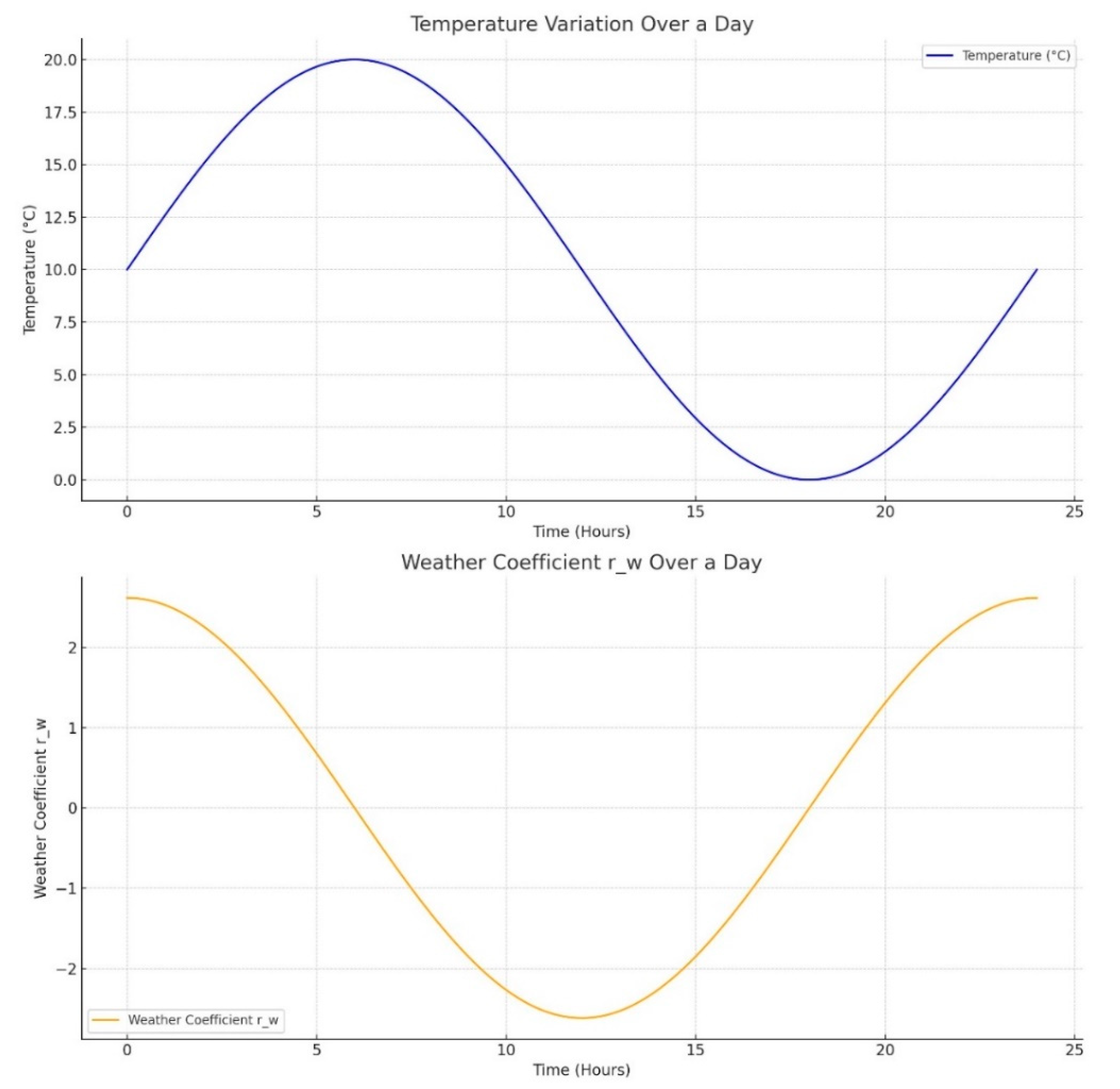
As illustrated in Figure 2, a scholarly tailored visualization of diurnal temperature fluctuations and the associated weather coefficients is integral to the logistical management of fresh food distribution. This self-constructed graph is predicated on the widely recognized principle that diurnal temperatures follow a sinusoidal oscillation due to the Earth’s axial rotation and the consequent rhythmic patterns of solar irradiation. The illustration has been expressly generated to encapsulate typical temperature variations over a daily cycle and the resultant weather coefficients . The diagram is bifurcated into two segments: the upper segment displays a sinusoidal trajectory, projecting the anticipated ambient temperature shifts within a day, while the lower section of the diagram is derived through the discrete differentiation of the sinusoidal curve presented in the upper section, capturing the incremental rate of temperature change at successive points throughout the day. This calculated derivative conveys the weather coefficients reflecting the intensity and velocity of temperature shifts, which are instrumental for strategic planning in the logistics of perishable goods transport.
Analyzing the weather coefficient curve reveals that positive values occur during temperature increases (e.g., morning when the sun rises) while negative values are noted as temperatures decrease (e.g., evening when the sun sets). These coefficients offer a clear, intuitive method for assessing temperature trends, crucial for managing temperature-sensitive tasks such as fresh home delivery. By leveraging this insight, planners can make informed decisions regarding temperature control strategies and operational adjustments.
2.1.2. Variability in Fresh Food Categories
Fresh products encompass a broad spectrum of items, each with unique preservation challenges, sensitivity, and shelf life. These distinctions manifest not only in their physical and chemical properties but also in how consumers perceive and judge quality. Individual preferences vary widely, with consumers valuing different aspects of fresh products, such as freshness, taste, and packaging integrity.
To gain insight into consumer quality preferences across various fresh food categories, we analyzed extensive online review data, identifying key dimensions that shape consumer evaluations. For instance, our analysis revealed that fruit and vegetable quality assessments often hinge on perishability and sensitivity; meat and frozen seafood evaluations prioritize freshness and preservation levels; packaging and refrigeration efficiency are critical for ice cream and dairy products; and freshness and sensitivity are paramount for aquatic and live poultry products.
This analytical approach not only deepens our understanding of consumer preferences but also informs recommendations for product classification, packaging design, and delivery methods in fresh food home delivery. For highly perishable items, enhanced packaging and expedited shipping are advisable, whereas maintaining optimal temperature and humidity is crucial for items requiring freshness. By tailoring strategies to these insights, distributors can more effectively satisfy consumer demands, elevating service quality, customer loyalty, and competitive edge.
Hence, as delineated in Table 1, consumers prioritize different attributes across fresh food categories, leading to the distinction of two specific metrics for assessing fresh food loss: perishability () and vulnerability (). Perishability () gauges the speed at which fresh products degrade in unsuitable conditions, while vulnerability () measures the likelihood of damage during handling.
Given these attributes, we can establish a fresh food perishability index, , correlating with the characteristics of each fresh food category. This index reflects the condition of fresh products during delivery to a specific user, focusing solely on the product’s inherent loss potential due to its physical and chemical properties, independent of external environmental factors. The index, , as a fusion of perishability () and vulnerability (), offers a nuanced view of each category’s preservation challenges and susceptibility to damage.
To simplify model construction while accommodating varying consumer priorities, this study adopts expert scoring to define the characteristics of fresh food categories within the index . Mathematically, it is represented as follows:
where and are the perishability and vulnerability scores for category m, and and denote the respective weights of these attributes. This formula effectively combines perishability and vulnerability scores, weighted by their importance, to quantitatively evaluate fresh product loss rates, enhancing prediction accuracy for distribution-related wastage and its impact on consumer satisfaction. By employing this method, distributors can better forecast and manage product wastage, refining delivery strategies to boost consumer satisfaction.
2.2. Supply: Impact of Porter Attributes on Delivery Scheduling
Effective fresh food delivery hinges on minimizing loss rates and maximizing efficiency to enhance customer satisfaction and reduce operational costs for the provider. To achieve this, delivery services must strategically allocate third-party porters, considering the nature of various fresh food items and anticipated weather conditions. Key to this strategy is the assessment of porter attributes and their available delivery equipment, ensuring alignment with the specific requirements of each order.
Porters today are outfitted with specialized equipment for diverse delivery scenarios. For instance, those equipped with refrigeration units are invaluable for transporting temperature-sensitive items during hot weather. Selecting porters with advanced cooling technology is crucial for maintaining the freshness of highly perishable goods. Additionally, a porter’s delivery speed and order acceptance rate are crucial factors influencing overall delivery effectiveness and product preservation.
Assuming consistent product quality, the delivery service’s role is to meticulously match orders to porters based on product characteristics and current weather, optimizing service quality and cost-efficiency. As shown in Table 2, we give an example of the porter attributes. Consider a hypothetical porter with specific attributes: load capacity , impacting the volume of deliveries; average speed , which influences delivery timeliness and temperature-sensitive product loss (faster speeds mitigate ambient temperature effects, reducing spoilage); equipment cooling or insulating capabilities , crucial for maintaining product quality in transit; and the cost per delivery , reflecting labor expenses only.
By analyzing and selecting porters based on these attributes, a delivery service can assign orders to the most suitable personnel. For example, orders requiring swift delivery of refrigerated items should be assigned to quick porters with efficient cooling equipment. Conversely, for products less affected by temperature, choosing porters with greater load capacity but lower costs may be preferable. This strategic deployment of porters, tailored to the nuances of each order, not only elevates the transport quality and efficiency for fresh goods but also secures a competitive edge for the delivery service in a highly competitive market. An illustrative table of porter attributes is presented below for reference:
3. Fresh Product Home Delivery Porter Scheduling Analysis and Metrics Characterization
3.1. Fresh Food Loss Rate
Managing the loss rate is pivotal in fresh food home delivery, directly impacting consumer satisfaction and operational efficiency. This study focuses on two critical aspects to enhance the delivery scheduling model: the perishability and vulnerability of fresh food categories and the variation in ambient temperatures during transit. The perishability attributes indicate the potential for loss across different fresh product types, recognizing that some items may spoil quickly in high temperatures or suffer damage from handling. Ambient temperature changes, especially during distribution and the duration of transport, also play a significant role in affecting loss rates.
By integrating these considerations, distributors can more precisely forecast and reduce wastage of fresh goods, thus elevating service quality and strengthening market position.
3.1.1. Category Characteristics of Fresh Orders
Fresh products, encompassing fruits, vegetables, aquatic items, dairy, meats, and prepared foods, exhibit distinct perishability and vulnerability characteristics. Perishability describes the tendency of items like fruits, meats, and fish, which require refrigeration, to spoil or degrade. Vulnerability, on the other hand, refers to the risk of damage during transportation for delicate items such as premium fruits and dairy products. Assessing these aspects allows for an understanding of attrition rates across different product categories.
To quantify these rates, we introduce an index, , reflecting the wastage rate for a specific category based on its perishability characteristics. This index, , combines perishability, vulnerability, and other relevant factors to determine each product’s loss potential during delivery.
Considering additional perishability attributes beyond perishability () and vulnerability (), such as moisture level, compressive strength, and oxidation resistance, we incorporate these into the category characteristic index as a weighted sum:
where represents the weight of the attribute and its score. This formulation reflects the multifaceted nature of perishability and provides a comprehensive assessment of wastage potential.
For an order containing multiple fresh product categories, the composite index is derived by integrating individual category indices , accounting for interactions among different categories within an order. The overall characteristic index for order n, , is calculated as follows:
where m is the number of categories in the order, the score of the category on the attribute, and a weighting factor reflecting the importance of each category in the order.
This comprehensive approach not only evaluates the loss potential of individual categories but also the collective impact when combined in an order. By providing a quantitative framework to predict and manage the overall attrition rate, aids distributors in identifying and mitigating risks in fresh food delivery, enhancing service quality and efficiency.
3.1.2. Impact of Ambient Temperature Changes on Fresh Food Delivery
Understanding the loss rate in fresh food delivery requires consideration of both the characteristics of the fresh food itself and the complex influence of ambient temperature changes during transportation. The weather coefficient , representing the trend of ambient temperature at the delivery time , and the transportation duration , from the distribution center to the consumer, are critical factors.
The weather coefficient indicates whether the temperature is likely to rise or fall at a specific time . A positive suggests an increasing temperature trend, typically seen in the morning, while a negative indicates a decreasing trend, common in the afternoon. The rate of fresh food loss is thus influenced by the issuance time of the order, , and the weather coefficient . During periods of stable high or low temperatures, becomes zero, implying that the impact of weather on loss rates can be disregarded, focusing instead on the inherent perishability of the food.
The relationship between the weather coefficient , transportation duration , and the resultant loss rate is not linear. Shorter can mitigate losses even under rising temperatures, while longer durations in less favorable conditions increase spoilage risk.
To quantify the effect of ambient temperature on fresh food loss rates accurately, we introduce a new coefficient termed the “coefficient of ambient temperature change impact on fresh food loss rate”, denoted as (). This coefficient, , encapsulates the combined effects of delivery timing, transportation length, and temperature trends on loss rates, providing a nuanced view of environmental influences on fresh food logistics.
This model enables a more precise estimation of temperature-related losses, enhancing the scheduling and management of fresh food deliveries to minimize spoilage and optimize service quality.
3.1.3. Detailed Analysis of Fresh Food Loss Rate in Home Delivery
Incorporating discussions on fresh food order categories and environmental temperature fluctuations during delivery, this study develops a composite indicator for the fresh food loss rate This rate is influenced by two primary factors: the impact of fresh food category characteristics within an order on loss rate, denoted as , and the effect of ambient temperature changes, represented by . The factor accounts for how the perishability and fragility of different fresh food categories affect overall product loss. In contrast, combines transportation duration and dispatch time into a function that captures ambient temperature change impacts on loss rates. The fresh food loss rate is expressed as follows:
For instance, an order’s fresh food loss rate will depend on the collective perishability traits of the included categories () and the ambient temperature variations (). Specifically, necessitates consideration of weather conditions at the delivery time and anticipated transportation length. For example, orders dispatched during hot conditions with lengthy transportation times imply a higher and, thus, increased loss risk. Conversely, rapid deliveries in mild conditions would lower the risk.
Consider a hypothetical scenario with five different order types, as shown in Table 3, each having unique category characteristics indices , and four potential dispatch times. The interplay between these indices and corresponding weather coefficients () influences the overall fresh food loss rate as demonstrated in the table below:
This model considers both key factors—the perishable characteristics of the fresh food category and ambient temperature changes—to calculate . By precisely assessing these elements, distributors can enhance their fresh food delivery services, reducing wastage, boosting customer satisfaction, and maintaining competitive advantage.
3.2. Measuring Consumer Satisfaction in Fresh Food Delivery
Consumer satisfaction, a critical metric for fresh food delivery success, influences brand reputation and loyalty. Satisfaction hinges on delivery timeliness and the condition of fresh products upon arrival. Shorter transportation times () typically boost satisfaction by ensuring freshness, while extended delivery can diminish food quality, affecting the consumer experience. Moreover, the fresh food delivery loss rate (), indicating the percentage of products lost or degraded during transit, directly impacts the quality and quantity of products received by consumers, further influencing satisfaction levels.
Assuming an initial product quality (q) consistent across all categories upon entering the distribution center, the fresh food loss rate () reduces quality from this baseline, affecting overall consumer satisfaction. Satisfaction () is thus influenced by transportation duration () and the loss rate ().
We consider two scenarios for calculating satisfaction, incorporating the concept of an expected delivery time window:
- (i)
- On-time delivery. Here, satisfaction is a function inversely related to transportation duration, where p is the duration–satisfaction coefficient (within [−1, 0]):
- (ii)
- Off-schedule delivery (early or late). Quality deterioration continues over time, raising negotiation costs with the service provider. In such cases, satisfaction is modeled as follows:where is a parameter within [−1, 0], is the delivery completion time by porter to user , and and represent the start and end of the consumer’s expected delivery window, respectively.
Therefore, the consumer satisfaction function is detailed as follows:
3.3. Analyzing Total Distributor Costs
In the unique domain of fresh food home delivery, distributors are confronted with various cost components that are vital for maintaining service quality and competitiveness. These costs include cold chain technology expenses, transportation and labor costs, and compensation for any loss of freshness. Each cost directly influences the service’s quality and efficiency, playing a pivotal role in sustaining customer satisfaction.
These are as follows:
- (1)
- Technology costs (). These costs cover all expenses related to preserving the quality of fresh products, ensuring minimal wastage. This encompasses the upkeep and operation of refrigeration systems, transport equipment, and technical support. Technology costs are influenced by the porter’s equipment, where porters equipped with advanced refrigeration systems, indicating higher technology attributes, incur greater expenses for the distributor.
- (2)
- Transportation Cost (). This represents the porter’s labor costs per delivery. Porters with better load capacity can transport more goods per trip, potentially reducing the number of trips but incurring higher labor costs. However, this capability typically leads to lower fresh food loss rates and heightened consumer satisfaction due to decreased loss and enhanced timeliness.
- (3)
- Compensation cost for freshness loss (). This cost arises when consumer satisfaction falls below a certain threshold, necessitating compensation for damages or delays, such as refunds for severely damaged goods or delayed deliveries. Faster porter speeds can diminish transportation times, reducing loss and, consequently, compensation costs. Conversely, longer transport times increase the per-unit time loss rate (), raising the compensation expenses, which can be modeled as follows:where is a parameter reflecting the proportion of compensation cost in the total expense.
Combining these costs allows for a comprehensive distributor cost model, facilitating strategic decision-making and optimization. This model aids in understanding the interplay between different costs and their impact on the efficiency and economy of delivery services. Through this multifaceted cost analysis, distributors can finely tune the balance between cost and service quality, aiming for sustainability and profitability.
For a specific porter, the cost incurred by the delivery service is as follows:
Hence, the proposed total cost model for distributors is expressed as follows:
In order to simplify the research problem, this study builds a model based on the following assumptions: (1) the supply of fresh food suppliers to the distributor is sufficient and continuous; (2) when the distributor obtains fresh goods from the supplier, the initial loss value of fresh goods is the same fixed value, and the porter will not cause loss of fresh quality before obtaining the goods for departure; (3) the distributor assigns only one order combination to a porter at a time, which contains multiple categories of fresh products, i.e., the order combination is similar to the distribution provider’s secondary combination of user orders to maximize distribution efficiency.
4. Model Building and Numerical Analysis
In formulating this delivery scheduling model, the goal is to select appropriate porters based on order characteristics to minimize transport loss rates, maximize service satisfaction, and minimize costs. Below Table 4 is a detailed description of the parameters and variables used in the model.
This study develops a multi-layered, time-windowed distribution scheduling optimization model focusing on fresh food categories. The optimization objectives encompass three main areas: (1) ensuring timely deliveries and maintaining fresh food quality and quantity, thus boosting consumer satisfaction; (2) minimizing distributor costs to enhance profitability; (3) lowering the fresh food loss rate to uphold overall logistics and distribution quality, safeguarding food safety.
4.1. Objective Function
The model comprises three objective functions, outlined from Equation (1) to Equation (3), aimed at minimizing the fresh food loss rate, maximizing consumer service satisfaction, and reducing the distributor’s total costs, respectively.
4.2. Constraints
This study addresses the Vehicle Routing Problem with Time Windows (VRPTW), focusing on delivering goods from distribution centers to customers with varying demand levels within specific timeframes. The objective is to optimize routes for distribution personnel to fulfill customer demands efficiently under constraints, achieving minimal distance and cost.
The VRPTW aims to balance multiple objectives under the following constraints:
- (1)
- Time window constraint: all deliveries must be completed within the designated time windows. Any deviation by a porter from a customer’s specified time window () contributes to the overall tally of time window violations, which represents the cumulative number of instances where porters have failed to meet the time window constraint.
- (2)
- Porter’s cargo capacity constraint: at any given moment, the combined load of all porters should not exceed the capacity constraints (). This means that the sum of all capacity violations, representing the total fresh food resources at the distributor’s center, should be zero.
Considering the “last-mile” delivery to users, the aggregate capacity/order volume for all porters cannot surpass the total inventory available, given the following constraints:
where represents the total capacity constraints exceeded during the delivery of fresh food, and denotes the aggregate time window constraints breached by all orders. indicates the time a porter takes to deliver an order from the distribution center to the specified user. The term refers to the duration within a user ’s designated delivery time window. Equation (4) applies constraints to the cost variables identified in Equation (3), while Equation (5) imposes limitations on the satisfaction metrics outlined in Equation (2).
4.3. Algorithms
This model tackles a multi-objective optimization problem with inherent constraints, typifying an NP-hard problem. Given the complexity, exact algorithms are impractical due to their extensive computational demand. Hence, heuristic methods, particularly stochastic algorithms, are preferred for their ability to escape local optima and strive for a global solution. Techniques like Simulated Annealing, Tabu Search, Genetic Algorithms, and Ant Colony Optimization are utilized for their effectiveness [23,24]. Among these, the Genetic Algorithm (GA) stands out for its applicability to integer programming problems involving 0–1 variables. Its advantages include not requiring function continuity or differentiation, possessing excellent global optimization capabilities [25], and exhibiting self-organization, adaptation, and learning traits [26,27], making it especially suitable for this model.
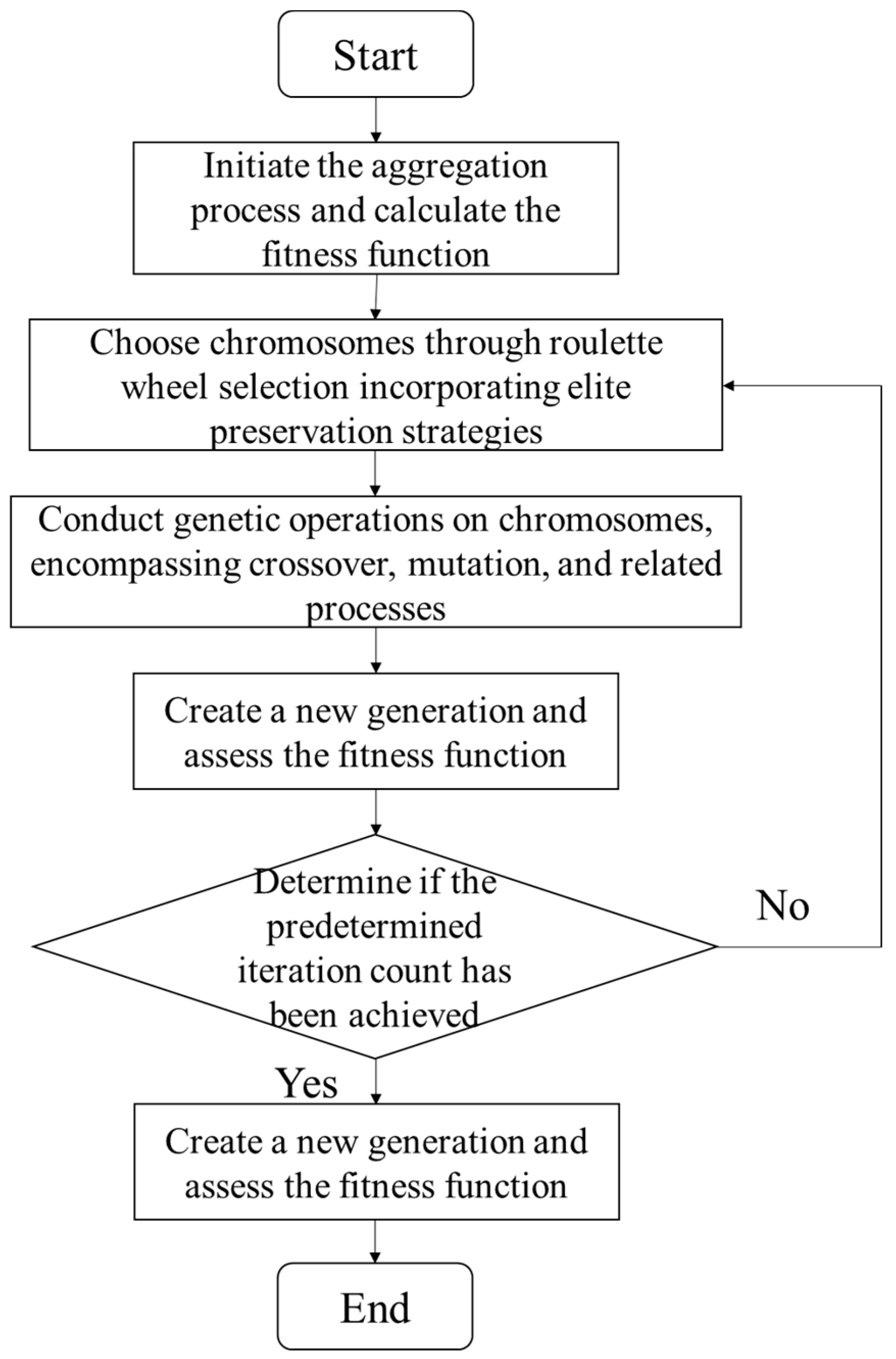
The GA process involves the following, as shown in Figure 3:
- (1)
- Initialization. The algorithm initiates with a population of potential scheduling strategies, where each solution delineates a specific dispatch of porters to fresh product orders contingent on their perishability levels. In this study, real-number encoding is utilized to generate a set of potential solutions. The chromosome length is determined by the total decision variables, , indicating the selection of fresh product categories by porter for order The population size is set at 200, providing a broad range of solutions.
- (2)
- Genetic operations This phase encompasses several operations to evolve the population:
- Crossover (probability of 0.9): this operation fuses the genetic information from pairs of parent solutions to produce offspring, aiming to amalgamate beneficial traits for an effective match of porters to orders based on perishability.
- Mutation (probability of 0.6): this phase involves a series of processes to dynamically evolve the population, including crossover, mutation, blending with the parental population, and assessing the fitness of each individual.
- Evaluation: following crossover and mutation, the offspring form a new population that is assessed alongside the initial parental group, creating a diverse genetic pool that balances stability and innovation. Mirroring the natural selection process, the evaluation phase is crucial for ensuring that superior individuals prevail. In this context, each chromosome is assigned a fitness value reflecting its effectiveness in meeting the objective function. The higher the fitness value, the higher the likelihood of that individual being carried over to the subsequent generation. This selection is predicated on the fitness values, where individuals are chosen to be parents for the next generation based on their demonstrated fitness.
- (3)
- Selection: upon calculating the fitness values for all chromosomes, selection is conducted using strategies like roulette-wheel and elitism, ensuring a balanced propagation of advantageous traits. The algorithm selects the most apt solutions from the merged population, emphasizing those schedules where porters are optimally matched with orders based on perishability, thus minimizing spoilage and maximizing logistical efficiency.
- (4)
- Termination: the algorithm iterates through these genetic operations until it achieves 300 iterations, a predefined threshold ensuring a comprehensive exploration of the optimal scheduling solutions under the specified perishability considerations.
The objective functions, addressing both minimization and maximization challenges, are converted to minimization problems for simplicity. The conversion is as follows:
To account for the scale differences between objective functions, they are made dimensionless, enabling the conversion of a multi-objective problem into a singular objective function by assigning appropriate weights [28,29]. These weights adapt based on the decision-making context. For instance, increased emphasis on the fresh food loss rate might occur following frequent customer complaints, while strict cost control measures would prioritize minimizing delivery costs.
A linear weighting approach amalgamates the three objective functions into a singular minimization problem. Assuming weights , ′, and (satisfying + ′ + = 1), the aggregated objective function Z can be formulated as follows:
Therefore, linearly integrating the transformed objective functions, the model’s objective function simplifies to the following:
To manage constraints, a penalty function is introduced, transforming constrained issues into unconstrained ones by incorporating a term proportional to the violation degree into the objective function. Utilizing a quadratic penalty function,
Here, β signifies a substantial positive penalty factor, and represents the constraint. If ≤ 0, constraints are met, and the penalty is null; otherwise, a positive penalty reflects constraint violations. For the identified constraints, the penalty function can be detailed as follows:
Incorporating these penalty terms modifies each objective function as follows:
- For :
- For :
- For :
The penalty factor β is chosen to ensure adherence to constraints throughout the optimization, with the penalty function and parameter settings significantly influencing the solution’s efficacy and outcome quality.
4.4. Numerical Study
Utilizing the algorithmic framework discussed, a simulation was performed to evaluate porter scheduling in various delivery scenarios, considering distinct fresh food categories and ambient temperature variations. As shown in Table 5, the simulation features four orders with unique category characteristics, each exhibiting a varied loss rate due to the combined effects of fresh food type and temperature. These orders are denoted by to , while five available porters are represented as to . Each porter is assigned to deliver these orders based on their specific attributes, such as speed, capacity, insulation conditions, and cost. For simplicity, all parameters were normalized.
This table integrates fresh food category traits with the ambient temperatures faced during delivery, setting the basis for calculating order attrition rates, denoted as to . An optimized delivery strategy is then crafted based on each porter’s attributes.
Table 6 presents a genetic-algorithm-based optimization example for a delivery service. The specific numerical values presented in this table are randomly generated; however, the range and scope of these values were determined through consultations with industry experts and internal stakeholders to ascertain the pertinent dimensions and parameters for delivery service performance. This table details the performance metrics for different porters ( to ) handling orders with varying fresh food loss rates ( to ). The metrics include product wear rate, service satisfaction, and total service cost, providing a comprehensive view of each porter’s effectiveness in delivering the orders. Product wear rate indicates the percentage of products likely to deteriorate or spoil during delivery. For instance, porter handling order has a wear rate of 0.85, suggesting a high likelihood of product spoilage, potentially due to longer delivery times or inadequate storage conditions. Service satisfaction measures the customer’s satisfaction level with the delivery service, factoring in timeliness, product condition upon arrival, and overall service experience. For example, porter for order scores 0.85 in service satisfaction, implying a very positive customer reception, possibly due to exceptional delivery performance. Total service cost reflects the economic efficiency of the delivery service, encompassing fuel, labor, and other logistical expenses. A lower score indicates a more cost-effective service. For instance, porter with order shows a total cost of 0.43, denoting efficient delivery at a lower cost.
The table facilitates a multi-dimensional evaluation of the delivery service, where decision-makers can analyze and select the optimal porter for each order type based on a balance of wear rate, satisfaction, and cost. For example, while porter may have a high product wear rate for orders, this is counterbalanced by high service satisfaction and low total service cost, suggesting a trade-off between the risk of product spoilage and high customer satisfaction with cost efficiency. Next, we will use a genetic algorithm to solve this numerical study case.
The optimization problem aims to balance the minimization of fresh loss rate, maximization of consumer satisfaction, and minimization of distributor costs, with weights of 0.4, 0.4, and 0.2, respectively. In this study, the optimization problem is framed as a multi-objective endeavor, prioritizing the minimization of fresh loss rate and the maximization of consumer satisfaction, each assigned a weight of 0.4, alongside the minimization of distributor costs with a weight of 0.2. This equal prioritization of fresh loss and consumer satisfaction underscores the business’s strategic focus on mitigating perishable goods’ spoilage while enhancing client contentment. The allocation of weights is a strategic decision, reflecting a nuanced balance between maintaining product integrity and ensuring high customer satisfaction. It stems from an in-depth analysis of the business model, wherein reducing perishable losses and achieving high customer satisfaction are seen as crucial drivers of operational success and market competitiveness. The chosen weights, indicative of the business’s operational focus, are substantiated by empirical insights gained through extensive industry research and direct consultations with companies engaged in perishable goods management. This approach is supported by the literature, such as the study by Liang et al. (2023), which discusses the importance of balancing objectives like fresh loss minimization and consumer satisfaction in multi-objective optimization for perishable goods delivery [30], and the work by Bortolini et al. (2016) that examines the design of multi-modal fresh food distribution networks, emphasizing the need for a balanced consideration of cost and service quality [31]. These references highlight a deliberate strategy to optimize both product quality and consumer experience in the competitive landscape, confirming the relevance of the chosen weight distribution in reflecting real-world operational priorities.
Using MATLAB_2021b, the algorithm parameters were meticulously determined through extensive iterative processes, resulting in a population size of 200, a crossover probability of 0.9, a mutation probability of 0.6, and a total of 300 iterations. These parameters were validated for their efficacy and appropriateness in achieving optimal algorithm performance. After 50 algorithm runs, the average iteration time was 1.77 s, indicating high computational efficiency. Upon convergence, the optimal fitness value averaged 1.22822, demonstrating stable results and robust algorithm performance. The best scheduling yielded objective function values of 0.35 (fresh loss rate), 2.43 (consumer satisfaction), and 0.36 (distributor cost). Figure 4 and Figure 5 depict the convergence of model fitness and objective functions, with Table 7 outlining the optimal scheduling strategy.
The optimal scheduling outlined in Table 7 demonstrates the strategic selection of porters for orders characterized by varying fresh food loss rates. This approach highlights a meticulous pairing of porters’ unique capabilities with the specific demands of the orders.
Specifically, based on this table of results, we can examine an example of a real-world scenario. In an urban setting characterized by a robust demand for fresh products, a delivery firm specializing in perishable goods navigates the challenge of minimizing food spoilage whilst adhering to stringent delivery timelines. The optimal scheduling strategy, as delineated in Table 7, encapsulates the firm’s strategic acumen in allocating porters to orders based on varying rates of fresh food loss, thereby optimizing service delivery. The firm’s operational tactics are exemplified in the allocation of porter to orders with loss rates and . This selection is predicated on ’s demonstrated proficiency in managing items with high perishability, such as ripe berries and leafy greens. The porter’s vehicle, equipped with advanced cooling technologies, ensures the freshness of these goods during transit. Additionally, ’s adept navigation through the city’s traffic network facilitates the expedited delivery of these perishables, minimizing time in transit and, hence, the potential for spoilage. For orders exhibiting a loss rate , the company strategically selects porter , who excels in servicing peripheral urban areas where longer transit times prevail. ’s expertise in durable packaging and rural route navigation makes him ideally suited for transporting slightly more resilient perishables, such as whole grains and root vegetables, ensuring their freshness upon delivery. In addressing the most susceptible orders with loss rate , the firm entrusts porter , renowned for handling temperature-sensitive produce like exotic fruits. leverages specialized containment systems that maintain consistent internal conditions, counteracting external temperature variances. His comprehensive understanding of the city’s microclimates informs the meticulous planning of delivery routes, circumventing areas prone to thermal anomalies.
This targeted scheduling strategy, founded on a deep understanding of both porter attributes and order needs, aims to enhance delivery efficiency and service quality. By judiciously matching orders with the most appropriate porters, the strategy not only curtails wastage and elevates customer satisfaction but also boosts the delivery service’s overall operational efficiency. This meticulous resource allocation ensures optimal service performance, leveraging advanced models and algorithms to address the challenges of fresh home delivery under variable environmental temperatures effectively.
5. Discussion
5.1. Sensitive Analysis
Fresh food home delivery reflects the burgeoning prosperity of the new retail industry, attracting significant attention from the logistics sector, consumers, and broader societal stakeholders. However, the inherent challenges, particularly the stringent requirements for storage and transportation to preserve product quality, cannot be overlooked. Traditional distribution methods often fall short in addressing these demands, with the dynamic changes in ambient temperature posing a notable challenge to maintaining fresh product quality and transportation efficiency—a factor commonly underestimated.
In this section, the machine learning random forest method is utilized as a surrogate model (or proxy model) to conduct sensitivity analysis on the original study and to assess the outcomes using the SHAP framework. While random forests are typically employed for predictive or classification endeavors, in this context, they serve as a proxy to emulate the genetic algorithm’s operational dynamics. This surrogate modeling facilitates a nuanced understanding of the impact of various input variables on the genetic algorithm’s output (Jiang Wang et al., 2020; S.A. Naghibi et al., 2017; H Norouzi et al., 2021) [32,33,34].
Within the ambit of multi-objective optimization modeling, the construction of a surrogate model coupled with SHAP analysis necessitates a sequence of methodical procedures. Initially, this encompasses data generation, then it transitions into surrogate modeling, and finally culminates in conducting SHAP analysis, as depicted in Figure 6.
- Data generation. This process initiates with the operation of a multi-objective optimization model, such as a genetic algorithm, under varied parameter configurations or weightings to produce a comprehensive dataset. This dataset comprises input parameters and their corresponding optimization outcomes, the latter representing the values derived from the multi-objective optimization endeavor.
- Surrogate modeling. Subsequently, a machine learning model, akin to a random forest, gradient boosting machine, or neural network, is selected based on its congruence with the optimization model’s dynamics, serving as a surrogate model. This model aims to mimic the behavioral attributes of the original multi-objective optimization framework, trained on the dataset generated earlier, with the input parameters as features and the optimization outcomes as target variables.
- Conducting SHAP analysis. Upon model training, the SHAP library aids in quantifying the individual impact of each input feature on each optimization objective’s output. Through SHAP value summary and dependency plots, the critical input parameters and their effects on the optimization results are elucidated.
In this section, we aligned with the genetic algorithm execution detailed in the primary study, especially referencing the algorithm’s data input in Table 6, to interpret and leverage the genetic-algorithm-generated data. Utilizing MATLAB, we exported the iterative data from the genetic algorithm into a CSV file, forming the basis for the subsequent SHAP analysis.
- Descriptive statistics. Our dataset comprises 60,000 data entries, each including variables such as Iteration, Feature 1, Feature 2, Feature 3, Feature 4, and Fitness Value. The following Table 8 is the descriptive statistics chart for this dataset.
The Iteration column records each iteration of the genetic algorithm, serving as a marker to trace the algorithm’s progression and iterative dynamics, albeit not directly employed as a predictive feature in the random forest model. Columns like Feature 1, Feature 2, … Feature 4 represent decision variables optimized within the genetic algorithm framework. These variables are treated as input features in the random forest model, facilitating the construction of the model and prediction of the objective function value. Fitness Value enables the simulation and analysis of the optimization process of the genetic algorithm.
- 2.
- Meaning of feature values. In this context, Features 1 to 4 are assigned specific business implications, signifying the loss rates of different orders and pivotal decision variables in the multi-objective optimization model. For instance, Feature 1 correlates with the loss rate or related parameters of the first order, providing a quantified depiction of its loss scenario. This not only reflects the actual physical loss but also encompasses the comprehensive impact of order loss on aspects like cost, time, and customer satisfaction. Similarly, Feature 2 is associated with the second order’s loss rate or parameters, unveiling the characteristics and performance metrics of that order within the optimization process executed by the genetic algorithm. The same applies to Features 3 and 4. These features vividly display the loss scenarios of fresh product orders under the combined influence of weather conditions such as temperature, humidity, ventilation, delivery timing and duration by the delivery personnel, and the internal variety of fresh products within the orders. Utilizing the dataset extracted from the genetic algorithm, these features simulate varying business scenarios, affording the model an opportunity to explore the optimization landscape. In the random forest model, these features are harnessed as input variables with the aim of predicting an aggregated objective variable related to the order, such as total loss rate, distributor cost, and key business performance indicators like customer satisfaction. Through this approach, the random forest model elucidates how different order features collectively impact the optimization objectives, offering a crucial perspective for a deeper understanding of the genetic algorithm’s optimization process.
We employed the SHAP function in Python 3.11.5 to analyze a random forest surrogate model, with X_train representing the input features and y_train the output of the optimization model. The random forest regressor served as the surrogate model, instantiated in Python as shap.TreeExplainer. Once the surrogate model was trained, we proceeded to generate summary plots of the SHAP values. Figure 7, entitled SHAP summary plot, characterizes the impact of various features on the predictive output within a machine learning model. The SHAP values are based on the Shapley values from cooperative game theory and provide a rigorously unbiased metric on the contribution of predictions. They calculate each feature’s contribution through its average marginal contribution [35].
In Figure 7, the horizontal axis displays the SHAP values, quantifying how these feature values influence the model’s output. Negative SHAP values indicate that a feature decreases the model prediction, whereas positive SHAP values signify an increase in predicted values. As Figure 7 shows, Feature 1 exhibits a relatively wide distribution of SHAP values, indicating significant variability in its impact on model output across different instances. Features 2, 4, and 3 predominantly show a propensity towards the positive direction, suggesting they generally exert a positive influence on model output. Notably, the majority of SHAP values for Features 2 and 4 are positive, hinting that higher values of these features tend to increase the prediction outcome. In contrast, Feature 3 has a minimal impact, with its SHAP values clustering near zero, signifying a relatively lower influence on the model’s output.
5.2. Model for Combined Fresh Product Loss Rate Considering Other Weather Conditions
Building upon the previous discourse on ambient temperature, this section broadens the scope to an integrated loss rate for fresh products. The loss rate is governed by a complex interplay of various factors such as temperature, humidity, and ventilation through nonlinear and dynamic interactions. For instance, high humidity may accelerate the degradation and weight reduction of certain types of fresh products, particularly under optimal temperature conditions or inadequate ventilation. Initially, our investigation was solely concentrated on the impact of ambient temperature and time duration. Therefore, to evaluate the preservation status of fresh products more precisely during delivery, we advocate for the amalgamation of these weather elements into a comprehensive metric known as the integrated loss rate. This facilitates a more thorough depiction of the risk of loss for fresh products during transportation, and our preliminary model remains relevant for subsequent solution processes.
The integrated loss rate transcends the mere cumulative average of individual factors like temperature, humidity, and ventilation. It rather considers these factors in unison, assessing the overall loss rate from a systemic perspective. This integrated loss rate embodies a multi-tiered, multi-dimensional evaluation system. Practically, it is imperative to consider the interplay and potential conflicts among various weather elements, as well as the exponential effects of their collective impact, thus precluding the simplistic assignment of weights. Incorporation of the elasticity coefficient method, an economic tool for gauging the influence of variations in one indicator on another, might be beneficial. Hirschberg, Lye, and Slottje (2008) examined inferential methods for estimating elasticity, contributing to a deeper comprehension of demand sensitivity and elasticity within economic models [36]. Another study by Chattoe, Saam, and Möhring (1997) addressed the issues and prospects of sensitivity analysis in the social sciences, specifically highlighting the applicability of the elasticity coefficient in quantifying the impact of variable changes within models [37]. The quantification method for the elasticity coefficient is expressed as , where represents the rate of change in a specific weather condition and signifies the change in the integrated loss rate caused by this weather condition element at the same moment.
When multiple weather factors, including temperature, humidity, and ventilation, are considered concurrently, the elasticity coefficient of each weather element, , is defined as , where ranges between 0 and 1 ( [0, 1]) and belongs to the set , representing the quantified dimensions of weather conditions. The term denotes the weight of the impact of different weather elements on the integrated loss rate, calculated based on their respective elasticity coefficients to ensure that their contribution to the integrated loss rate is proportional to their relative change. This can be computed as . Here, the denominator represents the sum of the elasticity coefficients of all weather elements, ensuring that the sum of all equals 1, thereby facilitating the accurate allocation of weights.
For all weather elements, the model construction adheres to the methodology outlined in Section 3, which addresses the modeling of ambient temperature. This approach involves defining the instantaneous state of weather elements, such as humidity and ventilation, at the departure time of the delivery personnel, assessing whether conditions like increasing humidity or improved ventilation prevail. The initial loss rate, , remains applicable to the integrated loss rate model, signifying the baseline loss rate of the fresh product orders without accounting for the influence of weather factors. This rate is influenced by the departure time and the category of fresh products. In this context, the integrated loss rate model further contemplates the characteristics of fresh product categories within each order, acknowledging that different categories are affected distinctly by temperature, humidity, and ventilation. The considerations for temperature fluctuations presented in Section 3.1.2 are now extended to encompass all weather elements.
Referring to the principal study, the effect of departure time and transportation duration on fresh product orders, initially denoted as , is here considered as for all weather factors. Incorporating elasticity coefficients and weights into the computation of the integrated loss rate engenders a more dynamic and realistic model that mirrors actual conditions. Following the discussion, the integrated loss rate can be articulated as , where represents the foundational loss rate unaffected by weather elements and acts as the loss adjustment coefficient for each specific weather element, reflecting its actual impact on the loss of the fresh products.
Based on this integrated loss rate model, subsequent efforts can be directed towards employing the solution algorithm developed in this study to optimize the scheduling of delivery personnel for fresh products. This approach facilitates a strategic allocation of delivery resources, ensuring that perishable goods are transported efficiently while minimizing the risk of spoilage and loss during transit.
6. Conclusions
Fresh food home delivery reflects the burgeoning prosperity of the new retail industry, attracting significant attention from the logistics sector, consumers, and broader societal stakeholders. However, the inherent challenges, particularly the stringent requirements for storage and transportation to preserve product quality, cannot be overlooked. Traditional distribution methods often fall short in addressing these demands, with dynamic changes in ambient temperature posing a notable challenge to maintaining fresh product quality and transportation efficiency—a factor commonly underestimated.
In conclusion, this study delves into the impact of ambient temperature on the quality of fresh food distribution, uniquely capturing fresh food distribution attributes against the backdrop of ambient temperature and the demand for specific categories of products, establishing a core metric for evaluating fresh food wastage rates.
This study developed a multi-objective fresh product delivery scheduling optimization mathematical model, focusing on core factors directly linked to fresh product distribution. The model introduces three competing optimization goals: timely delivery to ensure product quality and customer satisfaction, cost minimization for distributor profitability, and reduced fresh product loss rate to maintain overall logistics quality and food safety. Utilizing a genetic algorithm for its global search capabilities, the model addresses the complexities of the multi-objective optimization problem effectively. Simulation results demonstrated the model’s robustness and the algorithm’s efficiency, offering optimal scheduling strategies that reduce loss and enhance customer satisfaction, thereby improving overall delivery service efficiency. In addition, this study continues to validate the effectiveness of the model using a machine learning random forest alternative model as a sensitivity test. The study also contemplates an integrated model that encompasses weather elements such as temperature, humidity, and ventilation, rendering the model more comprehensively applicable to real-world scenarios.
This study provides a comprehensive framework for assessing and optimizing fresh product delivery services, marking a significant theoretical and methodological contribution to cold chain logistics and intelligent distribution systems. However, future research should address the study’s limitations, such as refining temperature fluctuation modeling and extending the model’s applicability to various geographic and seasonal contexts. Additionally, developing more efficient algorithms and conducting empirical studies will be crucial for enhancing the model’s practical utility and validating its effectiveness in real-world applications.
Author Contributions
Writing—original draft, Z.S.; writing—review & editing, J.Y.; project administration, J.Y. All authors have read and agreed to the published version of the manuscript.
Funding
This research received no external funding.
Institutional Review Board Statement
Not applicable.
Informed Consent Statement
Not applicable.
Data Availability Statement
Data are contained within the article.
Acknowledgments
The authors would like to thank the anonymous reviewers and editors, whose valuable comments and corrections improved this work substantially.
Conflicts of Interest
The authors declare no conflicts of interest.
References
- iResearch Consulting Group. 2021 China Fresh E-Commerce Industry Research Report. Available online: https://report.iresearch.cn/report_pdf.aspx?id=3776 (accessed on 18 May 2021).
- Yunlian Research Institute. Secrets of Mainstream Fresh Food Platforms Revealed: Yiguo, Daily Fresh, and Fruit Day. Available online: https://zhuanlan.zhihu.com/p/43312689 (accessed on 31 August 2018).
- Titanium Media. From Yiguo Fresh to Daily Fresh, from Hema Fresh to Dmall. Available online: https://new.qq.com/rain/a/20220725A0532Z00 (accessed on 5 July 2022).
- The General Office of the State Council. Opinions on Accelerating the Development of Cold Chain Logistics to Ensure Food Safety and Promote Consumption Upgrade, Document No. [2017] 29. Available online: https://www.gov.cn/gongbao/content/2017/content_5191695.htm (accessed on 13 April 2017).
- The General Office of the State Council. Notice on Issuing the “14th Five-Year Plan” for Cold Chain Logistics Development, Document No. [2021] 46. Available online: https://www.gov.cn/zhengce/2021-12/14/content_5660638.htm (accessed on 14 December 2021).
- Todorovic, V.; Maslaric, M.; Bojic, S.; Jokic, M.; Mircetic, D.; Nikolicic, S. Solutions for More Sustainable Distribution in the Short Food Supply Chains. Sustainability 2018, 10, 3481. [Google Scholar] [CrossRef]
- Biuki, M.; Kazemi, A.; Alinezhad, A. An integrated location-routing-inventory model for sustainable design of a perishable products supply chain network. J. Clean. Prod. 2020, 260, 120842. [Google Scholar] [CrossRef]
- Sinha, A.K.; Anand, A. Optimizing supply chain network for perishable products using improved bacteria foraging algorithm. Appl. Soft Comput. 2020, 86, 105921. [Google Scholar] [CrossRef]
- Ben-Daya, M.; Hassini, E.; Bahroun, Z.; Banimfreg, B.H. The role of internet of things in food supply chain quality management: A review. Qual. Manag. J. 2020, 28, 17–40. [Google Scholar] [CrossRef]
- Benke, K.; Tomkins, B. Future food-production systems: Vertical farming and controlled-environment agriculture. Sustain. Sci. Pract. Policy 2017, 13, 13–26. [Google Scholar] [CrossRef]
- Haji, M.; Kerbache, L.; Muhammad, M.; Al-Ansari, T. Roles of technology in improving perishable food supply chains. Logistics 2020, 4, 33. [Google Scholar] [CrossRef]
- Pal, A.; Kant, K. Smart sensing, communication, and control in perishable food supply chain. ACM Trans. Sens. Netw. 2020, 16, 1–41. [Google Scholar] [CrossRef]
- Qin, G.; Tao, F.; Li, L. A vehicle routing optimization problem for cold chain logistics considering customer satisfaction and carbon emissions. Int. J. Environ. Res. Public Health 2019, 16, 576. [Google Scholar] [CrossRef]
- Wang, M.; Wang, Y.; Liu, W.; Ma, Y.; Xiang, L.; Yang, Y.; Li, X. How to achieve a win–win scenario between cost and customer satisfaction for cold chain logistics? Phys. A Stat. Mech. Appl. 2021, 566, 125637. [Google Scholar] [CrossRef]
- Lim, M.K.; Li, Y.; Song, X. Exploring customer satisfaction in cold chain logistics using a text mining approach. Ind. Manag. Data Syst. 2021, 121, 2426–2449. [Google Scholar] [CrossRef]
- Porat, R.; Lichter, A.; Terry, L.A.; Harker, R.; Buzby, J. Postharvest losses of fruit and vegetables during retail and in consumers’ homes: Quantifications, causes, and means of prevention. Postharvest Biol. Technol. 2018, 139, 135–149. [Google Scholar] [CrossRef]
- Ndraha, N.; Sung, W.C.; Hsiao, H.I. Evaluation of the cold chain management options to preserve the shelf life of frozen shrimps: A case study in the home delivery services in Taiwan. J. Food Eng. 2019, 242, 21–30. [Google Scholar] [CrossRef]
- Ji, S.-f.; Liu, H.-y.; Zhao, P.-y.; Ji, T.-t. Model and Algorithm of Dynamic Inventory Replenishment Based on Physical Internet. Chin. J. Manag. Sci. 2023, 31, 205–214. Available online: http://www.zgglkx.com/EN/10.16381/j.cnki.issn1003-207x.2020.0768 (accessed on 5 March 2024).
- Aung, M.M.; Chang, Y.S. Traceability in a food supply chain: Safety and quality perspectives. Food Control 2014, 39, 172–184. [Google Scholar] [CrossRef]
- Wu, J.Y.; Hsiao, H.I. Food quality and safety risk diagnosis in the food cold chain through failure mode and effect analysis. Food Control 2021, 120, 107501. [Google Scholar] [CrossRef]
- Likotrafiti, E.; Smirniotis, P.; Nastou, A.; Rhoades, J. Effect of Relative Humidity and Storage Temperature on the Behavior of Listeria monocytogenes on Fresh Vegetables. J. Food Saf. 2013, 33, 545–551. [Google Scholar] [CrossRef]
- Kroft, B.; Gu, G.; Bolten, S.; Micallef, S.A.; Luo, Y.; Millner, P.; Nou, X. Effects of temperature abuse on the growth and survival of Listeria monocytogenes on a wide variety of whole and fresh-cut fruits and vegetables during storage. Food Control 2022, 137, 108919. [Google Scholar] [CrossRef]
- Wang, M.; Yao, J. Intertwined supply network design under facility and transportation disruption from the viability perspective. Int. J. Prod. Res. 2023, 61, 2513–2543. [Google Scholar] [CrossRef]
- Xu, L.; Yao, J. Supply Chain Scheduling Optimization in an Agricultural Socialized Service Platform Based on the Coordination Degree. Sustainability 2022, 14, 16290. [Google Scholar] [CrossRef]
- Li, X.; Jiang, H.; Gu, J. Design of intelligent fresh food logistics terminal with internet of things under new retail mode. Comput. Appl. Softw. 2021, 38, 23–28. [Google Scholar] [CrossRef]
- Blue Snap. Research on the influencing factors of customer-perceived service quality of fresh food delivery based on web crawler technology. Logist. Sci. Technol. 2022, 45, 68–71. [Google Scholar] [CrossRef]
- Kumar, N.; Shanker, K. A Genetic Algorithm for FMS Part Type Selection and Machine Loading. Int. J. Prod. Res. 2000, 38, 3861–3887. [Google Scholar] [CrossRef]
- Lu, C.; Kou, J. QoS optimization of large-scale web service portfolio based on multi-objective multi-attribute decision making. Chin. J. Manag. 2018, 15, 586–597. [Google Scholar]
- Yang, Y.; Yao, J. Resource integration optimization of senior care service platform based on service model facilitation depth carving. Chin. J. Manag. 2020, 17, 725–733. [Google Scholar]
- Liang, X.; Wang, N.; Zhang, M.; Jiang, B. Bi-objective multi-period vehicle routing for perishable goods delivery considering customer satisfaction. Expert Syst. Appl. 2023, 220, 119712. [Google Scholar] [CrossRef]
- Bortolini, M.; Faccio, M.; Ferrari, E.; Gamberi, M.; Pilati, F. Fresh food sustainable distribution: Cost, delivery time, and carbon footprint three-objective optimization. J. Food Eng. 2016, 174, 56–67. [Google Scholar] [CrossRef]
- Wang, J.; Yan, W.; Wan, Z.; Wang, Y.; Lv, J.; Zhou, A. Prediction of permeability using random forest and genetic algorithm model. Comput. Model. Eng. Sci. 2020, 125, 1135–1157. [Google Scholar] [CrossRef]
- Naghibi, S.A.; Ahmadi, K.; Daneshi, A. Application of support vector machine, random forest, and genetic algorithm optimized random forest models in groundwater potential mapping. Water Resour. Manag. 2017, 31, 2761–2775. [Google Scholar] [CrossRef]
- Norouzi, H.; Moghaddam, A.A.; Celico, F.; Shiri, J. Assessment of groundwater vulnerability using genetic algorithm and random forest methods (case study: Miandoab plain, NW of Iran). Environ. Sci. Pollut. Res. 2021, 28, 39598–39613. [Google Scholar] [CrossRef]
- Heuillet, A.; Couthouis, F.; Díaz-Rodríguez, N. Collective Explainable AI: Explaining Cooperative Strategies and Agent Contribution in Multiagent Reinforcement Learning with Shapley Values. IEEE Comput. Intell. Mag. 2022, 17, 59–71. [Google Scholar] [CrossRef]
- Hirschberg, J.G.; Lye, J.N.; Slottje, D.J. Inferential methods for elasticity estimates. J. Econom. 2008, 147, 299–315. [Google Scholar] [CrossRef]
- Chattoe, E.; Saam, N.J.; Möhring, M. Sensitivity Analysis in the Social Sciences: Problems and Prospects. In Tools and Techniques for Social Science Simulation; Suleiman, R., Troitzsch, K.G., Gilbert, N., Eds.; Springer: Berlin/Heidelberg, Germany, 2000. [Google Scholar] [CrossRef]
Figure 1.
Temperature–fresh product quality influence mechanism diagram. Drawn by the authors.

Figure 2.
Diurnal temperature variation and associated weather coefficients for fresh food distribution logistics. Upper panel: a sinusoidal curve representing typical ambient temperature changes over a 24 h period. Lower panel: derived weather coefficients calculated through discrete differentiation of the temperature curve. Both visualizations were self-generated using Python by the authors for this study.

Figure 3.
Genetic algorithm programming process.

Figure 4.
Convergence results of the model adaptation.

Figure 5.
Convergence results of the objective function.

Figure 6.
SHAP analysis and surrogate modeling procedures. Drawn by the authors.

Figure 7.
SHAP summary plot. Drawn by the authors. Derived from Python’s SHAP function, seaborn function, matplotlib function, etc.
Figure 7.
SHAP summary plot. Drawn by the authors. Derived from Python’s SHAP function, seaborn function, matplotlib function, etc.


Table 1.
Indicator system for characterization of fresh food categories.
| Measurement Dimensions | Fresh Properties | Weighting of Evaluations | ||||||||||
|---|---|---|---|---|---|---|---|---|---|---|---|---|
| Leafy Vegetables | Juicy, Thin-Skinned Melons | Roots and Tubers | Fresh Meat | Frozen Meat and Poultry | Live Fish and Fisheries | Live Poultry in Captivity | Shrimp and Crab Shells | Patisserie | Frozen Dessert | Note | ||
| Perishable () | Perishability | 0.35 | Costliness Norm | |||||||||
| Insulation Level | 0.1 | Effectiveness Norm | ||||||||||
| Freshness | 0.15 | Effectiveness Norm | ||||||||||
| Vulnerability () | Degree of Vulnerability | 0.25 | Costliness Norm | |||||||||
| Freshness | 0.15 | Effectiveness Norm | ||||||||||
Table 2.
Example of porter attributes table.
| Attributes | Porter 1 | Porter 2 | Porter 3 | … | Porter i |
|---|---|---|---|---|---|
| …… |
Table 3.
Example of order category characteristics and outgoing time weather coefficients.
| Order Category Characteristics | Fresh Food Loss Rate | ||||
|---|---|---|---|---|---|
| Heat Wave | Hot Spell | Cooling Period | Low Temperature | ||
| (, ) | |||||
| (, ) | |||||
Table 4.
Description of parameters and variables.
| Parameters and Variables | Description |
|---|---|
| Porter index managed by the distributor | |
| Fresh product category index | |
| User order index | |
| Weather coefficient indicating ambient temperature changes | |
| Dispatch time for order after acceptance, marking porter departure | |
| Transport duration from order issue to user receipt, indicating porter travel time | |
| Fresh food loss susceptibility based on product characteristics, independent of transport time | |
| Load capacity for porter indicating single shipment order capacity | |
| Speed of porter | |
| Insulation and refrigeration conditions for porter | |
| Cost of a single delivery for porter | |
| Fresh food loss rate, considering product category and ambient temperature | |
| Coefficient of ambient temperature impact on fresh food loss rate, a function of and dispatch time | |
| Index measuring in-order fresh product category impact on single shipment loss rate by porter | |
| Total cost for distributor when scheduling deliveries to porter | |
| Service satisfaction of consumer for delivery of fresh product by porter |
Table 5.
Example of order loss rates in fresh home delivery.
| Porter Departure Time Temperatures | |||||
|---|---|---|---|---|---|
| Category-Based Orders for Characteristics | |||||
| (, ) | |||||
| (, ) |
Table 6.
Porter delivery service parameters case.
| Orders with Different Loss Rates | Porters | Product Wear Rate | Service Satisfaction | Total Service Cost |
|---|---|---|---|---|
| 0.71 | 0.55 | 0.55 | ||
| 0.60 | 0.70 | 0.47 | ||
| 0.71 | 0.69 | 0.49 | ||
| 0.76 | 0.64 | 0.67 | ||
| 0.85 | 0.83 | 0.43 | ||
| 0.54 | 0.63 | 0.56 | ||
| 0.60 | 0.67 | 0.50 | ||
| 0.63 | 0.71 | 0.65 | ||
| 0.62 | 0.76 | 0.50 | ||
| 0.76 | 0.85 | 0.57 | ||
| 0.52 | 0.67 | 0.64 | ||
| 0.54 | 0.62 | 0.69 | ||
| 0.48 | 0.66 | 0.73 | ||
| 0.54 | 0.64 | 0.66 | ||
| 0.58 | 0.73 | 0.75 | ||
| 0.57 | 0.68 | 0.69 | ||
| 0.55 | 0.69 | 0.64 | ||
| 0.51 | 0.63 | 0.63 | ||
| 0.52 | 0.71 | 0.65 | ||
| 0.70 | 0.80 | 0.55 |
Table 7.
Optimal scheduling strategy.
| Orders with Different Loss Rates | ||||
| Porter Selection |
Table 8.
Descriptive statistics for the training dataset.
| Iteration | Feature 1 | Feature 2 | Feature 3 | Feature 4 | Fitness Value | |
|---|---|---|---|---|---|---|
| Count | 60,000 | 60,000 | 60,000 | 60,000 | 60,000 | 60,000 |
| Mean | 150.5 | 1.258667 | 1.330167 | 1.3746 | 1.384 | 2.555106 |
| Std | 86.60278 | 0.746146 | 0.808435 | 0.863069 | 0.850484 | 0.070953 |
| Min | 1 | 1 | 1 | 1 | 1 | 2.43 |
| 25% | 75.75 | 1 | 1 | 1 | 1 | 2.53 |
| 50% | 150.5 | 1 | 1 | 1 | 1 | 2.53 |
| 75% | 225.25 | 1 | 1 | 1 | 1 | 2.53 |
| Max. | 300 | 5 | 5 | 5 | 5 | 3.12 |
Disclaimer/Publisher’s Note: The statements, opinions and data contained in all publications are solely those of the individual author(s) and contributor(s) and not of MDPI and/or the editor(s). MDPI and/or the editor(s) disclaim responsibility for any injury to people or property resulting from any ideas, methods, instructions or products referred to in the content. |
© 2024 by the authors. Licensee MDPI, Basel, Switzerland. This article is an open access article distributed under the terms and conditions of the Creative Commons Attribution (CC BY) license (https://creativecommons.org/licenses/by/4.0/).
Share and Cite
MDPI and ACS Style
Shan, Z.; Yao, J. Resource Scheduling Optimization of Fresh Food Delivery Porters Considering Ambient Temperature Variations. Sustainability 2024, 16, 3624. https://0-doi-org.brum.beds.ac.uk/10.3390/su16093624
AMA Style
Shan Z, Yao J. Resource Scheduling Optimization of Fresh Food Delivery Porters Considering Ambient Temperature Variations. Sustainability. 2024; 16(9):3624. https://0-doi-org.brum.beds.ac.uk/10.3390/su16093624
Chicago/Turabian StyleShan, Ziyu, and Jianming Yao. 2024. "Resource Scheduling Optimization of Fresh Food Delivery Porters Considering Ambient Temperature Variations" Sustainability 16, no. 9: 3624. https://0-doi-org.brum.beds.ac.uk/10.3390/su16093624
Note that from the first issue of 2016, this journal uses article numbers instead of page numbers. See further details here.