Article

Robust Calibration Technique for Precise Transformation of Low-Resolution 2D LiDAR Points to Camera Image Pixels in Intelligent Autonomous Driving Systems

by
Ravichandran Rajesh
* and
Pudureddiyur Venkataraman Manivannan
Department of Mechanical Engineering, Indian Institute of Technology Madras, Chennai 600 036, India
*
Author to whom correspondence should be addressed.
Submission received: 2 February 2024 / Revised: 30 March 2024 / Accepted: 17 April 2024 / Published: 19 April 2024

Abstract

:
In the context of autonomous driving, the fusion of LiDAR and camera sensors is essential for robust obstacle detection and distance estimation. However, accurately estimating the transformation matrix between cost-effective low-resolution LiDAR and cameras presents challenges due to the generation of uncertain points by low-resolution LiDAR. In the present work, a new calibration technique is developed to accurately transform low-resolution 2D LiDAR points into camera pixels by utilizing both static and dynamic calibration patterns. Initially, the key corresponding points are identified at the intersection of 2D LiDAR points and calibration patterns. Subsequently, interpolation is applied to generate additional corresponding points for estimating the homography matrix. The homography matrix is then optimized using the Levenberg–Marquardt algorithm to minimize the rotation error, followed by a Procrustes analysis to minimize the translation error. The accuracy of the developed calibration technique is validated through various experiments (varying distances and orientations). The experimental findings demonstrate that the developed calibration technique significantly reduces the mean reprojection error by 0.45 pixels, rotation error by 65.08%, and distance error by 71.93% compared to the standard homography technique. Thus, the developed calibration technique promises the accurate transformation of low-resolution LiDAR points into camera pixels, thereby contributing to improved obstacle perception in intelligent autonomous driving systems.

Graphical Abstract

1. Introduction

Autonomous vehicle (AV) navigation comprises several tasks, including perception, planning, and control. Obstacle detection, distance estimation, and tracking the obstacle with respect to the vehicle (called an ego vehicle) are considered crucial steps of the perception task. This can be accomplished with perception sensors like Camera and Light Detection and Ranging (LiDAR) or Laser Range Finder (LRF). In general, the camera image provides texture and color information about the object, and its spatial resolution is higher. On the other hand, 3D/2D LiDAR can generate accurate point cloud data, but its spatial resolution is lower. However, by fusing the data from LiDAR and cameras, object detection and its range estimation accuracy can be improved. Hence, the primary objective of this work is to develop a low-cost hybrid perception system (HPS)—which consists of a camera and 2D LiDAR along with the data fusion algorithm (i.e., extrinsic calibration).
The first step in the development of the HPS is the calibration of sensors—essentially to establish the relationship between the sensor modalities (in the present case, 2D LiDAR and camera). The various calibration methods widely used can be broadly classified based on the type of LiDAR and camera combination, i.e., 2D LiDAR–camera [1,2,3,4,5,6,7,8,9,10,11,12,13,14,15,16,17,18] and 3D LiDAR–camera [19,20,21,22,23]. Furthermore, to perform the calibration, the corresponding points from the LiDAR–camera have to be obtained. Hence, based on the technique used to obtain these corresponding points, the calibration approaches can be classified as target [1,2,3,4,5,6,7,9,10,11,12,13,14,15,16,17,18,19,22,23] and targetless [8,20,21].
In target-based methods, a calibration pattern is used to obtain the corresponding points to set up the constraint equations to compute the transformation matrix (i.e., rotational and translational vectors called extrinsic parameters). Commonly used calibration patterns to obtain the corresponding points between LiDAR–camera systems are the planar board [5,6,7,12,15,17], the V-shaped board [4,9,10,14], and the triangular board [1,11]. In [1], Li used a triangular checkerboard to compute the extrinsic parameters by minimizing the distance between the calculated projection and the real projection of the edges of the calibration pattern. In [4], Kwak manually selected the line features between the LiDAR–camera system that fetches the transformation matrix by minimizing the distance between line features using the Huber cost function. Chao provided an analytical least squares method to estimate the 6 degrees-of-freedom LiDAR–camera transformation in [5]. However, the root-mean-square error (RMSE) of this method was not within the acceptable range. Using plane-to-line correspondence, the authors of [6,7] firstly computed the rotation matrix using singular variable decomposition (SVD), and subsequently using that rotation matrix, a set of linear equations were framed to obtain the translation vector. Dong in [9] computed the relative pose between the LiDAR–camera from point-to-plane constraints, by using the V-shaped triangular pattern. Itami in [10] used a point-like target to obtain the point-to-point correspondence. The extrinsic parameters were computed by minimizing the reprojected points and actual image points. Unlike [4], the authors of [11] obtained the line features automatically on the LiDAR point cloud and camera image by considering the triangular calibration pattern. Furthermore, the calibration parameters were estimated using a non-linear least squares approach. The same triangular pattern-based calibration approach was used by Chu in [12]. The initial calibration matrix was computed using SVD on the point-line correspondence points. Later, optimization was carried out to minimize the reprojection error. Kim [14] used the V-shaped pattern to obtain the LiDAR control point (three points) by tracing the LiDAR trajectory using an infrared (IR) camera. Furthermore, using a non-linear optimization technique, the calibration parameters were estimated. The same authors of [10] extended their work by obtaining the corresponding points for two different orientations (0° and 90°) in [15]. This modified approach strengthened the point-to-plane correspondence and thus yielded reasonable results.
Abanay [17] has developed an approach to compute the plan-to-plan homography matrix using the manually selected image points obtained with the help of the IR image of the dual planar calibration patterns. The authors have used the SVD method to compute the homography matrix; however, the reprojection error was higher in this approach. The calibration accuracy heavily depends on the potential corresponding points between two sensor modalities. Obtaining corresponding points only with a simple planar type of calibration pattern is not sufficient. Hence, to improve the correspondence, some approaches have used a special calibration pattern. In [2], Willis used a sequence of four black and white boxes touching at the corners to obtain the corresponding points; then, the system of equations was solved through SVD. To take advantage of the LiDAR intensity, in [3], Meng used a planar board with a black-and-white color pattern to calibrate a dual 2D laser range sensor against the camera. Multiple spherical balls have been used by Palmer in [13] to compute the calibration parameters, thus minimizing the reprojection error. However, this approach required that the camera is placed at the same height as the LiDAR plane. The corners of the building have been used as a target called an arbitrary trihedron [16] to set up the equations to be solved for calibration matrix. Recently, Manouchehri in [18] used ping pong balls hung in front of the target board to calibrate the 2D LiDAR and stereo camera. Beltran in [19] has presented a planar calibration pattern with four holes to obtain accurate correspondence. The holes detected in the LiDAR point cloud and camera image are fitted together to estimate the extrinsic parameters. A pyramidal-shaped calibration pattern has been used by Zhang [22]. He estimated the calibration parameters by aligning the feature points from the 3D LiDAR–Camera using the iterative closest point (ICP) algorithm. Fan [23] used a new calibration target (planar board with a sphere at the center) to compute the rotation and translation parameters by solving a non-convex optimization problem that yielded a 0.5-pixel reprojection error.
In targetless approaches, the correspondence is obtained without using any calibration patterns. Ahmad [8] used the building corners to establish the point-to-line correspondence to be solved for rotation and translation parameters. Initially, a non-linear least squares method was used to compute the initial approximate solution. Later, the approximate solution was revised based on the geometry of the scene (building corners), which is easier to establish. On the downside, the constraint equation was still based on the line features. In [20], using a cross-model object matching technique, the real-time accurate LiDAR–camera calibration was carried out by calibrating the 3D LiDAR against the 2D bounding box of the road participants (i.e., car) obtained from the camera image. Considering the mutual information between the LiDAR–camera data, based on the statistical dependence, the corresponding points were established in [21]. This method used normalized information distance constraint with cross-model-based mutual information to refine the initial estimation.
Accurate calibration matrix estimation demands the best correspondence between the LiDAR–camera system. The corresponding points obtained using the available approaches (target and targetless) are well suited for the 2D/3D LiDAR that has a constant horizontal angular resolution with a higher distance accuracy, and these LiDARs are expensive. However, if a LiDAR with lower distance accuracy and varying horizontal angular resolution is used (similar to HPS), it leads to an uncertain/sparse LiDAR point cloud. In such conditions, precise calibration is needed using the available correspondence between the sensors.
The present work addresses the above problem by considering the corresponding points from a movable and static pattern for homography matrix estimation. The key contributions of this paper are mainly divided into three aspects:
(1)
This paper introduces a low-cost hybrid perception system (HPS) that fuses the camera image and 2D LiDAR point cloud for better environmental perception.
(2)
The corresponding points between the camera and LiDAR are established through a semi-automated approach and the initial homography is estimated by solving the system of equations using SVD. Then, the estimated homography matrix is optimized by using the Levenberg–Marquardt optimization method, which provides the reduced rotational error.
(3)
Finally, Procrustes analysis-based translation error minimization is proposed and evaluated through experiments (varying distance and varying orientation).
It should be noted that this new approach can be used to calibrate any low-resolution 2D LiDAR and monocular camera. The remainder of this paper is organized as follows. Section 2 describes the materials and methods. In Section 3, experimental results are discussed. Finally, Section 4 concludes the work and presents future research directions.

2. Materials and Methods

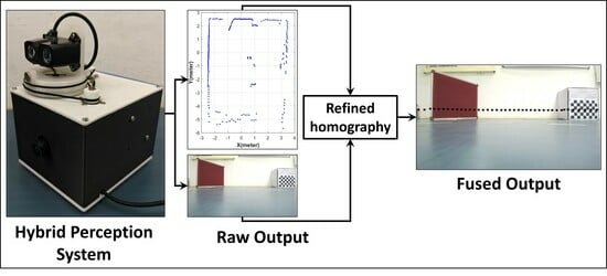
This section describes the development of an HPS, which consists of a rotating 2D LiDAR and a monocular camera. Subsequently, the developed calibration technique for fusing the data from both sensors is discussed. The overview of the developed calibration technique for the HPS is illustrated in Figure 1.

2.1. Hybrid Perception System (HPS)

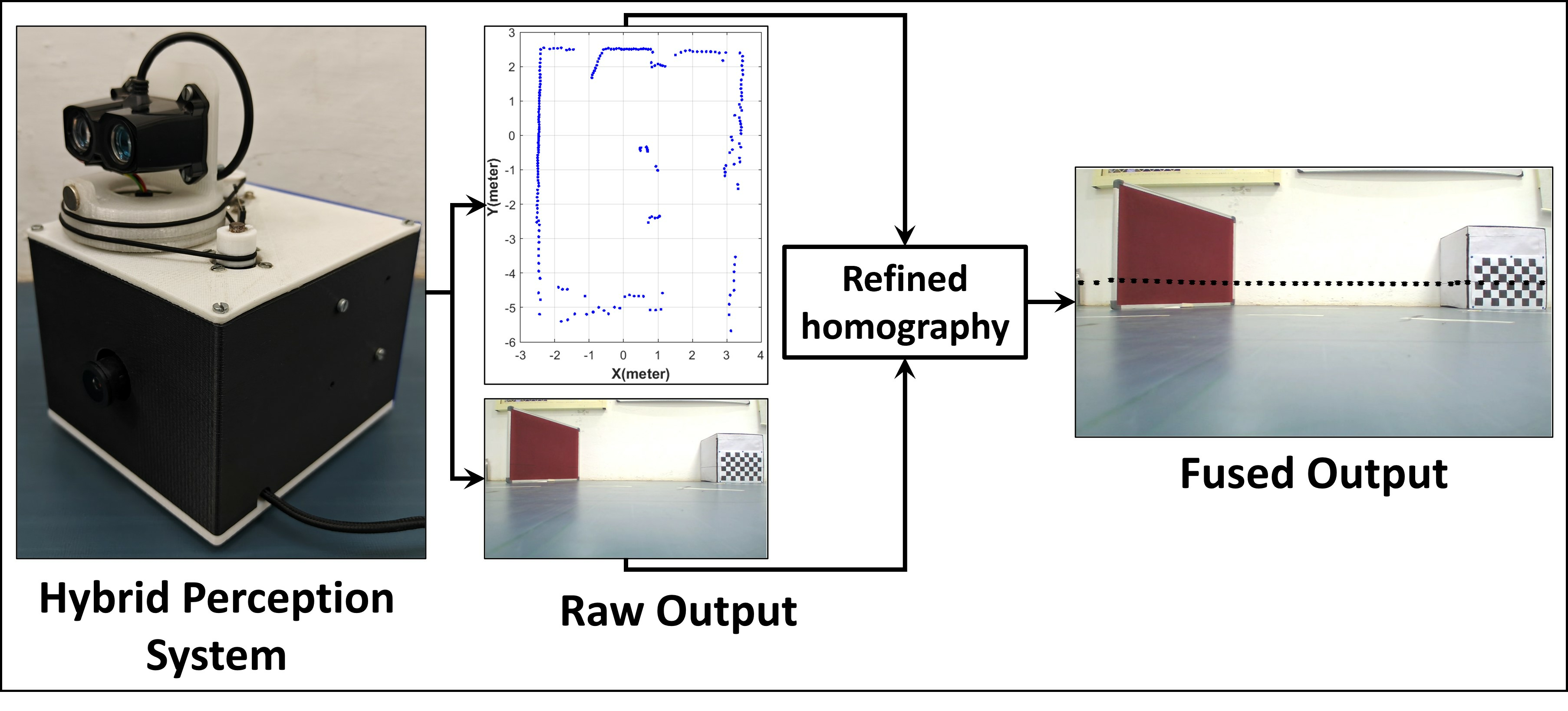
The developed HPS uses a Garmin 1D LiDAR (Model: LiDAR lite V3 HP—an IR LiDAR manufactured by Garmin, Olathe, KS, USA) and a 5MP USB monocular camera (IMX335 sourced from Evelta, Navi Mumbai, India). The selected LiDAR has an operating range of 40 m with a resolution of 1 cm and an accuracy of ± 2.5 cm. It should be noted that the operating voltage of the LiDAR is 5 V and the current consumption is 85 mA. This 1D LiDAR is converted into 2D LiDAR by providing continuous rotation using a DC motor, and the LiDAR rotation angle is obtained by attaching a rotary optical encoder to the motor shaft. An Arduino Mega 2560 microcontroller receives the LiDAR angular position ( θ ) from the feedback encoder (600 counts per revolution), and the distance ( d ) from the 1D LiDAR at each angular position and finds the 2D cartesian coordinates X L , Y L T . The HPS housing was designed and fabricated using the fused filament fabrication (FFF) process.
Figure 2 shows the construction of the HPS. A 438 RPM DC motor is used to provide continuous rotation to the LiDAR. The DC motor is driven by the L293D motor driver, which is powered by a 12 V power supply. The speed of the motor is controlled by the PWM signal from the Arduino Mega 2560 microcontroller. The LiDAR is fixed on the sensor housing with a pulley (as shown in Figure 2b), which is attached to the motor through a rubber belt (nitrile O-ring). Since the LiDAR rotates, it is connected to the microcontroller through the slip ring (used to make a connection between static and rotary parts). To obtain the angular position of the rotating sensor housing, an optical rotary encoder, which provides 600 counts per revolution, was used. An additional Hall sensor was used to track the completion of each revolution of the rotating LiDAR. The microcontroller reads the distance data from the LiDAR, the position counts from the encoder, and the Hall sensor output. Furthermore, the monocular camera of the HPS is interfaced with the PC to capture the streamed images and process them using the algorithm developed with the MATLAB R2022a software. This algorithm captures the camera image immediately after receiving the LiDAR scan from the microcontroller through serial communication on MATLAB. The camera resolution was set to 720 × 1280 pixels with other parameters such as brightness = 32, contrast = 25, and backlight compensation = 1.
Considering the sensor housing design parameters, such as the motor–sensor housing pulley ratio (1:5.75) and encoder–sensor housing pulley ratio (1:6), the angular position was computed as (6 × 600 = 3600 counts). If the angular position reaches 3600 counts, it is the completion of one LiDAR scan. However, since the sensor housing is an additively manufactured component, the error between design and fabrication persists. Hence, manually, it is estimated that the encoder–sensor housing pulley ratio is 1:5 with this, and the maximum angular position for a single LiDAR scan was set to 3000 counts. The 2D LiDAR scans (consecutive ten scans) obtained using this approach are shown in Figure 3a. From Figure 3a, it can be noticed that, even if the HPS is kept static, the LiDAR scans deviate or have an angular error over time due to setting the maximum angular position count by considering the encoder count and encoder–sensor housing pulley ratio. Moreover, with this problem, it is impossible to estimate the pose of the ego vehicle with LiDAR using any scan matching algorithm (i.e., even if the ego vehicle is static, the LiDAR scan will have angular deviation). To overcome this issue, a Hall sensor with a magnet was implemented to detect the closing angle of 0° or 360° for every LiDAR scan.
The procedure to obtain a closing angle with the Hall sensor is discussed below. Generally, the Hall sensor determines the output as “zero—if magnet detected” or “one—if magnet not detected” or vice-versa. In this work, the accurate closing angle was computed from the Hall sensor output. Figure 3b shows the output of the Hall sensor and the closing angle is exactly at the center of the magnet or zeros (i.e., Meanpeak). To find this Meanpeak, it is essential to find the one-to-zero (Endpeak) and zero-to-one (Startpeak) transition, which is depicted as a RED point and BLUE point, respectively, in Figure 3b. Now, the Meanpeak (GREEN point) is obtained for consecutive LiDAR scans and the encoder count is separated for each LiDAR scan. However, the encoder is an incremental encoder i.e., for the first scan, it counts from 0 to 3000, and for the second scan, the count value increases from 3001 to 6000, and so on. Hence, to obtain the absolute value of the encoder count for each scan, the first encoder count has to be detected (i.e., 0 and 3001) and then subtracted with all the encoder counts. Now, all the LiDAR scans have encoder count values between 0 and 3000. Subsequently, the encoder count can be converted into an angular position using Equation (1).
θ i = e n c o d e r c o u n t i e n d v a l u e 2 π
where e n d v a l u e is the last value of the e n c o d e r c o u n t for each LiDAR scan, θ i is the angular position that ranges between 0° and 360° or from 0 to 2π, and ‘ i ’ is the number of samples present in a single LiDAR scan. The angular deviation-corrected 2D LiDAR scan is shown in Figure 3c. The 2D Cartesian coordinates can be computed using Equation (2). One problem with this approach is that the angular resolution is not a fixed value (like an industrial LiDAR sensor), which leads to inconsistent or uncertain LiDAR points that demand the system to develop a newer calibration technique.
X L Y L Z L = d cos θ d sin θ 0
Moreover, it should be noted that the developed HPS is a cost-effective alternate perception system to the existing 2D LiDAR systems. The cost of the developed HPS prototype is approximately USD 290, whereas the cost of established 2D LiDAR systems, such as RP LiDAR A3 (USD 780), RP LiDAR S2E (USD 516), YD LiDAR G4 (USD 504), and YD LiDAR TG15 (USD 624), are comparatively higher than the developed HPS. Furthermore, it is worth noting that the LiDAR used in the HPS offers a 40 m range, whereas the above-mentioned existing sensors offer a maximum range of 30 m. Also, the existing 2D LiDARs cannot perceive spatial information, which is a built-in feature of the developed HPS. Hence, an additional camera needs to be integrated with the existing 2D LIDARs to achieve the same capability of HPS, thereby increasing the cost. The major limitation of the developed HPS is that the sampling frequency of the LiDAR used is 1 kHz, whereas the existing LiDARs have a minimum sampling frequency of 2 kHz. This lower sampling frequency of the HPS is due to the limited frequency at which the laser pulses are generated in the LiDAR lite V3 HP used in it. If the laser pulse width and its frequency are controlled externally, it is possible to improve the sampling frequency of HPS, which is a part of our future work.

2.2. Software Time Synchronization

Once the LiDAR points are obtained, the camera image has to be captured at that time instant. The present work utilized software time synchronization for capturing the LiDAR scans and camera image frames at the same time. Since both the 2D LiDAR and camera are connected to the PC with MATLAB, as shown in Figure 2, the multi-sensor data acquisition system acquires the camera images immediately after receiving the LiDAR points. The camera used in the present work acquires image frames at 30 Hz frequency (i.e., for every 33 milliseconds images can be captured), which is higher than that of LiDAR. The image that exactly represents the same scene point should be acquired within 33 milliseconds of the obtained 2D LiDAR scan. As mentioned in [24], the present work assumed that the time taken to capture one LiDAR scan is T L and for capturing camera images, it is T C . For ‘ m ’ LiDAR scans, the captured image frames are n T L T C . For time synchronization, the time difference between LiDAR and camera data ( i. e. ,   n T L T C m T L T C < 1 f ) should be less than 1 f , where ‘ f ’ is the frequency of the camera images (i.e., 30 Hz) and ‘ n ’ is the number of images. In the present work, from the multi-sensor data acquisition system, it is found that the average time taken for n T L T C m T L T C is 1.75 milliseconds, which is lower than 33 milliseconds. Hence, the captured LiDAR and camera data are well synchronized and represent the same scene point accurately in both sensor modalities.

2.3. Extraction of LiDAR–Camera Corresponding Points

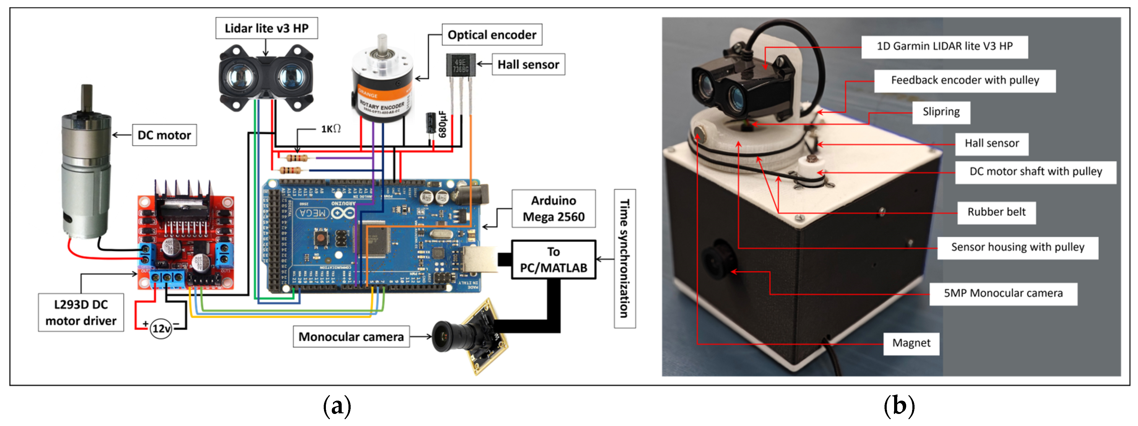
The LiDAR–camera calibration setup is shown in Figure 4. This work utilized a static pattern and a movable planar board to obtain the corresponding points between two sensors to estimate the homography matrix (i.e., a 3 × 3 matrix). Generally, estimating homography requires four or more corresponding points with no more than two collinear points [17]. To satisfy this condition, in this work, the edges of the calibration pattern, called edge points (five edges labeled as P 1 , P 2 , P 3 , P 4 , and P 5 ), were considered as the correspondence points. These edge points were marked as BLACK-colored dots, as shown in Figure 4, and from these dots, the feature points on the camera image could be obtained.
It can be said that this plane (RED/BLUE line from Figure 4) is the LiDAR plane, where Z L = 0 . However, to find these points on the 2D image, an IR camera was used to identify the LASER spots at the edges of the calibration pattern, as shown in Figure 5. However, finding the respective edge points in the LiDAR scan is difficult, since the LiDAR points may not be obtained at the edges due to their angular resolution.
For a given LiDAR point cloud, the edge points ( P 1 , P 2 , P 3 , P 4 , P 5 ) are extracted using a semi-automated approach, which is nothing but a separate edge point extraction algorithm coded in MATLAB. In this algorithm, initially, the Wall-1 and Wall-2 points (RED and GREEN triangle points shown in Figure 6 are selected using the MATLAB ‘ginput’ function. Generally, the ‘ginput’ function identifies the cursor movement and its click. Let us say that there are ten points present on a line segment AB. If the cursor is clicked at A and B, the number of points present between the AB line segments can be obtained. In the present case, as shown in Figure 6, the cursor is clicked twice (starting and ending point) on the Wall-1 LiDAR points (RED triangle), clicked twice on the Wall-2 (GREEN triangle), and clicked twice on the movable pattern (MAROON triangle) to extract the LiDAR points present between the two locations. Since the dimensions of the static and movable patterns are known (also the location of the static pattern), if the intersection of the Wall-1 and Wall-2 points is obtained, only with the movable pattern LiDAR points can the edge points’ location be computed automatically. To obtain the Wall-1 and Wall-2 intersection point, the slope along the x-axis and y-axis is considered as shown in Equation (3) and Equation (4), respectively. Using S l o p e y and S l o p e x , the Wall-1 and Wall-2 points can be separated and fitted with the least squares method. For Wall-1, the fitting equation is y = m 1 x + c 1 , and for Wall-2, it is y = m 2 x + c 2 . From the coefficients m 1 , m 2 , c 1 , a n d   c 2 , the Wall intersection points x wint ,   y wint can be obtained from Equation (5).
S l o p e y = x 2 x 1 y 2 y 1
S l o p e x = y 2 y 1 x 2 x 1
x wint ,   y wint = c 2 c 1 m 1 m 2 , m 1 x wint + c 1
Using the known location of the static pattern and Wall intersection point x wint ,   y wint , the edge point ( P 3 ) is computed as a point that is located at a known distance away from the Wall intersection point on the x-axis. Subsequently, with the known dimension of the static pattern, the edge points ( P 2 and P 1 ) are obtained. Furthermore, with the LiDAR points obtained on the movable pattern (MAROON triangle), the intersection (Equation (5)) of the Wall-2 and the movable pattern is the next edge point ( P 4 ). Finally, with the known dimension of the movable pattern, the edge point ( P 5 ) is obtained. Thus, a total of five edge points (corresponding points) are obtained. However, if we have more correspondence points, the HPS calibration accuracy will be better. Hence, to obtain more correspondence points between the detected edge points, a 1D interpolation was used. The 1D interpolation was conducted between ( P 1 P 2 , P 2 P 3 , P 3 P 4 , and P 4 P 5 ), and between each pair (let us say P 1 P 2 ), 25 equally spaced points were taken. Therefore, a total of 4 point pairs were available per LiDAR scan/camera image pair (i.e., 4 × 25 = 100). Hence, for each LiDAR scan/camera image pair, 100 corresponding points (interpolated) were considered. The corresponding points obtained from the image and LiDAR scan are shown in Figure 6 and Figure 7, respectively.

2.4. Standard Homography Estimation

Generally, any LiDAR point can be projected onto the camera image using a 3 × 3 homography matrix H , as shown in Equation (6). The standard homography matrix can be computed using the singular variable decomposition (SVD) or direct linear transform (DLT) method by solving the system of equations.
s u pred s v pred s = h 1 h 2 h 3 h 4 h 5 h 6 h 7 h 8 h 9 X L Y L Z L
The system of equations can be expressed as in Equation (7).
X L Y L 1 0 0 0 u X L u Y L u 0 0 0 X L Y L 1 v X L v Y L v h 1 h 2 h 3 h 4 h 5 h 6 h 7 h 8 h 9 = 0
The image pixel coordinates can be obtained using the following Equation (8).
u p r e d v p r e d = s u p r e d s s v p r e d s
where [ s u p r e d , s v p r e d ] T is the homogeneous representation of the actual 2D camera image point [ u , v ] T of a 3D scene point and [ X L , Y L ] T is its 2D LiDAR coordinate, and ‘ s 
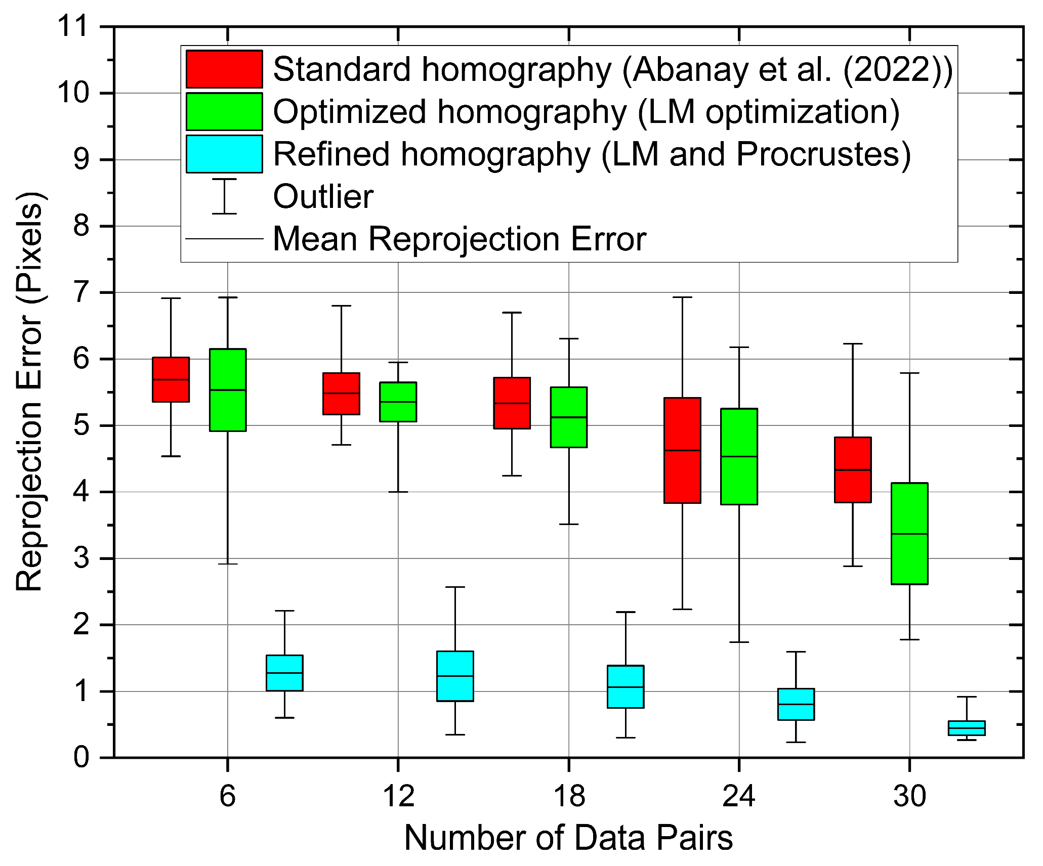
’ is the scale factor. The standard homography matrix is computed by establishing the system of equations with the corresponding points. However, reprojection using the standard homography matrix experiences a higher rotation error, which increases the reprojection error.

2.5. Optimized Homography Matrix

Hence, to minimize the rotation error, non-linear least squares optimization was performed using the Levenberg–Marquardt (LM) algorithm. LM optimization is an iterative method that finds the optimal homography matrix by minimizing the error ( E ( h ) ) between the real image points and projected LiDAR points onto the image. The homography matrix computed using SVD is introduced as the initial guess to the LM algorithm for quicker convergence.
The error function ( E ( h ) ) can be expressed as in Equation (9).
E ( h ) = u u p r e d v v p r e d
The optimized homography matrix can be obtained by minimizing the error function ( E ( h ) ) using the LM technique, as shown in Equation (10).
m i n h E ( h ) = m i n h i = 1 n E 2 ( h )
Now, with the optimized homography matrix, the rotation error is minimized. However, as the developed HPS has inconsistent LiDAR points due to the varying angular resolution, with the established corresponding points, the LM method optimizes the standard homography matrix with the local convergence or becomes trapped in the local minimum. In other words, the translation (distance) error is not minimized.

2.6. Refined Homography Using Procrustes Analysis

To minimize the translation error with the optimized homography matrix, a Procrustes analysis was performed. Procrustes analysis is a technique used to compare and align two sets of points or shapes to find an optimal transformation that minimizes the differences between them. Here, the actual 2D image points [ u , v ] T are compared to the [ u p r e d , v p r e d ] T obtained using an optimized homography matrix.
u f i n a l v f i n a l = b u p r e d v p r e d T 2 x 2 + c x c y
In Equation (11), [ u f i n a l , v f i n a l ] T is the near-accurate projected LiDAR point onto the image, and ‘ b ’ is the scale factor ( 1 b 1 ) . If b < 1 , the distance between the projected points is reduced, and, if b > 1 , the points are stretched; however, if b = 1 , the points are projected on the expected location of the image. [ T ] 2 x 2 is the transformation matrix; if det T = 1 , it is a reflection matrix, or if det T = 1 , [ T ] 2 x 2 is a rotation matrix. In 2D space, the reflection matrix can be expressed as c o s 2 θ s i n 2 θ s i n 2 θ c o s 2 θ and the rotation matrix can be expressed as c o s θ s i n θ s i n θ c o s θ . However, in both cases, ‘ θ ’ has to be computed, and it can be computed using Equation (12).
θ = t a n 1 i = 1 k ( u p r e d i · v v p r e d i · u ) i = 1 k ( u p r e d i · u + v p r e d i · v )
Furthermore, [ c x , c y ] T is the refined translation vector and it can be obtained as the mean of the predicted points (i.e., c x c y = i = 1 k u p r e d k i = 1 k v p r e d k ), and the scale factor ( b ) can be obtained as the root-mean-square distance (i.e., b = i = 1 k u p r e d i c x 2 + v p r e d i c y 2 k , where ‘ k ’ is the number of points). By substituting all the parameters in Equation (11), the refined reprojected LiDAR points onto the image can be computed. The next section discusses the performance of the proposed calibration approach through various experiments.

3. Experimental Results and Discussion

Experiments were conducted to verify the efficacy of the developed HPS and the calibration technique. This was verified by projecting the transformed LiDAR points obtained using the proposed calibration approach onto the camera image. The evaluation metrics considered in this paper were the mean reprojection error (MRE), rotation error, and translation error. Since the image points and corresponding LiDAR points are known, the MRE can be calculated by projecting the LiDAR points onto the image. Figure 8 shows the MRE obtained using various approaches: i.e., standard homography [17], optimized homography, and refined homography. A total of 30 data pairs of LiDAR scan and camera image were used for estimating the calibration parameters. The MRE obtained with the proposed method was 0.45 pixels, which is much lower than the MRE value reported in the literature. However, this MRE will vary depending on the distance between the HPS and the target. Hence, to study this MRE variation (qualitatively and quantitatively), additional experiments were conducted. Also, it can be seen that the reprojection error is reduced with the increase in number of data pairs for the refined homography method presented in this paper than the standard homography estimation. It may be noted that a further increase in the number of data pairs may reduce the reprojection error; however, it will not have a significant influence on the MRE. Hence, 30 data pairs are sufficient to achieve an MRE of less than 0.5 pixels.

3.1. Qualitative Comparison

A qualitative comparison was conducted by analyzing the reprojection error at varying distances and varying orientations. The experiments were conducted by keeping the evaluation pattern (white planar board as shown in Figure 9) at varying distances from the developed HPS and also at varying orientations (Figure 10). The LiDAR points were reprojected onto the image and are shown in Figure 9. It can be seen that, as the distance between HPS and the target increases, the number of LiDAR points decreases. Since the ground truth image points are unknown, the edge point on the evaluation pattern is obtained manually and the straight-line equation is computed (BLACK line). From Figure 9, it can be seen that, at a closer distance (1 m), the reprojected points using the standard homography possess a larger error. This is because distortions in the camera lens may become more significant at closer distances; hence, standard homography fails to compute an accurate calibration matrix. Furthermore, at closer distances, the accuracy of the LiDAR generally drops, which leads to a higher reprojection error. However, even at closer distances, the presented refined homography possesses a lower reprojection error due to the minimized rotation error using LM optimization and minimized translation error using Procrustes analysis. Moreover, from Figure 9c,d, it can be seen that the projected LiDAR points are slightly below the reference straight line (BLACK line), whereas, in Figure 9a,b,e, the projected LiDAR points are above the straight line. The possible reason for this is the influence of the surface irregularities on the computed calibration matrix. To verify this, we collected wheel odometry data ( x , y , z ) of the floor using the Pioneer P3DX mobile robot. Interestingly, it is found that the floor’s surface flatness varies in the range of ± 3.5 mm. If the HPS is placed on this irregular surface, it affects the LiDAR plane (i.e., Z L 0 ). This LiDAR plane error causes the calibration matrix to project the LiDAR points onto the camera image shifted downward to the reference line. Though it is shifted downward, the refined homography minimizes the projection error (however, still in the downward direction). Hence, it can be noticed that the developed refined homography approach delivers a highly accurate 2D LiDAR–camera fusion, irrespective of the distances.
Furthermore, the accuracy of the developed calibration technique was evaluated using the 2D LiDAR–Camera data acquired from the HPS placed at different orientations (in the present case, it was 60 ° , 90 ° , and 120 ° ). The LiDAR point cloud projected on the image frame is shown in Figure 10. It can be seen that, like the varying distance experiment, the varying orientation experiment with HPS results in a reduced reprojection error with the refined homography technique when compared to the standard and optimized homography techniques.
Subsequently, to further evaluate the robustness of the developed calibration approach, it was tested with a LiDAR scan/camera image pair obtained for special cases, i.e., the corner of the Wall, on an obstacle, and also with the calibration pattern itself. From the results illustrated in Figure 11, it can be seen that the proposed calibration approach accurately transforms the LiDAR points into image pixels with its improved calibration parameter estimation. Unlike Figure 9 and Figure 10, the results presented in Figure 11a,b show the effectiveness of the refined homography for varying depth conditions. Furthermore, Figure 11c illustrates the projection of LiDAR points onto the obstacle (battery car). If this obstacle is detected by any vision-based algorithm, using the projected LiDAR points, the obstacle’s distance can be estimated without the need of implementing LiDAR-based obstacle detection. In contrast to the existing methods, the current approach facilitates an accurate LiDAR to camera transformation, improving obstacle distance detection. This enhancement is particularly valuable for applications such as obstacle avoidance and emergency braking systems.
To explore the effectiveness, the accuracy of the proposed calibration method was also evaluated by transforming the image pixels into LiDAR coordinates using the computed calibration matrix. In other words, this experiment was conducted to validate the performance of the developed calibration technique for varying pose conditions. Figure 12 shows the reprojected image pixels onto the LiDAR scan using the developed calibration approaches for the test condition presented in Figure 11a,b. Furthermore, it can be observed that, as mentioned in Section 2.4, the rotation error is higher with the standard homography method (RED line). However, this rotation error is reduced with the optimized homography estimation (GREEN line), but this approach introduces a significant translation error. Finally, the refined homography matrix solves the translation error problem (shown as a CYAN line), which is close to the ground truth LiDAR points (BLACK line).

3.2. Quantitative Comparison

For the results presented in the previous section, a quantitative analysis was carried out using the proposed calibration approach and is discussed in this section. Like in the previous section, the analysis is divided into three parts: (a) with varying distances between the HPS sensor and target (Figure 9), (b) with varying orientations (Figure 10), and (c) with data obtained using the calibration pattern, and by scanning the Wall corner (Figure 12). For the first analysis, the distance error and rotation error were considered. The distance error was estimated as the normal distance between the image line and the projected point. Furthermore, the rotation error was estimated as the angle between the image line and the line obtained using reprojected points.
From Table 1, it can be seen that the rotation error and translation error are reduced by 68.0% and 36.4% with optimized homography and by 71.4%, and 71.8% with refined homography, respectively, when compared to the standard homography estimation technique. This minimization in the rotation and translation errors is mainly due to the use of the LM optimization technique in the optimized homography method. However, the translation error is not reduced as much as the rotational error. Hence, as mentioned in the previous section, the application of Procrustes analysis along with LM optimization (refined homography) provides a further reduction in the translation error. Furthermore, it is worth noting that, as the distance increases, the rotation error decreases for all the methods; however, optimized homography shows a vast improvement when compared to the standard homography. This is mainly due to the LM optimization that minimizes the error between the actual image coordinates and predicted image coordinates of the LiDAR point. On the other hand, the Procrustes analysis helps in reducing the translation error and it can be seen in the distance error between standard homography and refined homography. This is due to the refined translation vector [ c x , c y ] T obtained from the Procrustes analysis.
Additionally, the analysis of average error reveals a substantial improvement with the refined homography method, showing a 65.08% reduction in the rotation error and a 71.93% reduction in the distance error compared to the standard homography estimation. Furthermore, when compared to the optimized homography estimation, the refined homography method still demonstrates notable enhancements, with a 4.34% reduction in the rotation error and a substantial 58.18% reduction in the distance error. These results underscore the significant advantages of the refined homography method in reducing both rotation and distance errors compared to the standard homography estimation technique.
Furthermore, for the reprojected 2D LiDAR points presented in Figure 10, the rotational and distance errors are computed and tabulated in Table 2. From Table 2, it can be noticed that the refined homography shows the reduced error for varying orientations. When compared to the standard homography technique, the developed refined homography reduced the rotation error by 47.06% and distance error by 78.4%.
Subsequently, the quantitative analysis was extended for the reprojected image pixels onto the LiDAR scan, as shown in Figure 12. From Table 3, it can be noticed that the rotation error ( r x , r y ) obtained using optimized homography is (−0.38°, 0.55°), which amounts to a reduction of (94.4%, 89.7%), respectively, compared to the standard homography technique. The use of the refined homography method helped to further reduce the rotation error marginally by (95.5% and 91.4%), when compared to standard homography. On the other hand, the translation error ( t x , t y ) shows an error reduction of 12.6% and 24.1% with the optimized homography technique. However, with refined homography, we achieved a substantial reduction in the translation error (i.e., 97.1% and 90.0%) compared to the standard homography technique. The numbers clearly show that the developed calibration techniques (optimized and refined homography) outperform the standard homography-based extrinsic parameter estimation.

4. Conclusions

This paper presents the development of a new 2D LiDAR–camera calibration approach that utilizes the LM algorithm and Procrustes analysis for estimating the extrinsic parameters of a low-cost hybrid perception system (HPS)—which is under development. As a first step, the problem of angular deviation experienced by the 2D LiDAR, due to rotational variation, was addressed by implementing a Hall sensor. Furthermore, the homography matrix was estimated and optimized using the Levenberg–Marquardt (LM) algorithm that guarantees a minimized rotational error. Then, a Procrustes analysis was performed to minimize the distance error. From the experimental results, it can be seen that the developed refined homography approach shows significant improvement in terms of a reduction in MRE (0.45 pixels), rotation error ( r x , r y ) = (−0.31°, 0.46°), and distance error ( t x , t y ) = (2.82 mm, 11.44 mm) compared to the standard homography estimation technique. Moreover, this improved method accurately transforms the LiDAR point cloud data obtained from the environment, like Walls and obstacles. This improved performance of the developed HPS can help in developing safer autonomous navigation/obstacle avoidance algorithms and odometry estimation, which are the future directions of this research.

Author Contributions

Conceptualization, R.R. and P.V.M.; methodology, R.R. and P.V.M.; software, R.R.; validation, R.R. and P.V.M.; formal analysis, R.R. and P.V.M.; investigation, R.R. and P.V.M.; resources, R.R.; data curation, R.R.; writing—original draft preparation, R.R.; writing—review and editing, R.R. and P.V.M. All authors have read and agreed to the published version of the manuscript.

Funding

This work was supported in part by the Indian Institute of Technology Madras, funded by the Indian Government (PMRF scheme) under Grant SB22230168MEPMRF000758.

Institutional Review Board Statement

Not applicable.

Informed Consent Statement

Not applicable.

Data Availability Statement

The raw data supporting the conclusions of this article will be made available by the authors upon request.

Conflicts of Interest

The authors declare no conflicts of interest.

References

  1. Li, G.; Liu, Y.; Dong, L.; Cai, X.; Zhou, D. An algorithm for extrinsic parameters calibration of a camera and a laser range finder using line features. In Proceedings of the 2007 IEEE/RSJ International Conference on Intelligent Robots and Systems, San Diego, CA, USA, 29 October–2 November 2007; pp. 3854–3859. [Google Scholar] [CrossRef]
  2. Willis, A.R.; Zapata, M.J.; Conrad, J.M. A linear method for calibrating LIDAR-and-camera systems. In Proceedings of the IEEE Computer Society’s Annual International Symposium on Modeling, Analysis, and Simulation of Computer and Telecommunications Systems (MASCOTS), London, UK, 21–23 September 2009; pp. 577–579. [Google Scholar] [CrossRef]
  3. Meng, L.; Sun, F.; Ge, S.S. Extrinsic calibration of a camera with dual 2D laser range sensors for a mobile robot. In Proceedings of the 2010 IEEE International Symposium on Intelligent Control, Yokohama, Japan, 8–10 September 2010; pp. 813–817. [Google Scholar] [CrossRef]
  4. Kwak, K.; Huber, D.F.; Badino, H.; Kanade, T. Extrinsic calibration of a single line scanning LiDAR and a camera. In Proceedings of the 2011 IEEE/RSJ International Conference on Intelligent Robots and Systems, San Francisco, CA, USA, 25–30 September 2011; Institute of Electrical and Electronics Engineers (IEEE): Piscataway, NJ, USA, 2011; pp. 3283–3289. [Google Scholar] [CrossRef]
  5. Guo, C.X.; Roumeliotis, S.I. An Analytical Least-Squares Solution to the Line Scan LIDAR-Camera Extrinsic Calibration Problem. In Proceedings of the International Conference on Robotics and Automation (ICRA), 2013 IEEE International Conference, Karlsruhe, Germany, 6–10 May 2013; pp. 58–63. [Google Scholar]
  6. Zhou, L. A new minimal solution for the extrinsic calibration of a 2D LIDAR and a camera using three plane-line correspondences. IEEE Sens. J. 2014, 14, 442–454. [Google Scholar] [CrossRef]
  7. Zhou, L.; Deng, Z. A new algorithm for the extrinsic calibration of a 2D LIDAR and a camera. Meas. Sci. Technol. 2014, 25, 065107. [Google Scholar] [CrossRef]
  8. Ahmad Yousef, K.M.; Mohd, B.J.; Al-Widyan, K.; Hayajneh, T. Extrinsic calibration of camera and 2D laser sensors without overlap. Sensors 2017, 17, 2346. [Google Scholar] [CrossRef] [PubMed]
  9. Dong, W.; Isler, V. A Novel Method for the Extrinsic Calibration of a 2D Laser Rangefinder and a Camera. IEEE Sens. J. 2018, 18, 4200–4211. [Google Scholar] [CrossRef]
  10. Itami, F.; Yamazaki, T. A simple calibration procedure for a 2D LiDAR with respect to a camera. IEEE Sens. J. 2019, 19, 7553–7564. [Google Scholar] [CrossRef]
  11. Ye, Q.; Shu, L.; Zhang, W. Extrinsic Calibration of a Monocular Camera and a Single Line Scanning LiDAR. In Proceedings of the 2019 IEEE International Conference on Mechatronics and Automation, Tianjin, China, 4–7 August 2019; pp. 1047–1054. [Google Scholar]
  12. Chu, X.; Zhou, J.; Chen, L.; Xu, X. An Improved Method for Calibration between a 2D LiDAR and a Camera Based on Point-Line Correspondences. In Proceedings of the 2019 3rd International Conference on Artificial Intelligence, Automation and Control Technologies (AIACT 2019), Xi’an, China, 25–27 April 2019; Journal of Physics: Conference Series; Institute of Physics Publishing: Bristol, UK, 2019; Volume 1267. [Google Scholar] [CrossRef]
  13. Palmer, A.H.; Peterson, C.; Blankenburg, J.; Feil-Seifer, D.; Nicolescu, M. Simple Camera-to-2D-LiDAR Calibration Method for General Use. In Proceedings of the Advances in Visual Computing: 15th International Symposium, San Diego, CA, USA, 5–7 October 2020; pp. 193–206. [Google Scholar]
  14. Kim, J.Y.; Ha, J.E. Extrinsic calibration of a camera and a 2D LiDAR using a dummy camera with IR cut filter removed. IEEE Access 2020, 8, 183071–183079. [Google Scholar] [CrossRef]
  15. Itami, F.; Yamazaki, T. An Improved Method for the Calibration of a 2-D LiDAR with Respect to a Camera by Using a Checkerboard Target. IEEE Sens. J. 2020, 20, 7906–7917. [Google Scholar] [CrossRef]
  16. Liu, C.; Huang, Y.; Rong, Y.; Li, G.; Meng, J.; Xie, Y.; Zhang, X. A Novel Extrinsic Calibration Method of Mobile Manipulator Camera and 2D-LiDAR Via Arbitrary Trihedron-based Reconstruction. IEEE Sens. J. 2021, 21, 24672–24682. [Google Scholar] [CrossRef]
  17. Abanay, A.; Masmoudi, L.; El Ansari, M. A calibration method of 2D LIDAR-Visual sensors embedded on an agricultural robot. Optik 2022, 249, 168254. [Google Scholar] [CrossRef]
  18. Manouchehri, M.; Ahmadabadian, A.H. Extrinsic calibration of a camera and a 2D laser range finder using ping pong balls and the corner of a room. Measurement 2023, 216, 113011. [Google Scholar] [CrossRef]
  19. Beltrán, J.; Guindel, C.; de la Escalera, A.; García, F. Automatic Extrinsic Calibration Method for LiDAR and Camera Sensor Setups. IEEE Trans. Intell. Transp. Syst. 2022, 23, 17677–17689. [Google Scholar] [CrossRef]
  20. Sun, Y.; Li, J.; Wang, Y.; Xu, X.; Yang, X.; Sun, Z. ATOP: An Attention-to-Optimization Approach for Automatic LiDAR-Camera Calibration via Cross-Modal Object Matching. IEEE Trans. Intell. Veh. 2023, 8, 696–708. [Google Scholar] [CrossRef]
  21. Koide, K.; Oishi, S.; Yokozuka, M.; Banno, A. General, Single-shot, Target-less, and Automatic LiDAR-Camera Extrinsic Calibration Toolbox. arXiv 2023, arXiv:2302.05094. [Google Scholar]
  22. Zhang, B.; Zheng, Y.; Zhang, Z.; He, Q. LiDAR and Camera Calibration Using Pyramid and Checkerboard Calibrators. In Proceedings of the 2023 IEEE 8th International Conference on Big Data Analytics, ICBDA 2023, Harbin, China, 3–5 March 2023; Institute of Electrical and Electronics Engineers Inc.: Piscataway, NJ, USA, 2023; pp. 187–192. [Google Scholar] [CrossRef]
  23. Fan, S.; Yu, Y.; Xu, M.; Zhao, L. High-Precision External Parameter Calibration Method for Camera and LiDAR Based on a Calibration Device. IEEE Access 2023, 11, 18750–18760. [Google Scholar] [CrossRef]
  24. Wang, C.; Liu, S.; Wang, X.; Lan, X. Time Synchronization and Space Registration of Roadside LiDAR and Camera. Electronics 2023, 12, 537. [Google Scholar] [CrossRef]
Figure 1. Overview of the developed calibration technique for the hybrid perception system.
Vehicles 06 00033 g001
Figure 2. Developed hybrid perception system: (a) HPS circuit connection and (b) assembly with HPS housing.
Vehicles 06 00033 g002
Figure 3. Two-dimensional LiDAR scan obtained from the developed HPS. (a) Two-dimensional LiDAR scan with angular deviation; (b) estimated closing angle using Hall sensor output, and (c) corrected 2D LiDAR scan without angular deviation.
Vehicles 06 00033 g003
Figure 4. Two-dimensional LiDAR–camera calibration setup. RED points represent 2D LiDAR points. BLACK points represent the manually obtained corresponding image pixels. BLUE lines represent 2D LiDAR planes.
Vehicles 06 00033 g004
Figure 5. Laser spot on one of the edges of the calibration pattern.
Vehicles 06 00033 g005
Figure 6. Edge points and interpolated points on the LiDAR scan.
Vehicles 06 00033 g006
Figure 7. Edge points and interpolated points on the image. Due to the limited field of view of the camera, Wall-1 is not visible, and Wall-2, static pattern, movable pattern, and floor are depicted.
Vehicles 06 00033 g007
Figure 8. Comparison of the reprojection error. Standard homography [17] by Abanay et al. (2022).
Vehicles 06 00033 g008
Figure 9. Reprojected 2D LiDAR points onto the image at different distances: (a) 1 m, (b) 2 m, (c) 3 m, (d) 4 m, and (e) 5 m. RED points indicate reprojection using standard homography, and GREEN points indicate reprojection using optimized homography. CYAN points indicate reprojection using refined homography, and the black line indicates ground truth.
Vehicles 06 00033 g009
Figure 10. Reprojected 2D LiDAR points onto the image at different orientations: (a) 60 degrees, (b) 90 degrees, and (c) 120 degrees. RED points indicate reprojection using standard homography, and GREEN points indicate reprojection using optimized homography. CYAN points indicate reprojection using refined homography, and the black line indicates ground truth.
Vehicles 06 00033 g010
Figure 11. Reprojected LiDAR points onto the image (a) on the calibration pattern, (b) on a Wall corner, and (c) on an obstacle. CYAN points indicate reprojection using the refined homography technique.
Vehicles 06 00033 g011
Figure 12. Reprojected image pixels onto the LiDAR scan (a) on the calibration pattern and (b) on a Wall corner.
Vehicles 06 00033 g012
Table 1. Comparison of the rotational error and distance error at varying distances.
Distance (m)Standard Homography [17]Optimized HomographyRefined Homography
Rotation Error (deg)Distance Error (Pixel)Rotation Error (deg)Distance Error (Pixel)Rotation Error (deg)Distance Error (Pixel)
11.177.600.644.550.621.87
20.588.060.175.690.151.95
30.323.310.071.460.051.08
40.4411.290.118.390.103.54
50.6212.490.188.610.163.55
Average0.638.550.235.740.222.40
Table 2. Comparison of the rotational error and distance error at varying orientations.
Orientation (deg)Standard Homography [17]Optimized HomographyRefined Homography
Rotation Error (deg)Distance Error (Pixel)Rotation Error (deg)Distance Error (Pixel)Rotation Error (deg)Distance Error (Pixel)
600.1816.300.116.160.093.52
900.1613.040.107.140.083.01
1200.1715.410.127.060.103.10
Average0.1714.920.116.790.093.21
Table 3. Comparison of the rotational error and distance error from the reprojected image pixels.
MethodRotation Error (deg)Absolute Mean Translation Error (mm)
r x r y t x t y
Standard Homography [17] by Abanay et al. (2022)−6.735.2997.66114.36
Optimized Homography−0.380.5585.3286.82
Refinement of Optimized Homography−0.310.462.8211.44
Disclaimer/Publisher’s Note: The statements, opinions and data contained in all publications are solely those of the individual author(s) and contributor(s) and not of MDPI and/or the editor(s). MDPI and/or the editor(s) disclaim responsibility for any injury to people or property resulting from any ideas, methods, instructions or products referred to in the content.

