A Novel Application of Fractional Order Derivative Moth Flame Optimization Algorithm for Solving the Problem of Optimal Coordination of Directional Overcurrent Relays

Abstract

The proper coordination of directional overcurrent relays (DOCRs) is crucial in electrical power systems. The coordination of DOCRs in a multi-loop power system is expressed as an optimization problem. The aim of this study focuses on improving the protection system’s performance by minimizing the total operating time of DOCRs via effective coordination with main and backup DOCRs while keeping the coordination constraints within allowable limits. The coordination problem of DOCRs is solved by developing a new application strategy called Fractional Order Derivative Moth Flame Optimizer (FODMFO). This approach involves incorporating the ideas of fractional calculus (FC) into the mathematical model of the conventional moth flame algorithm to improve the characteristics of the optimizer. The FODMFO approach is then tested on the coordination problem of DOCRs in standard power systems, specifically the IEEE 3, 8, and 15 bus systems as well as in 11 benchmark functions including uni- and multimodal functions. The results obtained from the proposed method, as well as its comparison with other recently developed algorithms, demonstrate that the combination of FOD and MFO improves the overall efficiency of the optimizer by utilizing the individual strengths of these tools and identifying the globally optimal solution and minimize the total operating time of DOCRs up to an optimal value. The reliability, strength, and dependability of FODMFO are supported by a thorough statistics study using the box-plot, histograms, empirical cumulative distribution function demonstrations, and the minimal fitness evolution seen in each distinct simulation. Based on these data, it is evident that FODMFO outperforms other modern nature-inspired and conventional algorithms.

1. Introduction

1.1. Inspiration and Motivation

The protection plan is an important requirement for the reliable operation of a power system. An effective protection plan promptly resolves a defect to provide uninterrupted power supply to the unaffected components of the system. Each component in an electrical power network is protected by two kinds of protections, namely main and backup protection. In order to provide a strong and reliable setup of an electrical power network, it is crucial that the main protection system for any faults reacts with utmost speed to separate the problematic section from the rest of the system. If the main network protection fails to clear the problem, its backup protection shall assume the duty of eliminating the fault. This is an ideal scenario for any protective plan, since the main defense only focuses on the impacted region. In contrast, when the secondary reinforcement is activated, a larger percentage of the system experiences unnecessary power interruptions. To ensure that only the specific area of the system that is impacted remains isolated while minimizing the possibility of unwanted power outages, it is necessary to have a dependable and efficient operation of the safety equipment. To ensure the efficiency and profitability of a multi-loop electrical power network, it is essential to use directional overcurrent relays (DOCRs) as part of the protection plan. The functioning and setup of directional overcurrent relays (DOCRs) are governed by two constraints: the time dial setting (TDS) and the plug setting (PS). The TDS and PS have a significant impact on the optimization of DOCRs, as they play a crucial role in determining the operational features and coordination of the DOCRs. The time delay of the DOCRs’ response is adjusted by the TDS in order to control the speed of fault clearance and selectivity. A lower TDS value results in a faster DOCRs response and action, which results in the ability to isolate the faults as rapidly as possible but may potentially lead to an unwanted operation in transient circumstances. On the other hand, a higher TDS value improves the selectivity but at the cost of delayed fault clearance, which may lead to damage by prolonged faults. Conversely, the PS determines the current threshold that triggers the DOCRs’ operation. It plays a key role in establishing how the DOCRs react to a fault event. Furthermore, the sensitivity of DOCRs is increased when the PS is lower, which enables the DOCRs to operate on low-magnitude faults, hence providing a more efficient protection for the system. However, this may lead to other non-fault situations or unwanted trips on load inrushes. In order to ensure the reliability and safety of the power system, the setting for TDS and PS should be precisely calculated to achieve an optimal balance between the sensitivity and selectivity of the DOCRs. The DOCRs effectively coordinate to manage the TDS and PS, ensuring that the main protection immediately and consistently eliminates the fault to the highest extent feasible. Furthermore, it is crucial to effectively coordinate the configuration of any DOCRs with other electrical equipment in order to prevent damage to the surrounding devices. Due to this design, the coordination issue may become slightly more complex.

1.2. Literature Review

In order to elucidate this complex matter, many different kinds of methodologies were developed according to the existing body of literature. The coordination issue of overcurrent relays was addressed in [1] using the linear approach. The configuration of relays in [2] was selected via graphical sequential programming. In [3], an expert method was used that exploits the minimum break point established. Additional methodologies include curve intersection [4] and graphical selection method [5].

Different versions of nature-inspired optimization, such as JAYA and whale optimization, were used by the authors of [6,7,8,9] in order to address the DOCR coordination issue that was present inside the electrical power network. The DOCR design created in [10,11] was the most optimal one in terms of the physical and logical changes that were made to the layout of the system. A hybrid genetic algorithm for DOCR coordination was employed in [12,13] in order to determine the optimal TDS and PS values of DOCRs while taking into consideration the possibility of a line or generator unit outage. The DOCR issue that occurred in a multi-loop transmission system as a result of single-line outage contingency has been addressed in [14,15]. The issue of protection coordination is very important in the design of DOCRs, which may sometimes function incorrectly as a result of changes in the configuration of the network. Instead of taking into account the possibility of line or DG failures, the fault current limiters were used in [16] in order to tackle the protection coordination issue. In [17], a new set of coordination parameters that correspond to line, substation, and DG failures was developed in order to overcome the issue of protection coordination for micro-grids. Additionally, the layout of all of these networks makes it more complicated, which results in the disorganization of DOCRs, which in turn persistently leads to unforeseen circumstances. In order to alleviate these concerns as well as the power outages, it has been advised in [18,19,20,21] that the ideal relay setting be used while taking into consideration the design of the primary system. The DOCR issue was stated as mixed integer nonlinear programming (MINLP), and it was addressed by using a variety of population-based optimization techniques, as described in [22,23]. In the papers [24,25], a linear formulation was designed in order to address the DOCR coordination problem. This was accomplished by developing a few bio-motivated algorithms. An alternative implementation of particle swarm optimization (PSO) was used in the research presented in [26,27,28,29,30] in order to ascertain the optimal values for DOCRs. In order to demonstrate the superiority of modified differential evolution algorithms, a revised version of the differential algorithm was reported in [31] in order to address the DOCR coordination issue. For the purpose of DOCR coordination, a great number of other nature-inspired algorithms, such as the modified electromagnetic field optimization (MEFO), improved firefly (IFA), mixed integer linear programming, grey wolf optimizer (GWO), biology-based optimization (BBO), teaching learning–based optimization (TLBO), and back-tracking algorithm were utilized in [32,33,34,35,36,37,38]. The article [39] used a modified version of the teaching-based optimization technique. There was an attempt made in [40] to solve the DOCR issue by using an analytical technique. A group search that was improved was used in the relay coordination process in [41]. In [42], a different version of the firefly algorithm was utilized to solve the DOCRs for various IEEE benchmark systems. Recent research has shown that integrating fractional calculus (FC) and the core concepts of fractional derivatives into the mathematical model of a system will provide significantly improved results in many scientific and engineering domains. A diverse array of issues, such as feature selection, image processing, hyperspectral visuals, controllers for forecasting robotic routes, Kalman filters, and fractional order filters, have been effectively addressed using these techniques. Based on this research, it is recommended to use FC approaches in conjunction with evolutionary strategies to tackle optimization challenges in the energy industry. Fractional-order robotic particle swarm optimization (FPSO) with a fraction order velocity has been extensively studied in various domains [43,44,45,46,47]. Otsu Image Segmentation was solved using with fractional order Moth flame optimizer [48]. In [49], fractional-order Darwinian particle swarm optimization is adapted for Kalman filtering computations. Additional uses include the creation of a multiband power system stabilizer that utilizes a lead–lag compensator using a hybrid dynamic GA-PSO [50], as well as the detection of non-linear systems [51] and fractional-order swarming optimizers for economic load dispatch [52], hybrid fractional computing with a gravitational search algorithm for DOCRs [53], and reactive power minimization with fact devices, which has been solved using a fractional evolutionary strategy [54]. The results of this study provide support for the use of FC tools in combination with metaheuristic algorithms for addressing optimization difficulties in the energy and power industry. The performance of the fractional-order metaheuristics methods is significantly influenced by the configurations of its parameters, including fractional-order settings, inertial weights, and accelerating coefficients. Early convergence, a lack of progress, or fluctuating behavior may be the consequence of inadequate parameter values, which would need careful correction and optimization. In the context of electrical power systems, the DOCR problem in a multisource network may be seen as an optimization problem. The disadvantage of the previous optimization processes and the metaheuristic optimization is that they have the potential to combine standards that may not be ideal in every situation, but are rather limited to a local optimal value. This is a drawback of both of these optimization methods. In this inquiry, a FODMFO algorithm approach is investigated in order to determine the precise and optimal DOCR coordination in comparison to other cutting-edge algorithms.

1.3. Contribution and Paper Structure

In electrical power systems, the accurate coordination of DOCRs involve careful selection for appropriate settings including TDS, Ip, and PS to ensure that a primary protection strategy is fulfilled while meeting the criteria of selectivity reliability, sensitivity, and speed. The estimated settings may not be optimal for all possible scenarios owing to the ambiguities associated with load variations, such as unexpected events or exceeding the desired current value, as well as variations in the system’s topology, including radial, parallel, ring, and connected topologies. Conventional computational methods are ineffective in finding a solution that is global and often become stuck in local optimal states due to the existence of several optimum points, continuous TDS and Ip variables, nonconvex features, and the inclusion of equations that are not linear in the coordination time. This research study presents a novel optimization approach known as FODMFO. This method improves the optimization capabilities of the traditional MFO algorithm, including its ability to convergence rate, by incorporating the principles of FC into its mathematical framework. This method is evaluated by identifying the minimum optimum total operating time for DOCRs’ coordination time. Minimizing the total operating time of DOCRs allows for a faster identification and isolation of faults, resulting in a considerable decrease in system downtime and an enhancement of overall operational efficiency. The implementation of this operational enhancement is crucial for ensuring the stability and uninterrupted functioning of systems, especially in intricate power distribution networks. This is achieved by adjusting the control settings, such as the TDS and PS. To evaluate the efficiency of the proposed FODMFO, three distinct case studies of an IEEE standard system are considered for the MINLP model.

The key and novel features of this research are as follows:

•

The mathematical model of MFO may be enhanced by including the concept of FC and FD integration. This integration aims to improve the optimization feature of MFO, namely its convergence rate.

•

To validate the performance of the proposed FODMFO, a total of 11 benchmark functions including unimodal and multimodal function have been solved in terms of mean fitness value among 100 independent runs.

•

The novel application of a fractional memetic computing approach, FODMFO, is used to minimize and optimize the operating time of DOCRs in a standard test system, by adjusting the values of TDS and PS.

•

The suggested scheme of a FODMFO aims to decrease the overall running duration of DOCRs in conventional networks. This is recognized by restricting the TDS and PS within acceptable ranges, considering varied topological and operational conditions.

•

The statistical illustrations, such as cumulative distribution function plots, box-plots, histogram illustrations, standard normal quantile plots, and minimum fitness value plots, are developed to assess the stability, accuracy, and robustness of the proposed FODMFO algorithm in independent runs.

2. DOCR Problem Formulation

The primary goal of DOCR coordination is to promptly detect faults and isolate the affected regions. In order to accomplish this objective in relay coordination, it is necessary to determine the optimal values for the TDS and PS of each DOCR. The goal is to reduce the overall time of operation of all principal DOCRs by meeting the particular constraints outlined in the objective function:

$$minf=\sum _{i=1}^n{T}_{i,j},$$

(1)

The variable T_i,j represents the duration of operation of the main relay in response to a fault occurring in zone j. Thus, the unique curvature used for the functioning of the relay Ri is picked from a specific subset of the decisions made in accordance with the International Electro Technical Commission IEC standard, in the following manner:

$$T_{op}=TD{S}_i\left[\frac{\alpha }{{\left(\frac{I{F}_i}{PS\times CTR}\right)}^k-1}\right]$$

(2)

$T_{op}$TDS, IF, PS, and CTR represent the total operating time, time dial setting, fault current, plug setting, and current transfer ratio (CTR), correspondingly, for standard inverted type relays. The values of the constants α and k are 0.14 and 0.02, respectively. Figure 1 displays the schematic diagram illustrating the coordination of DOCRs in an electrical power network.

2.1. Coordination Criterion

The coordination time interval (CTI) is used to provide synchronous coordination between the main and backup safety patterns in an electrical protection system. The CTI value may range from 0.2 to 0.5 s, depending upon several occurrences and causes. This section may be expressed as follows:

$${ T}_b\ge T_p+CTI,$$

(3)

where

• $T_p:$ the primary (or main) relay operating time;
• $T_b:$ the backup relay operating time.

2.2. Relay Setting Bounds

The total duration of the relays may be reduced by adhering to two essential factors: the constraints imposed by relay constraints and the limits of coordination. The major criteria establish the boundaries of TDS and PS, whilst other mandates pertain to the coordination of primary and backup relays. The allowable values for relay configuration parameters are determined by the constraints and design of the relay. These values may be described using the following ranges:

$${{TDS}_i}^{min}\le {TDS}_i\le {{TDS}_i}^{max}$$

(4)

$${{PTS}_i}^{min}\le {PTS}_i\le {{PTS}_i}^{max}$$

(5)

3. Design Methodology

A global search strategy that relies on the MFO algorithm and incorporates the idea of fractional calculus inside the mathematical framework of a classic MFO is used to address the constrained optimization issue. To assess the effectiveness and performance of the modified method, three case studies are conducted using IEEE 3, 8, and 15 bus systems. Figure 2 illustrates the suggested work technique.

3.1. Moth Flame Optimization (MFO)

The MFO algorithm is a metaheuristic optimization methodology inspired by the migratory patterns of moths in relation to moonlight. The moth utilizes a process known as transverse orientation to facilitate its locomotion. The possible solutions in the MFO algorithm are represented as moths. The optimization problem’s variables consist of the spatial location of the moths. The MFO is an algorithm that operates on a population of moths. The mathematical representation of the moths is as follows [55]:

$$M|=\left[\begin{array}{cc}\begin{array}{ccc}{M}_{\mathrm{1,1}}& M_{\mathrm{1,2}}& \dots ..\\ M_{\mathrm{2,1}}& M_{\mathrm{2,2}}& \dots ..\\ \begin{array}{c}\dots ..\\ M_{m,1}\end{array}& \begin{array}{c}\dots \dots \\ M_{m,2}\end{array}& \begin{array}{c}\dots \dots \\ \dots ..\end{array}\end{array}& \begin{array}{cc}\dots .& M_{1,n}\\ \dots .& M_{2,n}\\ \begin{array}{c}\dots \dots \\ \dots ..\end{array}& \begin{array}{c}\dots \dots \\ M_{m,n}\end{array}\end{array}\end{array}\right]$$

(6)

where n represents the number of variables and m represents the number of moths. The matrix for storing moths related to objective function values may be represented as follows:

$$\begin{array}{c}OM=\left[\begin{array}{c}{OM}_1\\ {OM}_2\\ \begin{array}{c}\dots .\\ {OM}_m\end{array}\end{array}\right]\end{array}$$

(7)

where m is the number of moths. Within the MFO algorithm, there are additional elements referred to as Flames. MFO initializes the population as follows:

$$M_{ij}=l{b}_i+u_j(u{b}_i-l{b}_i)$$

(8)

where ub_i and lb_i is the upper and lower bounds of ith variables.

The collection of flames is shown in the following manner:

$$\begin{array}{c}F=\left[\begin{array}{ccccc}{f}_{\mathrm{1,1}}& f_{\mathrm{1,2}}& \dots & \dots & f_{1,h}\\ f_{\mathrm{2,1}}& f_{\mathrm{2,2}}& \dots & \dots .& f_{2,h}\\ \dots & \dots & \dots & \dots & \dots \\ f_{m,1}& f_{m,2}& \dots .& \dots .& f_{m,h}\end{array}\right]\end{array}$$

(9)

The flames are arranged based on the values of the following objective function:

$$\begin{array}{c}OF=\left[\begin{array}{c}O{F}_1\\ O{F}_2\\ \dots \\ O{F}_m\end{array}\right]\end{array}$$

(10)

Both flames and moths are considered as solutions in the MFO algorithm. The primary distinction between flames and moths lies in the manner in which they are updated throughout each repetition. The moths traverse the search space. Flames may be seen as flags, and each moth explores the area surrounding a flag, updating it if a better solution is found. The mathematical model for tracking the movement of a moth in relation to a flame may be described as follows:

$$N=S\left(K_r-Y_w\right)$$

(11)

$$D_r=\left|Y_w-K_r\right|$$

(12)

$$S(K_r,Y_w)=D_r\cdot e^{qg}\cdot \mathrm{c}\mathrm{o}\mathrm{s} \left(2\pi g\right)+Y_w$$

(13)

$$D_r=\left\{\begin{array}{c}\left|F_i-M_i\right|, i\le f_{no}\\ F_{f_{no}}-M_i|, i>f_{no}\end{array}\right\}$$

(14)

where Y_w represents the wth flame, K_r represents the rth moth, and D_r represents the distance of the rth moth from the wth flame. The parameter q is a fixed value, whereas g is a randomly generated integer in the range of −1 to 1. The calculation for g may be performed in the following manner:

$$a=-1+Iter\times \left(\frac{-1}{Max.Iter}\right)$$

(15)

$$g=(a-1)\times rand+1$$

(16)

$$f_{no}=round(n-\frac{l}{L}(n-1))$$

(17)

At each location, Max.Iter represents the maximum number of iterations, whereas Iter represents the current iteration. Rand refers to a random integer between 0 and 1.

The MFO algorithm typically employs three functions, which may be stated as follows:

$$\begin{array}{c}MFO=(I,P,T)\end{array}$$

(18)

The function I generates a random population within the specified boundaries of the variables for the moths. It then calculates the fitness function values for each individual in the population. The function P is the primary function that is performed repeatedly until the function T evaluates as true. If the conversion conditions are not fulfilled, the function T evaluates as false. Otherwise, it evaluates as true and returns the search agents as the best achieved.

3.2. Fractional-Order Derivative Moth Flame Optimization (FODMFO)

The suggested approach combines fractional calculus (FC) with the basic MFO to create a fractional-order MFO algorithm. This integration aims to address the issue of accelerated convergence and provide satisfactory outcomes. The MFO algorithm has a favorable inclination toward global search, but its ineffective local search leads to a below-average decrease in convergence time. In order to overcome the constraint described earlier, the suggested technique incorporates FC into the core MFO approach. This integration allows for the use of the FC retention feature seen in previous solutions, ensuring the sharing of information across solutions throughout the exploitation phase. As a result, both the precision of the outcome and the pace at which it converges are changed. FC is particularly suitable for explaining complex events, such as irreversibility and chaos, due to the characteristics it uncovers and its intrinsic memory component. According to this theory, the constantly changing path of an MFO generates a distinct circumstance, where FC instruments are a good addition.

The application of FC in several scientific areas, including engineering, computer mathematics, and computational physics, has attracted the attention of many academics. FC is a mathematical framework that extends the concepts of integer-order calculus, addressing limitations that the latter could not overcome. Fractional derivatives, as an extension of integer derivatives, provide an appropriate approach for characterizing the memory and inherited characteristics of processes.

Multiple different methodologies exist for illustrating the concept of fractional-order derivatives [56,57]. The Grünwald–Letnikov theory may be used to deduce the FC-based mathematical equations for MFO by using fractional-order derivatives. Let us examine an arbitrary signal s(t) for which the Grünwald–Letnikov fractional-order derivative is expressed in the following equation:

$$D^{\delta }(s\left(t\right)=\underset{h\to 0}{\lim } \left[\sum _{k=0}^{\infty }\frac{{\left(-1\right)}^k\tau \left(\delta +1\right)s(t-kh)}{\tau (\delta -k+1)\tau (k+1)}\right]$$

(19)

While an integer-order derivative involves a limited series, a fractional-order derivative requires an unlimited number of terms. Derivatives of integers are thus considered to be “local” operators. Conversely, fractional derivatives possess an intrinsic ability to retain information about all previous occurrences. However, the impact of previous occurrences decreases as time passes. The discrete time computation is derived from the equation presented in Equation (17).

$$D^{\delta }(s\left(t\right)=\frac{1}{T^{\delta }} \left[\sum _{k=0}^{\infty }\frac{{\left(-1\right)}^k\tau \left(\delta +1\right)s(t-kh)}{\tau (\delta -k+1)\tau (k+1)}\right]$$

(20)

where the variable “T” represents the sample time, whereas “r” denotes the order of truncation. The variable “[s(t)]” is discrete, and in a specific scenario when δ equals one, the equation is converted to an integer order or ordinary first-order derivative and may be represented as follows:

$$D^1\left[s\left(t\right)\right]=s\left(t+1\right)-s\left(t\right)$$

(21)

To strengthen the local search capabilities of the conventional MFO, the location of each moth is updated depending on its velocity, as indicated in Equation (18), using the previously defined definition of FC.

$${M^n}_p\left(t\right)={M^n}_p\left(t-1\right)+{M^n}_v\left(t\right)$$

(22)

Moths demonstrate particle swarm optimization (PSO) movement, where the local optima correspond to the moth’s specific flame position (LB. Fpos) and the global optima reflect the optimal flame position (GB. Fpos). At each iteration, the location of each moth is updated based on its current velocity and position. The initial velocity and cognitive and social behavioral tendencies of moths align with the updated velocity. The mathematical model of cognitive behavior may be defined as the spatial separation between the highest intensity local fires and their present position.

$$\begin{gathered} {M_v}^n\left(t\right)={M_v}^n\left(t-1\right)+C1\ast r1\ast (LB.{F^k}_p\left(t-1\right)-{M_p}^n\left(t-1\right))+C2\ast r2 \\ \ast (GB.(LB.{F^k}_p\left(t-1\right)-{M_p}^n\left(t-1\right)\left)\right) \end{gathered}$$

(23)

where ${M_v}^n\left(t\right)$ represents the velocity of the nth particle at the current iteration t, whereas ${M_v}^n\left(t-1\right)$ represents the velocity at the previous iteration t − 1, $LB.{F^k}_p\left(t-1\right)$ is the local best position at time t − 1, $LB.{F^k}_p\left(t-1\right)$ represents the optimal position in the global context at time t − 1. C1 and C2 are constant parameters that denote the cognitive and social behavior of particles with regard to the local and global ideal positions of particles, respectively. r1 and r2 are uniformly distributed random numbers between 0 and 1 that are used to ascertain the most advantageous positioning of particles. The formula corresponding to Equation (20) is as follows:

$$\begin{gathered} {M_v}^n\left(t\right)-{M_v}^n\left(t-1\right)=C1\ast r1\ast (LB.{F^k}_p\left(t-1\right)-{M_p}^n\left(t-1\right))+C2\ast r2\ast \\ (GB.(LB.{F^k}_p\left(t-1\right)-{M_p}^n\left(t-1\right)\left)\right) \end{gathered}$$

(24)

Here, the expression ${M_v}^n\left(t\right)-{M_v}^n\left(t-1\right)$ represents the first-order difference of the integer variable with a fractional order derivative of 1, thereby making it a classical integer order derivative n. Substituting T = 1 into Equation (21) yields the following equation:

$$\begin{gathered} D^{\delta }\left[{M^n}_v\left(t\right)\right]=C1\ast r1\ast (LB.{F^k}_p\left(t-1\right)-{M_p}^n\left(t-1\right))+C2\ast r2 \\ \ast (GB.(LB.{F^k}_p\left(t-1\right)-{M_p}^n\left(t-1\right)\left)\right) \end{gathered}$$

(25)

The order of a velocity derivative may be extended to a real number between 0 and 1, leading to a more gradual variation and a longer-lasting memory effect, based on the concept of fractional calculus. By taking into account the discrete-time fractional differential, Equation (22) may be restated as

$$\begin{array}{c}{M^n}_v\left(t\right)=-[{\displaystyle \sum _{k=0}^r}\frac{{\left(-1\right)}^k\tau \left(\delta +1\right)s(t-kh)}{\tau (\delta -k+1)\tau (k+1)}+C1\ast r1\ast (LB.{F^k}_p\left(t-1\right)-{M_p}^n\left(t-1\right))+C2\ast r2\\ \ast (GB.(LB.{F^k}_p\left(t-1\right)-{M_p}^n\left(t-1\right)\left)\right)]\hfill \end{array}$$

(26)

The expression of fractional velocity for the nth moth particle with the rth term is as follows: tr = 1, 2, 3, r

$$\begin{array}{c}{M^n}_v\left(t\right)=\delta {M_v}^n\left(t-1\right)+\frac{1}{2}\delta {{(1-\delta )M}_v}^n\left(t-2\right)\hfill \\ +\frac{1}{\tau \left(k+1\right)}\delta {{\left(1-\delta \right)\dots (k-1-\delta (M}_v}^n\left(t-k\right)+C1\ast r1\hfill \\ \ast (LB.{F^k}_p\left(t-1\right)-{M_p}^n\left(t-1\right))+C2\ast r2\hfill \\ \ast (GB.(LB.{F^k}_p\left(t-1\right)-{M_p}^n\left(t-1\right)\left)\right)\hfill \end{array}$$

(27)

Considering only four terms, Equation (23) can be rewritten as follows:

$$\begin{array}{c}{M^n}_v\left(t\right)=\delta {M_v}^n\left(t-1\right)+\frac{1}{2}\delta {{(1-\delta )M}_v}^n\left(t-2\right)\hfill \\ +\frac{1}{6}\delta {{(1-\delta )(2-\delta )M}_v}^n\left(t-3\right)\hfill \\ +\frac{1}{24}\delta {{(1-\delta )(2-\delta )(3-\delta )M}_v}^n\left(t-4\right)+C1\ast r1\hfill \\ \ast (LB.{F^k}_p\left(t-1\right)-{M_p}^n\left(t-1\right))+C2\ast r2\hfill \\ \ast (GB.(LB.{F^k}_p\left(t-1\right)-{M_p}^n\left(t-1\right)\left)\right)\hfill \end{array}$$

(28)

The steps of this algorithm as well as the pseudocode for FODMFO may be found in Algorithm 1.

• Step 1: Random initialization of search agent’s (moths) population. Introduce a set of n search agents with dimensions corresponding to the controllable factors of the dimension into the population of moths, denoted as “M”.
• Step 2: Fitness evaluation. The fitness value of each search agent is determined by submitting it to the necessary objective function related to the entire operational time.
• Step 3: Sorting initial search agent population. The search agents are ranked based on their unique fitness function scores and then assigned to the flame population “F” according to their individual fitness function values “OF”.
• Step 3: Updating position of search agents. A logarithmic spiral function is used to precisely modify the location of a moth in relation to the optimum flame.
• Step 4: Velocity calculation of each search agent based on fractional-order strategy. The velocity for each nth month is determined using fractional order.
• Step 5: Fractional-order velocity strategy adopted to further update position. The location of each moth is updated using the following equation, which takes into account the moth’s fractional velocity relative to its previous position: Mnp(t) = Mnp(t − 1) + Mnv(t).
• Step 6: Stopping criteria. The stopping criteria of the FODMFO algorithm rely on a set number of iterations.
• Step 7: Storage of results. The control variables of the DOCR issue are determined by the minimum active total operational time, which is based on the best result achieved by the moths or search agent.
• Step 8: Statistical analysis. Statistical analysis is conducted on one hundred independent trials utilizing histogram, box-plot, and CDF-based analysis.

Algorithm 1: FODMFO

1: Randomly initialize each individual in moths using (8); 2: Initialize the iteration count t = 1; 3:   while t < t + 1; 4:          Update fno using (17); 5:          OM= Fitness Function (M); 6:           If t=1;   7:            F = sort(M); 8:           OF = sort(OM); 9:           else 10:              F = sort ((Mtl, Mt); 11:              OF = sort (Mt1, Mt); 12:    end if 13:   for i in range(n):  # loop through moths 14:   for j in range(d):  # loop through dimensions 15:  Update r and t; (These parameters might be predefined or updated based on a schedule) Calculate D using Equations (11) and (13) with respect to the corresponding moth; 16:  Calculate the fractional-order velocity using Equations (27) and (22) with respect to the corresponding moth 17: end for 18:     if r < 0.5: vel_ij = F[i][j] − r × D 19:          else: 20:           vel_ij = F[i][j] + r × D Update the position of the moth using the fractional-order velocity Assuming M[i][j] represents the position and vel_ij represents the velocity in dimension j for moth i 21:        End if 22:      M[i][j] = M[i][j] + t × vel_ij 23:      OFM= Fitness Function (FM); 24:       Update the best solution; 25:       t = t + 1; 26:       end while

4. Results and Discussion

In this section, the execution and testing of FODMFO is carried out on uni- and multimodal benchmark functions as well as on an IEEE test bench system.

The evaluation of optimization technique performance on standard uni- and multi model benchmark functions is a widely used approach [55]. The optimizer that exhibits the lowest error is regarded as the most optimal and considered a good optimizer. A comprehensive set of 11 benchmark functions is used in this study to facilitate the evaluation of various optimization approaches across diverse scenarios. The first seven functions, denoted as F1 to F7, are classified as unimodal functions, and functions from F8 to F11 are regarded as multimodal functions. FODMFO yields optimal outcomes in all distinct test conditions. The numerical results are shown in

Table 1. Performance comparison with benchmark functions.

Functions	Dim	MFO [55]		PSO [55]		GSA [55]		BA [55]		FODMFO
		Mean	STD	Mean	STD	Mean	STD	Mean	STD	Mean	STD
$F_1(x)={\displaystyle \underset{i=1}{\overset{n}{\sum }}} x_i^2$	100	0.000117	0.00015	1.32115	1.15388	608.232	464.654	20,792.4	5892.40	4.23 × 10−34	4.20 × 10−34
$F_2(x)={\displaystyle \underset{i=1}{\overset{n}{\sum }}} \left|x_i\right|+{\displaystyle \underset{i=1}{\overset{n}{\prod }}} \left|x_i\right|$	100	0.000639	0.000877	7.71556	4.13212	22.7526	3.36513	89.785	41.9577	4.02 × 10−17	1.80 × 10−17
$F_3(x)={\displaystyle \underset{i=1}{\overset{n}{\sum }}} {\left({\displaystyle \underset{j-1}{\overset{i}{\sum }}} x_j\right)}^2$	100	696.730	188.527	736.393	361.781	135,760.	48,652.6	62,481.3	29,769.1	3.64 × 10−33	4.64 × 10−33
$F_4(x)=\underset{i}{\mathrm{m}\mathrm{a}\mathrm{x}}\left\{\left|x_i\right|,1⩽i⩽n\right\}$	100	70.6864	5.27505	12.9728	2.63443	78.7819	2.81410	49.7432	10.14363	1.77 × 10−17	6.40 × 10−18
$F_5(x)={\displaystyle \underset{i=1}{\overset{n-1}{\sum }}} \left[100{\left(x_{i+1}-x_i^2\right)}^2+{\left(x_i-1\right)}^2\right]$	100	139.148	120.260	77,360.83	51,156.15	741.003	781.2393	199,512	125,238	7.3340	0.1542
$F_6(x)={\displaystyle \underset{i=1}{\overset{n}{\sum }}} {\left(\left[x_i+0.5\right]\right)}^2$	100	0.00011	9.87 × 10−5	286.651	107.079	3080.96	898.635	17,053.4	4917.56	0.1210	0.0821
$F_7\left(x\right)={\displaystyle \underset{i=1}{\overset{n}{\sum }}} i{x}_i^4+\mathrm{r}\mathrm{a}\mathrm{n}\mathrm{d}\mathrm{o}\mathrm{m} \left[\mathrm{0,1}\right)$	100	0.091155	0.04642	1.037316	0.310315	0.112975	0.037607	6.045055	3.045277	2.34 × 10−4	1.73 × 10−4
$F_8(x)={\displaystyle \underset{i=1}{\overset{n}{\sum }}} -x_i\mathrm{s}\mathrm{i}\mathrm{n} \left(\sqrt{\left|x_i\right|}\right)$	100	8496.78	725.8737	−3571	430.7989	−2352.32	382.167	65,535	0	−2.51 × 103	317.3344
$F_9(x)={\displaystyle \underset{i=1}{\overset{n}{\sum }}} \left[x_i^2-10\mathrm{c}\mathrm{o}\mathrm{s} \left(2\pi x_i\right)+10\right]$	100	84.600	16.1665	124.29	14.2509	31.0001	13.6605	96.2152	19.5875	0.2530	1.9868
$F_{10}(x)=-20\mathrm{e}\mathrm{x}\mathrm{p} \left(-0.2\sqrt{\frac{1}{n}{\displaystyle \underset{i=1}{\overset{n}{\sum }}} x_i^2}\right)-\mathrm{e}\mathrm{x}\mathrm{p} \left(\frac{1}{n}{\displaystyle \underset{i=1}{\overset{n}{\sum }}} \mathrm{c}\mathrm{o}\mathrm{s} \left(2\pi x_i\right)\right)+20+e$	100	1.2603	0.72956	9.1679	1.56898	3.74098	0.17126	15.9460	0.77495	3.98 × 10−15	1.20 × 10−15
$F_{11}(x)=\frac{1}{4000}{\displaystyle \underset{i=1}{\overset{n}{\sum }}} x_i^2-{\displaystyle \underset{i=1}{\overset{n}{\prod }}} \mathrm{c}\mathrm{o}\mathrm{s} \left(\frac{x_i}{\sqrt{i}}\right)+1$	100	0.0190	0.02173	12.418	4.16583	0.04978	0.04978	220.281	54.7066	0.0055	0.0291

and

Table 2. Performance comparison with benchmark functions.

Functions	Dim	FPA [55]		SMS [55]		FA [55]		GA [55]		FODMFO
		Mean	STD	Mean	STD	Mean	STD	Mean	STD	Mean	STD
$F_1(x)={\displaystyle \underset{i=1}{\overset{n}{\sum }}} x_i^2$	100	203.638	78.3984	120	0	7480.74	894.849	21,886.0	2879.58	4.23 × 10−34	4.20 × 10−34
$F_2(x)={\displaystyle \underset{i=1}{\overset{n}{\sum }}} \left|x_i\right|+{\displaystyle \underset{i=1}{\overset{n}{\prod }}} \left|x_i\right|$	100	11.1687	2.91959	0.0205	0.00471	39.3253	2.46586	56.5175	5.66085	4.02 × 10−17	1.80 × 10−17
$F_3(x)={\displaystyle \underset{i=1}{\overset{n}{\sum }}} {\left({\displaystyle \underset{j-1}{\overset{i}{\sum }}} x_j\right)}^2$	100	237.56	136.6463	37,820	0	17,357.3	1740.11	37,010.2	5572.21	3.64 × 10−33	4.64 × 10−33
$F_4(x)=\underset{i}{\mathrm{m}\mathrm{a}\mathrm{x}}\left\{\left|x_i\right|,1⩽i⩽n\right\}$	100	12.5728	4 2.29	69.1700	3.87666	33.9535	1.86966	59.14331	4.648526	1.77 × 10−17	6.40 × 10−18
$F_5(x)={\displaystyle \underset{i=1}{\overset{n-1}{\sum }}} \left[100{\left(x_{i+1}-x_i^2\right)}^2+{\left(x_i-1\right)}^2\right]$	100	10,974.	12,057.2	638,224	729,967	3,795,009	759,030.	3,132,141	5,264,496	7.3340	0.1542
$F_6(x)={\displaystyle \underset{i=1}{\overset{n}{\sum }}} {\left(\left[x_i+0.5\right]\right)}^2$	100	175.38	63.4525	41,439.	3295.23	7828.72	975.210	20,964.8	3868.10	0.1210	0.0821
$F_7(x)={\displaystyle \underset{i=1}{\overset{n}{\sum }}} i{x}_i^4+\mathrm{r}\mathrm{a}\mathrm{n}\mathrm{d}\mathrm{o}\mathrm{m} \left[\mathrm{0,1}\right)$	100	0.13594	0.061212	0.04952	0.024015	1.906313	0.460056	13.37504	3.08149	2.34 × 10−4	1.73 × 10−4
$F_8(x)={\displaystyle \underset{i=1}{\overset{n}{\sum }}} -x_i\mathrm{s}\mathrm{i}\mathrm{n} \left(\sqrt{\left|x_i\right|}\right)$	100	−8086.74	155.346	−3942.82	404.160	−3662.05	214.163	−6331.19	332.566	−2.51 × 103	317.3
$F_9(x)={\displaystyle \underset{i=1}{\overset{n}{\sum }}} \left[x_i^2-10\mathrm{c}\mathrm{o}\mathrm{s} \left(2\pi x_i\right)+10\right]$	100	92.6917	14.2239	152.844	18.5535	214.895	17.2191	236.82	19.03359	0.2530	1.9868
$F_{10}(x)=-20\mathrm{e}\mathrm{x}\mathrm{p} \left(-0.2\sqrt{\frac{1}{n}{\displaystyle \underset{i=1}{\overset{n}{\sum }}} x_i^2}\right)-\mathrm{e}\mathrm{x}\mathrm{p} \left(\frac{1}{n}{\displaystyle \underset{i=1}{\overset{n}{\sum }}} \mathrm{c}\mathrm{o}\mathrm{s} \left(2\pi x_i\right)\right)+20+e$	100	6.84483	1.24998	19.1325	0.23852	14.5676	0.46751	17.8461	0.53114	3.98 × 10−15	1.20 × 10−15
$F_{11}(x)=\frac{1}{4000}{\displaystyle \underset{i=1}{\overset{n}{\sum }}} x_i^2-{\displaystyle \underset{i=1}{\overset{n}{\prod }}} \mathrm{c}\mathrm{o}\mathrm{s} \left(\frac{x_i}{\sqrt{i}}\right)+1$	100	2.7160	0.72771	420.525	25.25612	69.65755	12.11393	179.9046	32.43956	0.0055	0.0291

, which display the performance of FODMFO in terms of the average fitness value over 100 separate runs. All three algorithms were outperformed by FODMFO.

In order to demonstrate the importance of FODMFO, the obtained outcomes in each scenario for addressing the coordination issue, namely the total operation time for DOCRs in three separate test cases (the IEEE 3, 8, and 15 bus test systems), are compared with other highly regarded and newly suggested algorithms. The effectiveness of the proposed FODMFO is confirmed for both discrete (specifically mixed integer) and continuous PTS-based models. The coordination problem in the research work is addressed by using phase relays. It is noteworthy that a similar approach is also used to coordinate ground relays. In this case, simulations are performed only for phase relays due to their comparable properties with the earth relay in terms of the typical IDMT curves, nonlinearity/linearity of the fitness function, and accompanying constraints.

4.1. Case Study 1: IEEE 3-Bus System

The 3-bus system comprises three buses, three generators, three lines, and six relays, as seen in Figure 3. A three-phase fault occurring at the midway of each line is taken into account. The CT ratio, the primary/backup relay combinations, and the three-phase fault current of each line is provided in

Table 3. Parameters for IEEE 3-bus system [22].

Primary Relay			Fault Current (A)	Backup Relay	Fault Current (A)
Relay No	CTR	PTS
1	300/5	5	1978.90	5	175.00
2	200/5	1.5	1525.70	4	545.00
3	200/5	5	1683.90	1	617.22
4	300/5	4	1815.40	6	466.17
5	200/5	2	1499.66	3	384.00
6	400/5	2.5	1766.30	2	145.34

. All of the relays possess the IDMT attribute. This system is evaluated using MINLP formulations to ensure a fair comparison with previous research found in the literature.

The design variables in this scenario are TDS and PTS, which have a range of values between 0.1 and 1.1 for TDS, and between 1.5 and 5.0 for PTS. The coordination issue of the directional overcurrent relay is resolved using a mixed integer nonlinear programming function, wherein both variables are assigned continuous values. The optimized TDS and PTS of the proposed results obtained from the MFO and FODMFO algorithms are presented in

Table 4. Optimized TDS and PTS values for case 1.

Relay No	MFO		Relay No	FODMFO
	TDS	PTS		TDS	PTS
1	0.1021	1.500	1	0.1001	1.500
2	0.1000	3.000	2	0.1000	3.000
3	0.1000	3.000	3	0.1000	3.500
4	0.1120	3.000	4	0.1000	2.500
5	0.1000	2.000	5	0.1000	2.000
6	0.1009	1.500	6	0.1002	1.500
Objective function (s)	1.5696			1.5222

. Additionally,

Table 5. Comparison with literature for case 1

Algorithm	Objective Function (s)
TLBO [37]	5.3349
MDE [31]	4.7806
PSO [30]	1.9258
SA [22]	1.599
BBO-LP [36]	1.59871
ABC [42]	1.9258
MFA [42]	1.78039
GA [42]	1.78047
FAGA [42]	1.78039
MFO	1.5696
FODMFO	1.5222

displays the net total operating time achieved by the MFO, FODMFO, and other state-of-the-art algorithms. It is evident that the FODMFO algorithm outperforms the other algorithms in minimizing the total operating time of DOCRs for an IEEE 3-bus system. The obtained result provides validation for integrating this research with more advance control strategies [58] and with the use of FACTS controllers observed by [59] to improve the optimization procedure.

Moreover, it can be shown from Table 4 that the suggested MFO and FODMFO successfully meet all constraints. Comparatively, it is clear that FODMFO outperforms other algorithms in providing the desired optimum settings for DOCRs. For example, for the IEEE 3-bus system, the total advantage in terms of net gain in total operating time is of 3.81 s compared to the TLBO algorithm, 3.2584 s for MDE, 0.40 s for PSO, 0.07 s for SA and BBO-LP and 0.4036 s, 0.25819 s, 0.25287 s, and 0.2518 s for ABC, MFA, GA, and FAGA, respectively, with 0.04 s for MFO algorithms, while the improvements with respect to TLBO, modified differential (MDE), particle swarm optimization (PSO), seeker algorithm (SA), BBO-LP, ABC, GA, FAGA, and MFO are of 71.47%, 68.1588%, 20.9575%, 4.803%, 4.78573%, 20.9575%, 14.5019%, 14.5057%, 1.78039%, and 3.01%, respectively. Figure 4 illustrates the convergence properties of MFO and FODMFO as observed during the simulation. It is evident that FODMFO attained a rapid convergence rate. The overall net gain improvement in total operating time achieved in seconds and in percentage by the proposed algorithm against other optimization techniques is shown in Figure 5 and Figure 6, demonstrating the dominancy and improvement in the results. Figure 7 shows the optimized total operating time obtained by the proposed algorithm compared with those found in the literature. By comparing the suggested algorithms, it has been observed that the provided algorithms possess superiority and benefits compared with current up-to-date algorithms.

4.2. IEEE 8-Bus System for DOCRs

The 8-bus system is regarded as a MINLP formulation. The system consists of eight busses, two generators, two transformers, seven lines, and fourteen relays, as seen in Figure 8. The analysis focuses on a three-phase failure occurring close to the source, with a coordination interval of 0.2 s. The CT ratio and three-phase short circuit current for each primary-to-secondary (P/B) pair are provided in

Table 6. CTR ratio for IEEE 8-bus system [22].

Relay No	CTR	Relay No	CTR
1	1200/5	8	1200/5
2	1200/5	9	800/5
3	800/5	10	1200/5
4	1200/5	11	1200/5
5	1200/5	12	1200/5
6	1200/5	13	1200/5
7	800/5	14	800/5

and

Table 7. Primary/backup sequence of relays and three-phase fault current for IEEE 8 [23].

Primary Relay	Fault Current (A)	Backup Relay	Fault Current (A)
1	3232	6	3232
2	5924	1	996
2	5924	7	1890
3	3556	2	3556
4	3783	3	2244
5	2401	4	2401
6	6109	5	1197
6	6109	14	1874
7	5223	5	1197
7	5223	13	987
8	6093	7	1890
8	6093	9	1165
9	2484	10	2484
10	3883	11	2344
11	3707	12	3707
12	5899	13	987
12	5899	14	1874
13	2991	8	2991
14	5199	1	996
14	5199	9	1165

, respectively.

The optimal values generated by the suggested MFO and FODMFO algorithms are shown in

Table 8. Optimized TDS and PTS values for case 2.

Relay No	MFO		Relay No	FODMFO
	TDS	PTS		TDS	PTS
1	0.1000	2.5000	1	0.1001	2.5000
2	0.3600	1.5000	2	0.2300	2.5000
3	0.3010	2.0000	3	0.2021	2.5000
4	0.1700	2.0000	4	0.1523	2.5000
5	0.1031	2.5000	5	0.1030	2.5000
6	0.2000	1.5000	6	0.2209	2.0000
7	0.2601	2.5000	7	0.3000	1.5000
8	0.2501	2.0000	8	0.2000	2.5000
9	0.2201	1.5000	9	0.1700	2.5000
10	0.3106	1.0000	10	0.2110	2.0000
11	0.2300	2.0000	11	0.1744	2.5000
12	0.3100	2.5000	12	0.3500	1.0000
13	0.2405	1.0000	13	0.1999	1.0000
14	0.3005	2.0000	14	0.3700	1.0000
Objective function (s)	9.5455			8.6567

. The results demonstrate that FODMFO effectively minimized the overall operating time and achieved optimal values.

Table 9. Comparison with literature for case 2

Method	Objective Function (s)
GA [13]	11.001
GA-LP [13]	10.9499
LM [5]	11.0645
BH [20]	11.401
HS [20]	11.760
BBO [36]	10.5495
JAYA [6]	10.2325
DJAYA [6]	9.9661
OJAYA [6]	9.8520
MFO	9.5455
FODMFO	8.6567

presents a comparison between MFO and FODMFO algorithms and other algorithms used for the same DOCR coordination issue. It demonstrates that FODMFO surpasses other existing algorithms in lowering the overall operating time to a minimal value, with a rapid convergence rate, as seen in Figure 7. For the IEEE 8-bus system, the proposed FODMFO achieved a net gain of 2.34 s for GA, 2.40 s for LM, 2.744 s for BH, 3.1033 s for HS, 2.2 s for GA-LP, 1.89 s for BBO, and 1.57 s for JAYA. For DJAYA, OJAYA, MFO, and TLBO (MOF), a net gain of 1.30 s was obtained. The assessment of the optimal parameters identified through FODMFO with GA, GA-LP, LM, BH, HS, BBO, JAYA, DJAYA, OJAYA, and MFO reveals improvements of 21.30%, 20.94%, 21.76%, 24.07%, 26.38%, 17.94%, 15.4%, 13.13%, 12.13%, and 9.31%, respectively. Additionally, FODMFO achieves the best value for the objective function in a smaller number of iterations. Figure 9 illustrates the convergence characteristic of MFO and FODMFO throughout the simulations, and it was shown that FODMFO is capable of achieving optimum values with a high convergence rate, even with only a couple of iterations. The net gain improvement in total operation achieved by the proposed algorithm in seconds is shown in Figure 10, depicting the superiority of the proposed algorithm in terms of net gain advantage in the total operating time. The outcomes acquired from this study indicate that the suggested algorithm has shown enhanced performance in the case of the IEEE 8-bus test system as well. Moreover, the performance of the proposed algorithm can be seen in Figure 11 in terms of net percentage improvement in total net gain of time, while Figure 12 shows the optimized total operating time achieved by the proposed algorithm compared with those obtained in the literature. The findings indicate that the suggested algorithm provided in this study exhibits a superior performance in terms of net gain in time compared to other methodologies, hence providing satisfying and improved results.

4.3. IEEE 15-Bus System for DOCRs

The 15-bus system is used as an NLP formulation, comprising 15 buses, 21 branches, 42 DOCRs, and 82 P/B relay combinations, as seen in Figure 13. A 3ϕ close-in fault is assumed to occur in all the lines. In this case, there is a significant presence of distributed generation (DG) in the distribution networks. The CTI value is assumed to be 0.2 s, while the TDS ranges from 0.1 to 1.1 and the PS ranges from 0.5 to 2.5. The CTR ratios, P/B relay pairs, and currents for three-phase faults may be found in

Table 10. Current transformer ratio for IEEE 15-bus system [22].

Relay No	CT Ratio
18-20-21-29	1600/5
2-4-8-11-12-14-15-23	1200/5
1-3-5-10-13-19-36-37-40-42	800/5
6-7-9-16-24-25-26-27-28-31-32-33-35	600/5
17-22-30-34-38-39-41	400/5

and

Table 11. Primary/backup sequence of relays and related parameters [22].

Primary Relay	Fault Current (A)	Backup Relay	Fault Current (A)	Primary Relay	Fault Current (A)	Backup Relay	Fault Current (A)
1	3621	6	1233	20	7662	30	681
2	4597	4	1477	21	8384	17	599
2	4597	16	743	21	8384	19	1372
3	3984	1	853	21	8384	30	681
3	3984	16	743	22	1950	23	979
4	4382	7	1111	22	1950	34	970
4	4382	12	1463	23	4910	11	1475
4	4382	20	1808	23	4910	13	1053
5	3319	2	922	24	2296	21	175
6	2647	8	1548	24	2296	34	970
6	2647	10	1100	25	2289	15	969
7	2497	5	1397	25	2289	18	1320
7	2497	10	1100	26	2300	28	1192
8	4695	3	1424	26	2300	36	1109
8	4695	12	1463	27	2011	25	903
8	4695	20	1808	27	2011	36	1109
9	2943	5	1397	28	2525	29	1828
9	2943	8	1548	28	2525	32	697
10	3568	14	1175	29	8346	17	599
11	4342	3	1424	29	8346	19	1372
11	4342	7	1111	29	8346	22	642
11	4342	20	1808	30	1736	27	1039
12	4195	13	1503	30	1736	32	697
12	4195	24	753	31	2867	27	697
13	3402	9	1009	31	2867	29	1828
14	4606	11	1475	32	2069	33	1162
14	4606	24	753	32	2069	42	907
15	4712	1	853	33	2305	21	1326
15	4712	4	1477	33	2305	23	979
16	2225	18	1320	34	1715	31	809
16	2225	26	905	34	1715	42	907
17	1875	15	969	35	2095	25	903
17	1875	26	905	35	2095	28	1192
18	8426	19	1372	36	3283	38	882
18	8426	22	642	37	3301	35	910
18	8426	30	681	38	1403	40	1403
19	3998	3	1424	39	1434	37	1434
19	3998	7	1111	40	3140	41	745
19	3998	12	1463	41	1971	31	809
20	7662	17	599	41	1971	33	1162
20	7662	22	642	42	3295	39	896

.

The optimal values achieved by the suggested MFO and FODMFO methods are shown in

Table 12. Optimized TDS and PTS values for case 3.

Relay No	MFO		Relay No	FODMFO
	TDS	PTS		TDS	PTS
1	0.1000	1.9800	1	0.1000	2.5000
2	0.1024	0.5120	2	0.1000	0.5000
3	0.1793	1.0011	3	0.1532	1.4999
4	0.1000	1.9810	4	0.1000	2.0000
5	0.1800	1.2100	5	0.1100	1.3120
6	0.1246	1.8000	6	0.1300	1.7990
7	0.1117	2.5000	7	0.1018	1.9998
8	0.1140	1.5900	8	0.1200	0.6000
9	0.1016	0.5011	9	0.1021	0.5000
10	0.1213	0.5000	10	0.1021	0.5000
11	0.1730	0.5000	11	0.1800	0.5000
12	0.1067	1.3010	12	0.1080	1.2990
13	0.1006	1.9000	13	0.1000	2.0000
14	0.1000	1.8000	14	0.1000	1.7990
15	0.1000	2.5000	15	0.1000	2.5000
16	0.1073	0.8423	16	0.1090	0.5999
17	0.1855	0.5002	17	0.1900	0.5000
18	0.1000	1.5670	18	0.1000	1.6999
19	0.1054	0.5001	19	0.1060	0.5000
20	0.1000	1.7000	20	0.1001	1.6988
21	0.1000	1.7001	21	0.1000	1.6988
22	0.1000	2.5000	22	0.1000	2.5000
23	0.1011	1.2000	23	0.1000	1.3120
24	0.1045	2.5000	24	0.1001	2.4999
25	0.1447	1.7740	25	0.1500	1.8000
26	0.1630	1.3010	26	0.1500	1.4100
27	0.1633	0.5000	27	0.1701	0.5000
28	0.2000	1.8000	28	0.1990	1.9800
29	0.1000	2.5000	29	0.1002	1.7532
30	0.1000	2.5000	30	0.1000	2.5000
31	0.1000	2.5000	31	0.1001	2.5000
32	0.1000	2.5000	32	0.1111	2.5000
33	0.3000	0.5000	33	0.2901	0.5000
34	0.1762	1.4000	34	0.1800	1.5000
35	0.3007	0.5000	35	0.1000	0.5000
36	0.1015	2.5000	36	0.1001	2.5000
37	0.3000	0.5000	37	0.1000	0.5000
38	0.2007	0.5000	38	0.1910	0.5000
39	0.1410	1.3990	39	0.1000	1.5000
40	0.2000	1.2000	40	0.1000	0.5000
41	0.1444	1.8010	41	0.1003	1.9000
42	0.1000	2.5000	42	0.1000	2.5000
Objective function (s) 14.2456				12.6992

. The table demonstrates that FODMFO successfully minimized the total operating time and achieved optimal values.

Table 13. Comparison with literature for case 3

Algorithm	Objective Function
MINLP [22]	15.335
BSA [38]	16.293
MTLBO [39]	25.8154
GSO [41]	13.6542
GWO [20]	15.277
EFO [20]	17.906
ER-WCA [20]	15.910
DJAYA [6]	18.840
OJAYA [6]	15.523
MFO	14.2456
FODMFO	12.6992

presents a comparison of FODMFO with other methods used to solve the identical DOCR coordination issue. It demonstrates that FODMFO outperforms other existing algorithms in reducing the overall operating time to a minimal value with a rapid convergence rate, as seen in Figure 14. Additionally, FODMFO achieves the optimal value for the objective function in a smaller number of iterations. The optimum solutions determined by FODMFO were compared with MINLP, BSA, MTLBO, GSO, GWO, EFO, ER-WCA, DJAYA, OJAYA, and MFO interms of net gain of times and percentages. In the IEEE 15-bus system, the FODMFO yields a net gain over MINLP, BSA, MTLBO, GSO, GWO, EFO, ER-WCA, DJAYA, OJAYA, and MFO at 2.63 s, 3.59 s, 39.8 s, 1.25 s, 2.57 s, 5.20 s, 3.21 s, 6.14 s, 2.82 s, and 1.54 s, respectively. The results show improvements of 17.18%, 22.05%, 50.80%, 6.99%, 16.87%, 29.07%, 20.18%, 32.59%, 18.19%, and 10.85%, respectively. The net gain improvement in total operating time achieved by the proposed algorithm in seconds is shown in Figure 15, depicting the superiority of the proposed algorithm in terms of net gain advantage in the total operating time. Furthermore, the performance of the proposed algorithm can be seen in Figure 16 in terms of net percentage improvement in total net gain of time, while Figure 17 shows the optimized total operating time achieved by the proposed algorithm compared with those obtained in the literature. Based on the mentioned case studies, it can be inferred that the recommended algorithm provides a significant benefit in respect to overall time improvement in contrast to other methodologies, hence providing satisfying and improved outcomes.

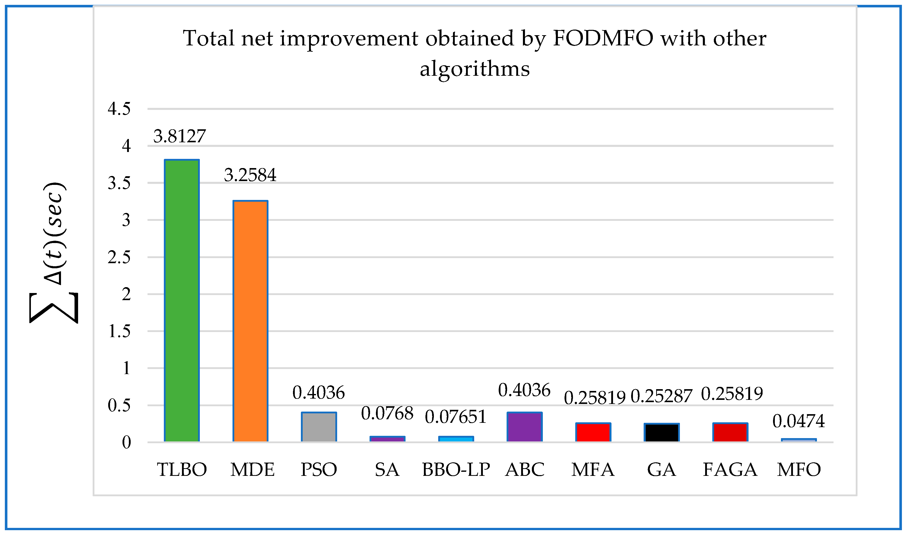
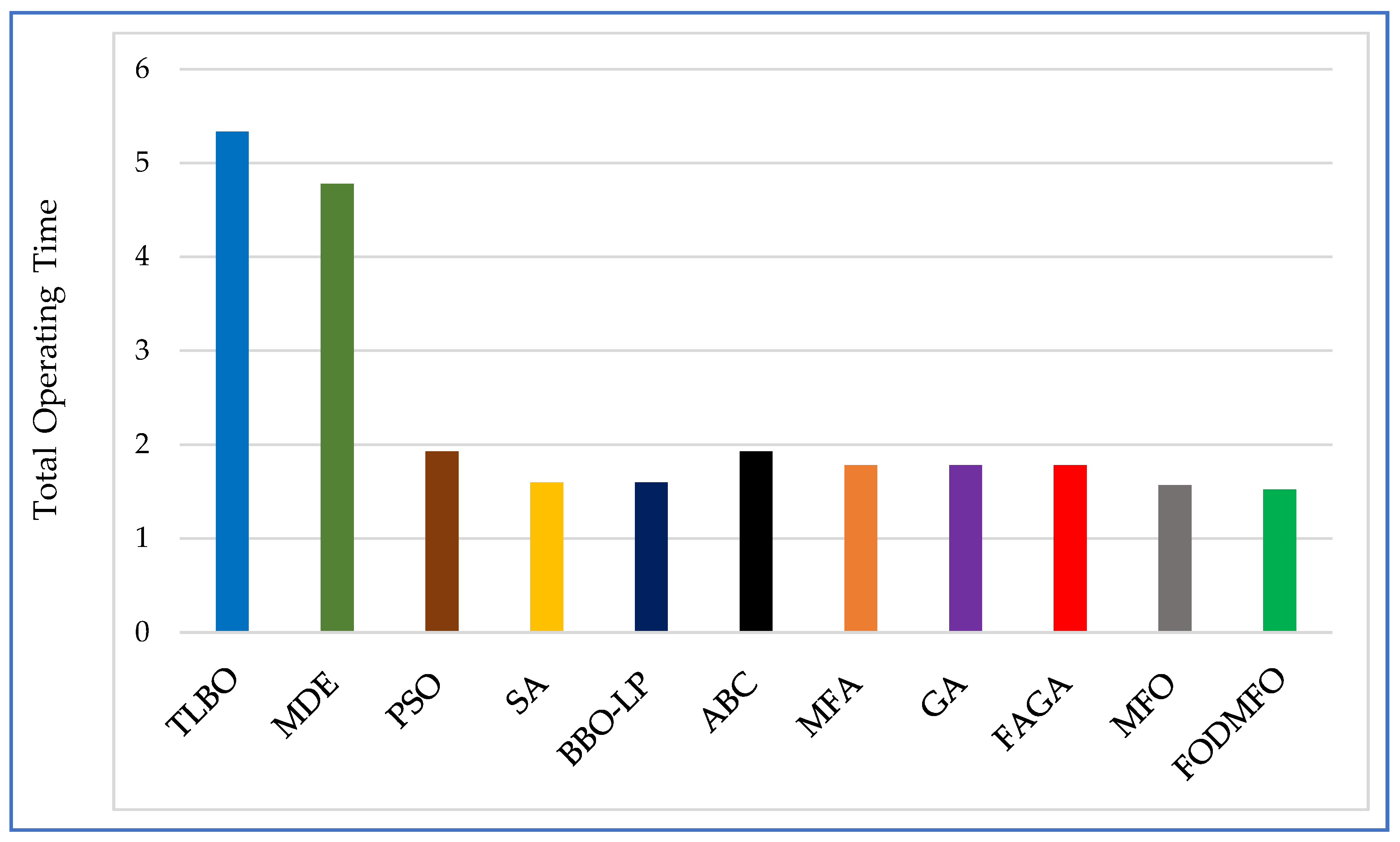
5. Comparative and Statistical Analysis

The MFO and FODMFO algorithms were implemented to solve the DOCR coordination issue for the IEEE benchmark 3, 8, and 15 bus systems. The obtained results obtained with the findings in the literature [4,6,13,20,22,31,32,33,34,39,41,42]. The suggested method obtained the optimal solution for resolving the issue in the DOCRs with the shortest possible response time. The findings validate that FODMFO has a greater capacity for fault detection and a faster rate of convergence in comparison to other optimization methodologies. Upon comparing the suggested FODMFO with all the strategies mentioned in the literature, it is evident that the proposed algorithm surpasses all other algorithms. For an accurate comparison with the other approaches, the same boundary conditions and parameters were used. The convergence characteristic graphs shown in Figure 4, Figure 9 and Figure 14 demonstrate that the convergence occurs more rapidly and reaches the optimal value with less iterations. For the IEEE 3-bus system, the total advantage in terms of net gain in total operating time is of 3.81 s compared to TLBO algorithms, 3.2584 s for MDE, 0.40 s for PSO, 0.07 s for SA and BBO-LP while 0.04 s is obtained for the MFO algorithm, respectively. In terms of percentage, there was a 71.4671% improvement observed in the TLBO algorithm, 68.15% in the MDE, 20.95% in the PSO, 4.80% in the SA and BBO-LP, and 3.01% in the MOF algorithm. The IEEE 8-bus system achieved a net gain of 2.34 s for GA, 2.40 s for LM, 2.744 s for BH, 3.1033 s for HS, 2.2 s for GA-LP, 1.89 s for BBO, and 1.57 s for JAYA. For DJAYA, OJAYA, MFO, and TLBO (MOF), a net gain of 1.30 s was obtained. These results correspond to percentage improvements of 21.30%, 20.94%, 21.76%, 24.07%, 26.38%, 17.94%, 15.4% and 13.13%, 12.13%, and 9.31%. In the IEEE 15-bus system, FODMFO yields a net gain over MINLP, BSA, MTLBO, GSO, GWO, EFO, ER-WCA, DJAYA, OJAYA, and MFO at 2.63 s, 3.59 s, 39.8 s, 1.25 s, 2.57 s. 5.20 s, 3.21 s, 6.14 s, 2.82 s, and 1.54 s, respectively. In this case, the comparison of optimal settings determined by FODMFO with MINLP, BSA, MTLBO, GSO, GWO, EFO, ER-WCA, DJAYA, OJAYA, and MFO shows 17.18%, 22.05%, 50.80%, 6.99%, 16.87%, 29.07%, 20.18%, 32.59%, 18.19%, and 10.85% improvement, respectively. The convergence figures obtained during the course of the simulation for all IEEE case studies reveal that the convergence rate is rapid, resulting in a satisfactory solution with few iterations. In order to assess the dependability, steadiness, and uniformity of the suggested FODMFO algorithm, a thorough statistical analysis was conducted on the IEEE 15-bus networks, taking into account the most feasible fractional order. In order to obtain accurate data, we performed 100 independent simulations and used the median of the final response as a reference point to determine the optimal fractional order. The statistical analysis relies on several tools such as the empirical cumulative distribution function, histograms, plots, box-plot demonstrations, quantile–quantile plots, and the minimal fitness development in each independent simulation, as shown in Figure 18a–e. Figure 18a demonstrates that the probability of finding an optimal solution using FODMFO is much greater than that using conventional MFO. The data shown in Figure 18b indicate that the median of the final solution in 100 trials tends to be lower for FODMFO compared to MFO. The histograms in Figure 18c illustrate that several trials resulted in the lowest fitness score. The suggested FODMFO has a very desirable minimal fitness when compared to the quantiles of the normal distribution, as seen in Figure 18d. The graph in Figure 18e demonstrates that FODMFO exhibits lower fitness levels than MFO throughout several independent executions. Considering these visual representations, it can be inferred that fractional calculus is a novel mathematical instrument that may be used to develop a modified version of traditional optimization approaches.

6. Conclusions

An innovative optimization methodology, FODMFO, is designed to solve the coordination issue in DOCRs in standard IEEE benchmark systems by using the concept of fractional calculus in the conventional MFO, making it an alternate, efficient, and precise solution. The proposed FODMFO aims to integrate the idea of fractional derivatives into the mathematical model of MFO, specifically focusing on the velocity update mechanism throughout each iteration. This collaboration has enhanced the optimization properties of the conventional method by accelerating the pace at which it reaches a solution and preventing it from prematurely converging. FODMFO is effectively evaluated in three distinct IEEE standard bus systems to reduce the overall operating time of DOCRs by adjusting the control parameters, such as the PS and TDS of the main and backup relays, to achieve near-optimal values. The results obtained by FODMFO are compared to those obtained from other recently developed algorithms such as TLBO, MDE, PSO, SA, BBO-LP, GA, BSA, MTLBO, GSO, GWO, EFO, ER-WCA, DJAYA, and others. The FODMFO algorithm has achieved superior performance compared to the algorithms stated earlier by substantially lowering the operational time of DOCRs in MINLP models in all case studies. This is an endorsement of FODMFO’s reliability, constancy, and stability, and is further supported by statistical analyses, such as cumulative distribution function plots, minimum fitness value plots, box-plots, standard normal quantile plots and histogram illustrations, and evolution in each independent simulation for the IEEE 15-bus system. The findings demonstrate that the combination of the fractional calculus tool with MFO has enhanced the optimizer’s performance in terms of rate of convergence speed during the MFO execution. The collected findings provide justification for the efficacy of FODMFO in identifying superior and optimal solutions for DOCRs, thereby demonstrating its effectiveness as a tool for relay coordination and optimization.

The proposed FODMFO will be utilized in the future on the protection coordination problem for micro-grids, both in grid-connected and islanded modes of operation. This includes line, substation, and distributed generation outages, as well as micro-grid operation modes.

References

1. Damborg, M.; Ramaswami, R.; Venkata, S.; Postforoosh, J. Computer aided transmission protection system design part I: Alcorithms. IEEE Trans. Power Appar. Syst. 1984, PAS-103, 51–59. [Google Scholar]
2. Birla, D.; Maheshwari, R.; Gupta, H. A New nonlinear directional overcurrent relay coordination technique, and banes and boons of near-end faults based approach. IEEE Trans. Power Deliv. 2006, 21, 1176–1182. [Google Scholar] [CrossRef]
3. Sharifian, H.; Abyaneh, H.A.; Salman, S.K.; Mohammadi, R.; Razavi, F. Determination of the minimum break point set using expert system and genetic algorithm. IEEE Trans. Power Deliv. 2010, 25, 1284–1295. [Google Scholar] [CrossRef]
4. Lu, Y.; Chung, J.-L. Detecting and solving the coordination curve intersection problem of overcurrent relays in subtransmission systems with a new method. Electr. Power Syst. Res. 2013, 95, 19–27. [Google Scholar] [CrossRef]
5. Ezzeddine, M.; Kaczmarek, R.; Iftikhar, M. Coordination of directional overcurrent relays using a novel method to select their settings. IET Gener. Transm. Distrib. 2011, 5, 743–750. [Google Scholar] [CrossRef]
6. Yu, J.; Kim, C.H.; Rhee, S.B. Oppositional Jaya algorithm with distance-adaptive coefficient in solving directional over current relays coordination problem. IEEE Access 2019, 7, 150729–150742. [Google Scholar] [CrossRef]
7. Khurshaid, T.; Wadood, A.; Farkoush, S.G.; Yu, J.; Kim, C.H.; Rhee, S.B. An improved optimal solution for the directional overcurrent relays coordination using hybridized whale optimization algorithm in complex power systems. IEEE Access 2019, 7, 90418–90435. [Google Scholar] [CrossRef]
8. Wadood, A.; Khurshaid, T.; Farkoush, S.G.; Yu, J.; Kim, C.H.; Rhee, S.B. Nature-inspired whale optimization algorithm for optimal coordination of directional overcurrent relays in power systems. Energies 2019, 12, 2297. [Google Scholar] [CrossRef]
9. Wadood, A.; Farkoush, S.G.; Khurshaid, T.; Yu, J.T.; Kim, C.H.; Rhee, S.B. Application of the JAYA Algorithm in Solving the Problem of the Optimal Coordination of Overcurrent Relays in Single-and Multi-Loop Distribution Systems. Complexity 2019, 2019, 5876318. [Google Scholar] [CrossRef]
10. Bhattacharya, S.K.; Goswami, S.K. Distribution network reconfiguration considering protection coordination constraints. Electr. Power Compon. Syst. 2008, 36, 1150–1165. [Google Scholar] [CrossRef]
11. Abyaneh, H.; Al-Dabbagh, M.; Karegar, H.; Sadeghi, S.; Khan, R. A new optimal approach for coordination of overcurrent relays in interconnected power systems. IEEE Trans. Power Deliv. 2003, 18, 430–435. [Google Scholar] [CrossRef]
12. Bedekar, P.P.; Bhide, S.R. Optimum coordination of directional overcurrent relays using the hybrid GA-NLP approach. IEEE Trans. Power Deliv. 2010, 26, 109–119. [Google Scholar] [CrossRef]
13. Noghabi, A.S.; Sadeh, J.; Mashhadi, H.R. Considering different network topologies in optimal overcurrent relay coordination using a hybrid GA. IEEE Trans. Power Deliv. 2009, 24, 1857–1863. [Google Scholar] [CrossRef]
14. Urdaneta, A.; Perez, L.; Restrepo, H. Optimal coordination of directional overcurrent relays considering dynamic changes in the network topology. IEEE Trans. Power Deliv. 1997, 12, 1458–1464. [Google Scholar] [CrossRef]
15. Noghabi, A.S.; Mashhadi, H.R.; Sadeh, J. Optimal coordination of directional overcurrent relays considering different network topologies using interval linear programming. IEEE Trans. Power Deliv. 2010, 25, 1348–1354. [Google Scholar] [CrossRef]
16. Najy, W.K.; Zeineldin, H.H.; Woon, W.L. Optimal protection coordination for microgrids with grid-connected and islanded capability. IEEE Trans. Ind. Electron. 2012, 60, 1668–1677. [Google Scholar] [CrossRef]
17. Saleh, K.A.; Zeineldin, H.H.; El-Saadany, E.F. Optimal protection coordination for microgrids considering N-1 contingency. IEEE Trans. Ind. Inform. 2017, 13, 2270–2278. [Google Scholar] [CrossRef]
18. Saleh, K.A.; Zeineldin, H.H.; Al-Hinai, A.; El-Saadany, E.F. Optimal coordination of directional overcurrent relays using a new time-current-voltage characteristic. IEEE Trans. Power Syst. 2014, 30, 537–544. [Google Scholar] [CrossRef]
19. Saleh, K.A.; El-Saadany, E.F.; Al-Hinai, A.; Zeineldin, H.H. Dual-setting characteristic for directional overcurrent relays considering multiple fault locations. IET Gener. Transm. Distrib. 2015, 9, 1332–1340. [Google Scholar] [CrossRef]
20. Korashy, A.; Kamel, S.; Alquthami, T.; Jurado, F. Optimal coordination of standard and non-standard direction overcurrent relays using an improved moth-flame optimization. IEEE Access 2020, 8, 87378–87392. [Google Scholar] [CrossRef]
21. Irfan, M.; Wadood, A.; Khurshaid, T.; Khan, B.M.; Kim, K.C.; Oh, S.R.; Rhee, S.B. An optimized adaptive protection scheme for numerical and directional overcurrent relay coordination using Harris hawk optimization. Energies 2021, 14, 5603. [Google Scholar] [CrossRef]
22. Amraee, T. Coordination of directional overcurrent relays using seeker algorithm. IEEE Trans. Power Deliv. 2012, 27, 1415–1422. [Google Scholar] [CrossRef]
23. Urdaneta, A.; Nadira, R.; Jimenez, L.P. Optimal coordination of directional overcurrent relays in interconnected power systems. IEEE Trans. Power Deliv. 1988, 3, 903–911. [Google Scholar] [CrossRef]
24. Wadood, A.; Farkoush, S.G.; Khurshaid, T.; Kim, C.-H.; Yu, J.; Geem, Z.W.; Rhee, S.-B. An optimized protection coordination scheme for the optimal coordination of overcurrent relays using a nature-inspired root tree algorithm. Appl. Sci. 2018, 8, 1664. [Google Scholar] [CrossRef]
25. Wadood, A.; Khurshaid, T.; Farkoush, S.G.; Kim, C.H.; Rhee, S.B. A bio-inspired rooted tree algorithm for optimal coordination of overcurrent relays. In International Conference on Intelligent Technologies and Applications; Springer: Singapore, 2018; pp. 188–201. [Google Scholar]
26. Wadood, A.; Kim, C.-H.; Khurshiad, T.; Farkoush, S.G.; Rhee, S.-B. Application of a continuous particle swarm optimization (CPSO) for the optimal coordination of overcurrent relays considering a penalty method. Energies 2018, 11, 869. [Google Scholar] [CrossRef]
27. Khurshaid, T.; Wadood, A.; Farkoush, S.G.; Kim, C.-H.; Cho, N.; Rhee, S.-B. Modified particle swarm optimizer as optimization of time dial settings for coordination of directional overcurrent relay. J. Electr. Eng. Technol. 2019, 14, 55–68. [Google Scholar] [CrossRef]
28. Habib, K.; Lai, X.; Wadood, A.; Khan, S.; Wang, Y.; Xu, S. Hybridization of PSO for the Optimal Coordination of Directional Overcurrent Protection Relays. Electronics 2022, 11, 180. [Google Scholar] [CrossRef]
29. Habib, K.; Lai, X.; Wadood, A.; Khan, S.; Wang, Y.; Xu, S. An improved technique of Hybridization of PSO for the Optimal Coordination of Directional Overcurrent Protection Relays of IEEE bus system. Energies 2022, 15, 3076. [Google Scholar] [CrossRef]
30. Mansour, M.M.; Mekhamer, S.F.; El-Kharbawe, N. A modified particle swarm optimizer for the coordination of directional overcurrent relays. IEEE Trans. Power Deliv. 2007, 22, 1400–1410. [Google Scholar] [CrossRef]
31. Thangaraj, R.; Pant, M.; Deep, K. Optimal coordination of over-current relays using modified differential evolution algorithms. Eng. Appl. Artif. Intell. 2010, 23, 820–829. [Google Scholar] [CrossRef]
32. Bouchekara, H.; Zellagui, M.; Abido, M.; Bouchekara, H.R.E.-H. Optimal coordination of directional overcurrent relays using a modified electromagnetic field optimization algorithm. Appl. Soft Comput. 2017, 54, 267–283. [Google Scholar] [CrossRef]
33. Khurshaid, T.; Wadood, A.; Farkoush, S.G.; Kim, C.H.; Yu, J.; Rhee, S.B. Improved firefly algorithm for the optimal coordination of directional overcurrent relays. IEEE Access 2019, 7, 78503–78514. [Google Scholar] [CrossRef]
34. Damchi, Y.; Dolatabadi, M.; Mashhadi, H.R.; Sadeh, J. MILP approach for optimal coordination of directional overcurrent relays in interconnected power systems. Electr. Power Syst. Res. 2018, 158, 267–274. [Google Scholar] [CrossRef]
35. Kim, C.H.; Khurshaid, T.; Wadood, A.; Farkoush, S.G.; Rhee, S.B. Gray wolf optimizer for the optimal coordination of directional overcurrent relay. J. Electr. Eng. Technol. 2018, 13, 1043–1051. [Google Scholar]
36. Albasri, F.A.; Alroomi, A.R.; Talaq, J.H. Optimal Coordination of directional overcurrent relays using biogeography-based optimization algorithm. IEEE Trans. Power Deliv. 2015, 30, 1810–1820. [Google Scholar] [CrossRef]
37. Singh, M.; Panigrahi, B.; Abhyankar, A. Optimal coordination of directional over-current relays using teaching learning-based optimization (TLBO) algorithm. Int. J. Electr. Power Energy Syst. 2013, 50, 33–41. [Google Scholar] [CrossRef]
38. El-Hana Bouchekara, H.R.; Zellagui, M.; Abido, M.A. Coordination of directional overcurret relays using the backtracking search algorithm. J. Electr. Syst. 2016, 12, 387–405. [Google Scholar]
39. Kalage, A.A.; Ghawghawe, N.D. Optimum coordination of directional overcurrent relays using modified adaptive teaching learning based optimization algorithm. Intell. Ind. Syst. 2016, 2, 55–71. [Google Scholar] [CrossRef]
40. Mahari, A.; Seyedi, H. An analytic approach for optimal coordination of overcurrent relays. IET Gener. Transm. Distrib. 2013, 7, 674–680. [Google Scholar] [CrossRef]
41. Alipour, M.; Teimourzadeh, S.; Seyedi, H. Improved group search optimization algorithm for coordination of directional overcurrent relays. Swarm Evol. Comput. 2015, 23, 40–49. [Google Scholar] [CrossRef]
42. Foqha, T.; Khammash, M.; Alsadi, S.; Omari, O.; Refaat, S.S.; Al-Qawasmi, K.; Elrashidi, A. Optimal coordination of directional overcurrent relays using hybrid firefly–genetic algorithm. Energies 2023, 16, 5328. [Google Scholar] [CrossRef]
43. Ghamisi, P.; Couceiro, M.S.; Benediktsson, J.A. A novel feature selection approach based on FODPSO and SVM. IEEE Trans. Geosci. Remote Sens. 2014, 53, 2935–2947. [Google Scholar] [CrossRef]
44. Ates, A.; Alagoz, B.B.; Kavuran, G.; Yeroglu, C. Implementation of fractional order filters discretized by modified fractional order darwinian particle swarm optimization. Measurement 2017, 107, 153–164. [Google Scholar] [CrossRef]
45. Couceiro, M.S.; Rocha, R.P.; Ferreira, N.F.; Machado, J.T. Introducing the fractional-order Darwinian PSO. Signal Image Video Process. 2012, 6, 343–350. [Google Scholar] [CrossRef]
46. Shahri, E.S.A.; Alfi, A.; Machado, J.T. Fractional fixed-structure H∞ controller design using augmented Lagrangian particle swarm optimization with fractional order velocity. Appl. Soft Comput. 2019, 77, 688–695. [Google Scholar] [CrossRef]
47. Machado, J.T.; Kiryakova, V. The chronicles of fractional calculus. Fract. Calc. Appl. Anal. 2017, 20, 307–336. [Google Scholar] [CrossRef]
48. Fan, Q.; Ma, Y.; Wang, P.; Bai, F. Otsu Image Segmentation Based on a Fractional Order Moth–Flame Optimization Algorithm. Fractal Fract. 2024, 8, 87. [Google Scholar] [CrossRef]
49. Zhu, Q.; Yuan, M.; Liu, Y.L.; Chen, W.D.; Chen, Y.; Wang, H.R. Research and application on fractional-order Darwinian PSO based adaptive extended Kalman filtering algorithm. IAES Int. J. Robot. Autom. 2014, 3, 245. [Google Scholar] [CrossRef]
50. Kuttomparambil Abdulkhader, H.; Jacob, J.; Mathew, A.T. Fractional-order lead-lag compensator-based multi-band power system stabiliser design using a hybrid dynamic GA-PSO algorithm. IET Gener. Transm. Distrib. 2018, 12, 3248–3260. [Google Scholar] [CrossRef]
51. Kosari, M.; Teshnehlab, M. Non-linear fractional-order chaotic systems identification with approximated fractional-order derivative based on a hybrid particle swarm optimization-genetic algorithm method. J. AI Data Min. 2018, 6, 365–373. [Google Scholar]
52. Khan, B.S.; Qamar, A.; Wadood, A.; Almuhanna, K.; Al-Shamma, A.A. Integrating economic load dispatch information into the blockchain smart contracts based on the fractional-order swarming optimizer. Front. Energy Res. 2024, 12, 1350076. [Google Scholar] [CrossRef]
53. Muhammad, Y.; Raja, M.A.Z.; Shah, M.A.A.; Awan, S.E.; Ullah, F.; Chaudhary, N.I.; Cheema, K.M.; Milyani, A.H.; Shu, C.M. Optimal coordination of directional overcurrent relays using hybrid fractional computing with gravitational search strategy. Energy Rep. 2021, 7, 7504–7519. [Google Scholar] [CrossRef]
54. Muhammad, Y.; Akhtar, R.; Khan, R.; Ullah, F.; Raja, M.A.Z.; Machado, J.T. Design of fractional evolutionary processing for reactive power planning with FACTS devices. Sci. Rep. 2021, 11, 593. [Google Scholar] [CrossRef]
55. Mirjalili, S. Moth-flame optimization algorithm: A novel nature-inspired heuristic paradigm. Knowl. Based Syst. 2015, 89, 228–249. [Google Scholar] [CrossRef]
56. Teodoro, G.S.; Machado, J.T.; De Oliveira, E.C. A review of definitions of fractional derivatives and other operators. J. Comput. Phys. 2019, 388, 195–208. [Google Scholar] [CrossRef]
57. Sabatier, J.A.T.M.J.; Agrawal, O.P.; Machado, J.T. Advances in Fractional Calculus; No. 9; Springer: Dordrecht, The Netherlands, 2007; Volume 4. [Google Scholar]
58. Razmjooei, H.; Shafiei, M.H.; Palli, G.; Arefi, M.M. Non-linear finite-time tracking control of uncertain robotic manipulators using time-varying disturbance observer-based sliding mode method. J. Intell. Robot. Syst. 2022, 104, 36. [Google Scholar] [CrossRef]
59. Abido, M.A. Power system stability enhancement using FACTS controllers: A review. Arab. J. Sci. Eng. 2009, 34, 153–172. [Google Scholar]
Figure 1. DOCR coordination in an electrical power network.
Fractalfract 08 00251 g001
Figure 2. Graphical representation of proposed methodology.
Fractalfract 08 00251 g002
Figure 3. Single line diagram of IEEE 3-bus system.
Fractalfract 08 00251 g003
Figure 4. Convergence characteristic graph case 1.
Fractalfract 08 00251 g004
Figure 5. Comparative analysis of net improvement in total operating time (s).
Fractalfract 08 00251 g005
Figure 6. Comparative analysis in percentage improvement in net gain compared to other algorithms for IEEE 3-bus system.
Fractalfract 08 00251 g006
Figure 7. Optimized total operating time: FODMFO vs. literature for IEEE 3-bus system.
Fractalfract 08 00251 g007
Figure 8. Single-line diagram of IEEE 8-bus system.
Fractalfract 08 00251 g008
Figure 9. Convergence characteristics for MFO and FODMFO for IEEE 8-bus system.
Fractalfract 08 00251 g009
Figure 10. Comparative analysis of net improvement in total operating time (s), IEEE 8-bus system.
Fractalfract 08 00251 g010
Figure 11. Comparative analysis of percentage improvement in net gain compared to other algorithms, IEEE 8-us system.
Fractalfract 08 00251 g011
Figure 12. Optimized total operating time: FODMFO vs. literature for IEEE 8-bus system.
Fractalfract 08 00251 g012
Figure 13. Single-line diagram of IEEE 15-bus system.
Fractalfract 08 00251 g013
Figure 14. Convergence characteristics for MFO and FODMFO for IEEE 15-bus system.
Fractalfract 08 00251 g014
Figure 15. Comparative analysis of net improvement in total operating time (s) for IEEE 15-bus system.
Fractalfract 08 00251 g015
Figure 16. Comparative analysis in percentage improvement in net gain compared to other algorithms IEEE 15-bus system.
Fractalfract 08 00251 g016
Figure 17. Optimized total operating time: FODMFO vs. literature for IEEE 15-bus system.
Fractalfract 08 00251 g017
Figure 18. FODMFO comparison with MFO during time of operation minimization in MINLP model of IEEE 15-bus system. (a) CDF; (b) box-plot illustration; (c) histogram; (d) quantile–quantile plot; (e) minimum fitness.
Fractalfract 08 00251 g018