Article

Existence and Uniqueness Result for Fuzzy Fractional Order Goursat Partial Differential Equations

by
Muhammad Sarwar
1,2,*,
Noor Jamal
1,
Kamaleldin Abodayeh
2,
Chanon Promsakon
3,4,* and
Thanin Sitthiwirattham
4,5
1
Department of Mathematics, University of Malakand, Chakdara 18000, Dir(L) Khyber Pakhtunkhwa, Pakistan
2
Department of Mathematics and Sciences, Prince Sultan University, Riyadh 11586, Saudi Arabia
3
Department of Mathematics, Faculty of Applied Science, King Mongkut’s University of Technology North, Bangkok 10800, Thailand
4
Research Group for Fractional Calculus Theory and Applications, Science and Technology Research Institute, King Mongkut’s University of Technology North Bangkok, Bangkok 10800, Thailand
5
Mathematics Department, Faculty of Science and Technology, Suan Dusit University, Bangkok 10300, Thailand
*
Authors to whom correspondence should be addressed.
Submission received: 3 March 2024 / Revised: 6 April 2024 / Accepted: 13 April 2024 / Published: 25 April 2024

Abstract

:
In this manuscript, we discuss fractional fuzzy Goursat problems with Caputo’s g H -differentiability. The second-order mixed derivative term in Goursat problems and two types of Caputo’s g H -differentiability pose challenges to dealing with Goursat problems. Therefore, in this study, we convert Goursat problems to equivalent systems fuzzy integral equations to deal properly with the mixed derivative term and two types of Caputo’s g H -differentiability. In this study, we utilize the concept of metric fixed point theory to discuss the existence of a unique solution of fractional fuzzy Goursat problems. For the useability of established theoretical work, we provide some numerical problems. We also discuss the solutions to numerical problems by conformable double Laplace transform. To show the validity of the solutions we provide 3D plots. We discuss, as an application, why fractional partial fuzzy differential equations are the generalization of usual partial fuzzy differential equations by providing a suitable reason. Moreover, we show the advantages of the proposed fractional transform over the usual Laplace transform.

1. Introduction

The concept of dealing with fuzzyness in real life was initiated in the work of paper [1]. Classical calculus has been extended to fuzzy and fuzzy fractional calculus for the last two decades. The attention of many mathematicians to modern fuzzy and fuzzy fractional calculus is due to their significant applications, realistic description of physical, optimization, linear programming, banking industry, and biological problems. To optimize path length and energy consumption of robot routing [2], we use the fuzzy concept. The use of fuzzy concepts in the data analysis in banking [3], medical resources allocation [4], decision-making model for the operating system, and human–computer interaction [5], etc., show the importance of fuzzy calculus. Also, the uncertainty in physical models is dealt with easily in the fuzzy models [6,7].
Partial differential equations (PDEs) deal more with real-life problems than ordinary differential equations (DEs) because, during the study of natural phenomena, we often face several variables simultaneously. However, due to uncertainty, PDEs sometimes face difficulty in the study of physical problems. To remove this drawback, the paper [8] introduced the fuzzy PDEs (FPDEs). In this direction, many researchers share their contributions, and the fuzzy models on heat [9,10], advection-diffusion [11,12], and the Goursat problem [13] stem from these.
The generalization of integer order of differential and integral operators to real order generalized classical calculus to fractional calculus. Moreover, integer order differential operators are particular cases of the fractional order. Therefore, researchers show more interest in fractional order differential and integral equations. Salahshour et al. [14] extend the gH-differentiability to fuzzy fractional differentiability. In the papers [15,16,17], the existence and solutions of DEs with fuzzy fractional differentiability were discussed. Some fractional order problems are also studied in [18,19,20,21,22] and the references cited therein.
The Goursat problems have a second-order hyperbolic partial differential equation with mixed derivative terms. This problem arises in the wave phenomena with mixed derivatives. The Goursat problems are different from the other second-order partial differential equations like diffusion, advection-diffusion, and reaction-diffusion equations due to the mixed derivative term. The Goursat problems have important applications in different fields. Therefore, different solutions, processes, and applications of Goursat problems were discussed in [23,24,25,26]. The existing conditions of Goursat problems with fuzzy boundary conditions were discussed by [13].
In this manuscript, we discuss the Goursat problems with fuzzy boundary conditions and Caputo’s gH-differentiability concept. A fuzzy function is Caputo’s gH-differentiable if it is [ i g H ] C differentiable or [ i i g H ] C differentiable. The second-order FPDEs with gH-differentiability pose challenges due to two types of Caputo’s gH-differentiability. The Goursat problems are partial differential equations with the second-order term having mixed derivatives. Keeping these difficulties in mind, we study three aspects of these problems. First of all, we convert the fractional order Goursat problem to equivalent systems of fuzzy fractional integral equations to deal properly with the two types of Caputo’s gH-differentiability in the mixed derivative term. Next, we show that the equivalent systems of fuzzy fractional integral equations satisfy the FPDE and boundary conditions of the Goursat problem. After that, the results for the existence of unique solutions to fractional fuzzy Goursat problems are the goal of this study. In addition to theoretical proofs, in this manuscript, we discuss numerical examples. We discuss the solutions of numerical examples by conformable double Laplace transform. The manuscript also presents 3D fuzzy plots of solutions to illustrate our findings. In the last, we discuss why fractional FPDEs are the globalization of usual PDEs. We also investigate the advantages of fractional transform on the usual Laplace transform.

2. Preliminaries

Here, we revisit specific findings of the fuzzy and fuzzy fractional calculus. The fuzzy set A is a fuzzy number if it satisfies the following properties for all l , m , n , p R ;
( i )
A is upper semi-continuous;
( i i )
A is convex, i.e., ϑ [ 0 , 1 ] , A ( ϑ m + ( 1 ϑ ) n ) min A ( m ) , A ( n ) ;
( i i i )
A is normal, i.e., A ( p ) = 1 ;
( i v )
Closure of set { l R A ( l ) > 0 } is compact.
The set of all F-numbers is fuzzy space, denoted by R F .
The α -level set is [ A ] α = { a R | A ( a ) α } where [ A ] α = [ A ̲ α , A ¯ α ] R F for all 0 α 1 [27].
Definition 1 
([28]). The d F : R F × R F R + { 0 } is metric define in term of Hausdorff distance
d F ( x , y ) = sup α [ 0 , 1 ] d ( x α , y α ) = sup α [ 0 , 1 ] max | x ̲ α y ̲ α | , | x ¯ α y ¯ α | .
The complete metric space ( d F , R F ) has the following properties for all a , x , y , z R F .
D 1 ) d F ( x + z , y + z ) = d F ( x , y ) ; D 2 ) d F ( α x , α y ) = α d F ( x , y ) ; D 3 ) d F ( x + a , y + z ) d F ( x , y ) + d F ( a , z ) .
In this manuscript, I = ( a , b ) and J = ( c , d ) are open intervals of real numbers
Definition 2 
([28]). The χ : I R F is continuous if for ϵ > 0 , δ > 0 and arbitrarily fixed x 0 R hold the condition
| x x 0 | < δ d F ( χ ( x ) , χ ( x 0 ) ) < ϵ .
Corollary 1 
([28]). The function χ : I R F is integrable if it is continuous.
Remark 1 
([28]). If A : I R F is integrable and [ A ( ϑ ) ] α = [ A ̲ α ( ϑ ) , A ¯ α ( ϑ ) ] then [ A ( ϑ ) ] α = [ A ̲ α ( ϑ ) , A ¯ α ( ϑ ) ] .
Lemma 1 
([27]). If A , B : I R F is integrable and κ R then
( i )
( A + B ) = A + B .
( i i )
κ A = κ A .
( i i i )
d F ( A , B ) is integrable in interval I .
( i v )
d F ( A , B ) d F ( A , B ) .
Definition 3 
([29]). Let A , B , C R F then g H - difference of A , B is define by
A g H B = C A = B C , B = A ( C ) .
If the H - difference A B exist then A B = A g H B .
Definition 4 
([9,30]). The partial gH-differentiability of U : I × J R F , with respect to τ exist at the point ( τ , ω ) I × J if one of the following conditions holds
( i )
The H-difference U ( τ + δ , ω ) U ( τ , ω ) ,   U ( τ , ω ) U ( τ δ , ω ) exist for sufficiently small δ > 0 and the folloing limits exist in ( d F , R F ) .
lim δ 0 + U ( τ + δ , ω ) U ( τ , ω ) δ = lim δ 0 + U ( τ , ω ) U ( τ δ , ω ) δ = D τ i U ( τ , ω ) .
( i i )
The H-difference U ( τ , ω ) U ( τ + δ , ω ) , U ( τ δ , ω ) U ( τ , ω ) exist for sufficiently small δ > 0 and the following limits exist in ( d F , R F ) .
lim δ 0 + U ( τ , ω ) U ( τ + δ , ω ) ( δ ) = lim δ 0 + U ( τ δ , ω ) U ( τ , ω ) ( δ ) = D τ i i ( τ , ω ) .
The first one D i τ ( τ , ω ) is referred to [ i g H ] differentiable and second one D τ i i ( τ , ω ) to [ i i g H ) differentiable.
Lemma 2 
([9,30]). Let U : I × J R F , is a continuous function and [ U ( τ , ω ) ] α = [ U ̲ α ( τ , ω ) , U ¯ α ( τ , ω ) ] with 0 α 1 . Then for ( τ , ω ) I × J one can have
( i )
If [ D τ i U ( τ , ω ) ] α exist on I × J , then D τ i U ( τ , ω ) α = D τ U ̲ α ( τ , ω ) , D τ U ¯ α ( τ , ω ) .
( i i )
If [ D ω i U ( τ , ω ) ] α exist on I × J , then D ω i U ( τ , ω ) α = D ω U ̲ α ( τ , ω ) , D ω U ¯ α ( τ , ω ) .
( i i i )
If [ D τ i i U ( τ , ω ) ] α exist on I × J , then D τ i i U ( τ , ω ) α = D τ U ¯ α ( τ , ω ) , D τ U ̲ α ( τ , ω ) .
( i v )
If [ D ω i i U ( τ , ω ) ] α exist on I × J , then D ω i i U ( τ , ω ) α = D ω U ¯ α ( τ , ω ) , D ω U ̲ α ( τ , ω ) .
Definition 5 
([13]). Let u : I × J F R be a fuzzy function. If for k , l { i , i i } the D x k u and D y l u exists on I × J . Then, u is second-order partial [ k g H ] differentiable with respect to x at ( x 0 , y 0 ) { x 0 } × I and [ l g H ] differentiable with respect to y at ( x 0 , y 0 ) { x 0 } × J .
Let us denote the partial second-order [k,l-gH]differentiability of u with respect to x , y at ( x 0 , y 0 ) by D x y k , l u ( x 0 , y 0 ) , where k , l { i , i i } . Similarly, we have D x x k , l u ,   D y x k , l u ,   D y y k , l u . For k = l where k , l { i , i i } one can write D x y k u ,   D x x k u ,   D x y k u and D y y k u .
Lemma 3 
([13]). Let χ : I × J R F is continuous and [ χ ( τ , ω ) ] α = [ χ ̲ α ( τ , ω ) , χ ¯ α ( τ , ω ) ] and 0 α 1 such that D τ ω k , l χ ( τ , ω ) exist on I × J , then
( i )
[ D τ ω k , l χ α ( τ , ω ) ] = [ D τ ω χ ̲ α ( τ , ω ) , D τ ω χ ¯ α ( τ , ω ) ] if k = l where k , l { i , i i } .
( i i )
[ D τ ω k , l χ α ( τ , ω ) ] = [ D τ ω χ ¯ α ( τ , ω ) , D τ ω χ ̲ α ( τ , ω ) ] if k l where k , l { i , i i } .
Lemma 4 
([28]). Let χ : I R F is g H -differentiable at s I and derivative χ : I R F is continuous at each s I then
d F ( χ ( s ) , χ ( t ) ) ( t s ) max x [ s , t ] d F ( χ ( x ) , t ) , for all s , t I with s < t .
The space C ( k , l ) I × J , R F consist of u : I × J R F such that [ u ( s , t ) ] α = [ u ̲ α ( s , t ) , u ¯ α ( s , t ) ] then v ( s , t ) = D s k u ( s , t ) and w ( s , t ) = D t l u ( s , t ) are continuous. Now, according to Lemma 3 one can write
[ v ( s , t ) ] α = [ D s k u ( s , t ) ] α = [ D s u ̲ α ( s , t ) , D s u ¯ α ( s , t ) ] , if k = i , [ D s u ¯ α ( s , t ) , D s u ̲ α ( s , t ) ] , if k = i i .
and
[ w ( s , t ) ] α = [ D t l u ( s , t ) ] α = [ D t u ̲ α ( s , t ) , D t u ¯ α ( s , t ) ] , if l = i , [ D t u ¯ α ( s , t ) , D t u ̲ α ( s , t ) ] , if l = i i .
Also for k , l { i , i i } and ( s , t ) I × J .
[ D s t l , k u ( s , t ) ] α = [ D t l v ( s , t ) ] α = [ D s t u ̲ α ( s , t ) , D s t u ¯ α ( s , t ) ] , if l = k .
[ D t s l , k u ( s , t ) ] α = [ D s k w ( s , t ) ] α = [ D t s u ¯ α ( s , t ) , D t s u ̲ α ( s , t ) ] , if l = k .
and
[ D s t l , k u ( s , t ) ] α = [ D t l v ( s , t ) ] α = [ D s t u ̲ α ( s , t ) , D s t u ¯ α ( s , t ) ] , if l k .
[ D t s l , k u ( s , t ) ] α = [ D s k w ( s , t ) ] α = [ D t s u ¯ α ( s , t ) , D t s u ̲ α ( s , t ) ] , if l k .
Lemma 5 
([13]). Let u : ( 0 , S ) × ( 0 , T ) F R be defined in the neighborhood ( 0 , S ) × ( 0 , T ) R 2 of point ( τ , ω ) R 2 . Assume that D τ i u ,   D ω i u ,   D τ ω i u exist in ( 0 , S ) × ( 0 , T ) ,   D τ i u ( τ , ω ) be continuous on τ(for fixed ω) D ω i u ( τ , ω ) be continuous on ω(for fixed τ) and D τ ω i u be continuous at ( τ , ω ) . If for all τ ( 0 , S ) the following H-Differences exist close enough to τ .
u ( τ + κ , ω + δ ) u ( τ + κ , ω ) u ( τ , ω + δ ) u ( τ , ω ) κ δ D τ ω i u ( τ , ω ) ,
u ( τ , ω + δ ) u ( τ , ω ) u ( τ κ , ω + δ ) u ( τ κ , ω ) κ δ D τ ω i u ( τ , ω ) ,
u ( τ , ω ) u ( τ , ω δ ) u ( τ κ , ω ) u ( τ κ , ω κ ) κ δ D τ ω i u ( τ , ω ) ,
u ( τ + κ , ω ) u ( τ + κ , ω δ ) u ( τ , ω ) u ( τ , ω κ ) κ δ D τ ω i u ( τ , ω ) .
And for all ω ( 0 , T ) the following H-Differences exist close enough to ω .
D τ i u ( τ + z , ω + δ ) D τ i u ( τ + z , ω ) δ D τ ω i u ( τ , ω ) ,
D τ i u ( τ + z , ω ) D τ i u ( τ + z , ω δ ) δ D τ ω i u ( τ , ω ) ,
D τ i u ( τ z , ω + δ ) D τ i u ( τ z , ω ) δ D τ ω i u ( τ , ω ) ,
D τ i u ( τ z , ω ) D τ i u ( τ z , ω δ ) δ D τ ω i u ( τ , ω ) ,
For z [ 0 , κ ] and κ , δ > 0 small enough that D τ ω i u ( τ , ω ) exist and D τ ω i u ( τ , ω ) = D ω τ i u ( τ , ω ) .
Remark 2 
([13]). Since D τ i exist in ( 0 , S ) × ( 0 , T ) R 2 , then u ( τ + κ , ω + δ ) u ( τ , ω + δ ) u ( τ + κ , ω ) u ( τ , ω ) exist for κ , δ > 0 enough small. The H-Differences
u ( τ + κ , ω + δ ) u ( τ + κ , ω ) u ( τ , ω + δ ) u ( τ , ω ) ,
u ( τ + κ , ω + δ ) u ( τ , ω + δ ) u ( τ + κ , ω ) u ( τ , ω ) ,
exist and u ( τ + κ , ω + δ ) u ( τ + κ , ω ) u ( τ , ω + δ ) u ( τ , ω ) = u ( τ + κ , ω + δ ) u ( τ , ω + δ ) u ( τ + κ , ω ) u ( τ , ω ) . Using Lemma 5 one can obtain
lim ( κ , δ ) ( 0 + , 0 + ) u ( τ + κ , ω + δ ) u ( τ + κ , ω ) u ( τ , ω + δ ) u ( τ , ω ) κ δ = D ω τ i u ( τ , ω ) .
Similarly
lim ( κ , δ ) ( 0 + , 0 + ) u ( τ + κ , ω + δ ) u ( τ , ω + δ ) u ( τ + κ , ω ) u ( τ , ω ) κ δ = D ω τ i u ( τ , ω )
Definition 6 
([31]). Let u ( τ ) be a function, the integral of fractional order is defined as
I θ u ( τ ) = 1 Γ ( θ ) 0 τ ( τ ω ) θ 1 u ( ω ) d ω , θ > 0 ,
Definition 7 
([31]). Caputo’s derivative of u ( t ) is defined as
D θ C u ( t ) = 1 Γ ( n θ ) 0 t ( t ζ ) n θ 1 [ u n ( ζ ) ] d ζ , θ > 0 .
Definition 8 
([15]). Caputo’s gH-differentiability of fuzzy valued function u C F [ 0 , b ] L F [ 0 , b ] is defined as
D a + θ g H C u ( t ) = 1 Γ ( 1 θ ) a t ( t s ) θ u ( s ) d s
( i )
u is said to be [ i g H ] C differentiable if Equation (1) holds and u is ( i ) -differentiable.
( i i )
u is said to be [ i i g H ] C differentiable if Equation (1) holds and u is ( i i ) -differentiable.
Lemma 6 
([15]). Let function u C F [ a , b ] , then for 0 < θ 1
( i )
If u is [ ( i ) g H ] C differentiable then I a + θ g H C ( D a + θ g H C u ( t ) ) = u ( t ) g H u ( a ) .
( i i )
If u is [ ( i i ) g H ] C differentiable then I a + θ g H C ( D a + θ g H C u ( t ) ) = u ( a ) g H ( 1 ) u ( t ) .
Lemma 7 
([14]). Let us have the following equation with 0 < θ 1
D a + θ g H C u ( x ) = f ( x , u ( x ) ) , u ( a ) F R .
( i )
If u is [ i g H ] C differentiable, then the equivalent integral form is
u ( x ) = u ( a ) + 1 Γ ( θ ) a x ( x z ) θ 1 f ( z , u ( z ) ) d z
( i i )
If u is [ i i g H ] C differentiable, then the equivalent integral form is
u ( x ) = u ( a ) 1 Γ ( θ ) a x ( x z ) θ 1 f ( z , u ( z ) ) d z
Definition 9 
([32]). Let Caputo’s fractional derivative of u C F [ 0 , b ] L F [ 0 , b ] with u = [ u ̲ α ( t ) , u ¯ α ( t ) ] , α [ 0 , 1 ] and t 0 ( 0 , b ) be defined as
[ C D θ u ( t 0 ) ] α = [ C D θ u ̲ α ( t 0 ) , C D θ u ¯ α ( t 0 ) ] ,
where
D θ C u ̲ α ( t 0 ) = 1 Γ ( n θ ) 0 t ( t ζ ) n θ 1 d n d ζ n u ̲ α ( ζ ) d ζ t = t 0 . D θ C u ¯ α ( t 0 ) = 1 Γ ( n θ ) 0 t ( t ζ ) n θ 1 d n d ζ n u ¯ α ( ζ ) d ζ t = t 0 .
where n = [ θ ] with θ ( 0 , 1 ] .
Definition 10 
([31]). The Mittag–Leffler function E γ , β of two parametric forms is defined in the series form as follows
E γ , β ( v ) = k = 0 v k Γ ( γ k + β )
where γ > 0 ,   β > 0 . Integrating (3) term-by-term, we obtain
0 t E γ , β ( λ v γ ) v β 1 d v = t γ E γ , β + 1 ( λ t γ ) , ( β > 0 ) .
Definition 11 
([33]). The conformable Laplace transform(CLT) with respect to τ of u ( τ , ω ) is given as
L τ θ u ( τ , ω ) = u ( s , ω ) = 0 e s τ θ θ u ( τ , ω ) d θ τ .
Lemma 8 
([33]). θ-th order conformable Laplace transform(CLT) of order 0 < θ 1 is define as
L θ d θ y ˜ ( τ ) d τ θ = s [ y ˜ ( τ ) ] [ y ˜ ( 0 ) ] .

3. Existence and Uniqueness Results of Fractional Order Fuzzy Goursat Problem

Now, we discuss an existing result for a unique solution of the fractional order fuzzy Goursat problem.
Let us consider the following fractional FDEs of order 0 < θ 1 .
D x y k , l θ u ( x , y ) = a 1 D x k θ u ( x , y ) + a 2 D y l θ u ( x , y ) + a 3 u ( x , y ) + G ( x , y ) , u ( x , 0 ) = ϕ 1 ( x ) , 0 x x 0 , u ( 0 , y ) = ϕ 2 ( y ) , 0 y y 0 , ϕ 1 ( 0 ) = ϕ 2 ( 0 ) .
Such that a 1 , a 2 , a 3 , G : Y R are continuous on the close rectangle Y = [ 0 , x 0 ] × [ 0 , y 0 ] where ϕ 1 ( x ) : [ 0 , x 0 ] F R and ϕ 2 ( y ) : [ 0 , y 0 ] F R are also continuous and k , l { i , i i } . We search for solution u ( x , y ) C ( k , l ) ( Y , F R ) .
Definition 12. 
The fuzzy valved function, u C ( k , l ) ( Y , F R ) is the solution of Equation (7) if u ( x , y ) satisfies problem (7).
Let u C ( k , l ) ( Y , F R ) be the solution of Equation (7) such that D x y ( k , l ) θ u ( x , y ) ,   D y x k , l θ u ( x , y ) exist and D x y k , l θ u ( x , y ) = D y x k , l θ u ( x , y ) . We convert Equation (7) to the following equivalent systems. For this put D x k θ u ( x , y ) = v ( x , y ) , D y l θ u ( x , y ) = w ( x , y ) where v , w : Y F R are continuous fuzzy functions. Therefore, we deduce
D x k θ w ( x , y ) = D y l θ v ( x , y ) = a 1 v ( x , y ) + a 2 w ( x , y ) + a 3 u ( x , y ) + G ( x , y ) , v ( x , 0 ) = D y k θ ϕ 1 ( x ) , 0 x x 0 , w ( 0 , y ) = D y l θ ϕ 2 ( y ) , 0 y y 0 .
Using, Lemma 7 and initial condition we have
1:
For k = l = i , the following system of equations is obtained
u ( x , y ) = ϕ 1 ( x ) + 1 Γ θ 0 y ( y y ) θ 1 w ( x , y ) d y , v ( x , y ) = D x i θ ϕ 1 ( x ) + 1 Γ θ 0 y ( y y ) θ 1 ( a 1 v + a 2 w + a 3 u + G ) ( x , y ) d y , w ( x , y ) = D y i θ ϕ 2 ( y ) + 1 Γ θ 0 x ( x x ) θ 1 ( a 1 v + a 2 w + a 3 u + G ) ( x , y ) d x .
2:
For k = i and l = i i , the following system of equations is obtained
u ( x , y ) = ϕ 1 ( x ) + 1 Γ θ 0 y ( y y ) θ 1 w ( x , y ) d y , v ( x , y ) = D x i θ ϕ 1 ( x ) + 1 Γ θ 0 y ( y y ) θ 1 ( a 1 v + a 2 w + a 3 u + G ) ( x , y ) d y , w ( x , y ) = D y i i θ ϕ 2 ( y ) ( 1 ) 1 Γ θ 0 x ( x x ) θ 1 ( a 1 v + a 2 w + a 3 u + G ) ( x , y ) d x .
3:
For k = i i and l = i , the following system of equations is obtained
u ( x , y ) = ϕ 1 ( x ) + 1 Γ θ 0 y ( y y ) θ 1 w ( x , y ) d y , v ( x , y ) = D x i i θ ϕ 1 ( x ) ( 1 ) 1 Γ θ 0 y ( y y ) θ 1 ( a 1 v + a 2 w + a 3 u + G ) ( x , y ) d y , w ( x , y ) = D y i θ ϕ 2 ( y ) + 1 Γ θ 0 x ( x x ) θ 1 ( a 1 v + a 2 w + a 3 u + G ) ( x , y ) d x .
4:
For k = l = i i , the following system of equations is obtained
u ( x , y ) = ϕ 1 ( x ) ( 1 ) 1 Γ θ 0 y ( y y ) θ 1 w ( x , y ) d y , v ( x , y ) = D x i i θ ϕ 1 ( x ) ( 1 ) 1 Γ θ 0 y ( y y ) θ 1 ( a 1 v + a 2 w + a 3 u + G ) ( x , y ) d y , w ( x , y ) = D y i i θ ϕ 2 ( y ) ( 1 ) 1 Γ θ 0 x ( x x ) θ 1 ( a 1 v + a 2 w + a 3 u + G ) ( x , y ) d x .
Conversely, let us suppose the functions u ( x , y ) ,   v ( x , y ) and w ( x , y ) are continuous on Y and satisfying one of the system (9)–(12). We have to show that a solution u ( x , y ) to the system of integral equations is the solution to the problem (7) and u C ( k , l ) ( Y , F R ) .
Using Lemma 6 and Equation (9), we deduce Equation (8) and D y i θ u ( x , y ) = w ( x , y ) . Then, w ( x , y ) = D y i θ ϕ 2 ( y ) + 1 Γ θ 0 x ( x x ) θ 1 ( a 1 v + a 2 w + a 3 u + G ) ( x , y ) d x is [ i g H ] C differentiable with respect to x . Therefore
D x i θ I y θ w ( x , y ) d y = D x i θ I y θ D y i θ ϕ 2 ( y ) + 1 Γ θ 0 x ( x x ) θ 1 ( a 1 v + a 2 w + a 3 u + G ) ( x , y ) d x d y , = D x i θ I y θ D y i θ ϕ 2 ( y ) + D x i θ { I y θ 1 Γ θ 0 x ( x x ) θ 1 ( a 1 v + a 2 w + a 3 u + G ) ( x , y ) d x d y } , = D x i θ I y θ D y i θ ϕ 2 ( y ) + D x i θ { I y θ 1 Γ θ 0 x ( x x ) θ 1 ( a 1 v + a 2 w + a 3 u + G ) ( x , y ) d x } d y , = D x i θ I y θ 1 Γ θ 0 x ( x x ) θ 1 ( a 1 v + a 2 w + a 3 u + G ) ( x , y ) d x d y , = 1 Γ θ 0 y ( y y ) θ 1 ( a 1 v + a 2 w + a 3 u + G ) ( x , y ) d y
Now, on the other hand
I y θ D x i θ w ( x , y ) d y = I y θ D x i θ D y i θ ϕ 2 ( y ) + 1 Γ θ 0 x ( x x ) θ 1 ( a 1 v + a 2 w + a 3 u + G ) ( x , y ) d x d y , = I y θ D x i θ D y i θ ϕ 2 ( y ) + I y θ ( D x i { 1 Γ θ 0 x ( x x ) θ 1 ( a 1 v + a 2 w + a 3 u + G ) ( x , y ) d x } ) d y , = I y θ D x i θ D y i θ ϕ 2 ( y ) + I y θ { D x i θ 1 Γ θ 0 x ( x x ) θ 1 ( a 1 v + a 2 w + a 3 u + G ) ( x , y ) d x } d y ,
= D y θ D x i θ 1 Γ θ 0 x ( x x ) θ 1 ( a 1 v + a 2 w + a 3 u + G ) ( x , y ) d x d y , = 1 Γ θ 0 y ( y y ) θ 1 ( a 1 v + a 2 w + a 3 u + G ) ( x , y ) d y .
From above we can obtain
D x i θ I y θ w ( x , y ) d y = I y θ D x i θ w ( x , y ) d y
From Equations (8), (9) and (13) and Remark 1 for k = l = i , we deduce
D x i θ u ( x , y ) = D x i θ ϕ 1 ( x ) + D x i θ 1 Γ θ 0 y ( y y ) θ 1 w ( x , y ) d y , = D x i θ ϕ 1 ( x ) + D x i θ ( I y θ w ( x , y ) d y ) , = D x i θ ϕ 1 ( x ) + 1 Γ θ 0 y ( y y ) θ 1 ( a 1 v + a 2 w + a 3 u + G ) ( x , y ) d y , = v ( x , y ) ( x , y ) Y .
Now, we show that u ( x , y ) C ( i , i ) ( Y , F R ) is a solution of Problem (7).
D y x i θ u ( x , y ) = D x i θ w ( x , y ) = ( a 1 v + a 2 w + a 3 u + G ) ( x , y ) = D y i θ v ( x , y ) = D x y i θ u ( x , y ) .
By Equation (9), u ( x , y ) satisfies the boundary conditions of Problem (7)
u ( x , y ) | y = 0 = ϕ 1 ( x ) , 0 x x 0 , 0 y y 0 . u ( x , y ) | x = 0 = ϕ 1 ( 0 ) + 1 Γ θ 0 y ( y y ) θ 1 w ( 0 , y ) d y = ϕ 1 ( 0 ) + 1 Γ θ 0 y ( y y ) θ 1 D y i θ ϕ 2 ( y ) d y = ϕ 1 ( 0 ) + ϕ 2 ( y ) ϕ 2 ( 0 ) = ϕ 2 ( y ) , 0 x x 0 , 0 y y 0 .
Now, we take the case k = i i , l = i . Using Lemma 7 and Equation (10), we deduce Equation (8) and D y i θ u ( x , y ) = w ( x , y ) . Then
w ( x , y ) = D y i θ ϕ 2 ( y ) ( 1 ) 1 Γ θ 0 x ( x x ) θ 1 ( a 1 v + a 2 w + a 3 u + G ) ( x , y ) d x is [ i i g H ] C differentiable with respect to x . Therefore
D x i i θ ( I y θ w ( x , y ) d y ) = D x i i θ I y θ D y i θ ϕ 2 ( y ) ( 1 ) 1 Γ θ 0 x ( x x ) θ 1 ( a 1 v + a 2 w + a 3 u + G ) ( x , y ) d x d y , = D x i i θ I y θ D y i θ ϕ 2 ( y ) + D x i i θ [ I y θ { 1 Γ θ 0 x ( x x ) θ 1 ( a 1 v + a 2 w + a 3 u + G ) ( x , y ) d x } d y ] , = D x i i θ I y θ D y i θ ϕ 2 ( y ) + D x i i θ { I y θ 1 Γ θ 0 x ( x x ) θ 1 ( a 1 v + a 2 w + a 3 u + G ) ( x , y ) d x } d y , = D x i i θ I y θ 1 Γ θ 0 x ( x x ) θ 1 ( a 1 v + a 2 w + a 3 u + G ) ( x , y ) d x d y , = 1 Γ θ 0 y ( y y ) θ 1 ( a 1 v + a 2 w + a 3 u + G ) ( x , y ) d y
Now, on the other hand
I y θ D x i i θ w ( x , y ) d y = I y θ D x i i θ D y i θ ϕ 2 ( y ) ( ) 1 Γ θ 0 x ( x x ) θ 1 ( a 1 v + a 2 w + a 3 u + G ) ( x , y ) d x d y ,
= I y θ D x i θ D y i θ ϕ 2 ( y ) + I y θ { D x i θ ( 1 Γ θ 0 x ( x x ) θ 1 ( a 1 v + a 2 w + a 3 u + G ) ( x , y ) d x ) } d y , = I y θ D x i i θ D y 1 θ ϕ 2 ( y ) + I y θ { D x i θ 1 Γ θ 0 x ( x x ) θ 1 ( a 1 v + a 2 w + a 3 u + G ) ( x , y ) d x } d y , = I y θ I x 1 θ 1 Γ θ 0 x ( x x ) θ 1 ( a 1 v + a 2 w + a 3 u + G ) ( x , y ) d x d y , = 1 Γ θ 0 y ( y y ) θ 1 ( a 1 v + a 2 w + a 3 u + G ) ( x , y ) d y .
From above we can obtain
D x i i θ I y θ w ( x , y ) d y = I y θ D x i i θ w ( x , y ) d y
From Equations (8), (10) and (14) and Remark 1 for k = i i , l = i , we deduce
D x i i θ u ( x , y ) = D x i i θ ϕ 1 ( x ) + D x i i θ 1 Γ θ 0 y ( y y ) θ 1 w ( x , y ) d y = D x i i θ ϕ 1 ( x ) + D x i i θ I y θ w ( x , y ) d y = D x i i θ ϕ 1 ( x ) + 1 Γ θ 0 y ( y y ) θ 1 ( a 1 v + a 2 w + a 3 u + G ) ( x , y ) d y = v ( x , y ) ( x , y ) Y
Now, we show that u ( x , y ) C ( i i , i ) ( Y , F R ) is a solution of Problem (7).
D y x { i i , i } θ u ( x , y ) = D x i i θ w ( x , y ) = ( a 1 v + a 2 w + a 3 u + G ) ( x , y ) = D y i θ v ( x , y ) = D x y { i i , i } θ u ( x , y ) .
By Equation (10), u ( x , y ) satisfies the boundary conditions of Problem (7).
u ( x , y ) | y = 0 = ϕ 1 ( x ) , 0 x x 0 , 0 y y 0 . = ϕ 1 ( 0 ) + 1 Γ θ 0 y ( y y ) θ 1 w ( 0 , y ) d y = ϕ 1 ( 0 ) + 1 Γ θ 0 y ( y y ) θ 1 D y i θ ϕ 2 ( y ) d y = ϕ 1 ( 0 ) + ϕ 2 ( y ) ϕ 2 ( 0 ) = ϕ 2 ( y ) , 0 x x 0 , 0 y y 0 .
The case k = i , l = i i can be proven by a similar procedure; therefore, we omit details here.
Now, we take the case k = l = i i . Using Lemma 7 and Equation (12) we obtained Equation (8) and D y i i θ u ( x , y ) = w ( x , y ) . Then
w ( x , y ) = D y i i θ ϕ 2 ( y ) ( 1 ) 1 Γ θ 0 x ( x x ) θ 1 ( a 1 v + a 2 w + a 3 u + G ) ( x , y ) d x is [ i i g H ] C differentiable with respect to x . Therefore
D x i i θ I y θ w ( x , y ) d y = D x i i θ I y θ D y i i θ ϕ 2 ( y ) ( 1 ) 1 Γ θ 0 x ( x x ) θ 1 ( a 1 v + a 2 w + a 3 u + G ) ( x , y ) d x d y = D x i i θ I y θ D y i i θ ϕ 2 ( y ) ( 1 ) D x i i θ { I y θ ( 1 Γ θ 0 x ( x x ) θ 1 ( a 1 v + a 2 w + a 3 u + G ) ( x , y ) d x ) d y } = D x i i θ I y θ D y i i θ ϕ 2 ( y ) ( 1 ) D x i i θ { I y θ 1 Γ θ 0 x ( x x ) θ 1 ( a 1 v + a 2 w + a 3 u + G ) ( x , y ) d x } d y
= ( 1 ) D x i i θ I y θ 1 Γ θ 0 x ( x x ) θ 1 ( a 1 v + a 2 w + a 3 u + G ) ( x , y ) d x d y = ( 1 ) 1 Γ θ 0 y ( y y ) θ 1 ( a 1 v + a 2 w + a 3 u + G ) ( x , y ) d y .
Now, on the other hand
I y θ D x i i θ w ( x , y ) d y = I y θ D x i i θ D y i i θ ϕ 2 ( y ) ( 1 ) 1 Γ θ 0 x ( x x ) θ 1 ( a 1 v + a 2 w + a 3 u + G ) ( x , y ) d x d y , = I y θ D x 2 θ D y 1 θ ϕ 2 ( y ) ( 1 ) I y θ { D x i i θ ( 1 Γ θ 0 x ( x x ) θ 1 ( a 1 v + a 2 w + a 3 u + G ) ( x , y ) d x ) } d y , = I y θ D x i i θ D y i i θ ϕ 2 ( y ) ( 1 ) I y θ C { D x i i θ 1 Γ θ 0 x ( x x ) θ 1 ( a 1 v + a 2 w + a 3 u + G ) ( x , y ) d x } d y , = ( 1 ) I y θ D x i θ 1 Γ θ 0 x ( x x ) θ 1 ( a 1 v + a 2 w + a 3 u + G ) ( x , y ) d x d y , = ( 1 ) 1 Γ θ 0 y ( y y ) θ 1 ( a 1 v + a 2 w + a 3 u + G ) ( x , y ) d y .
From above we can get
D x i i θ I y θ w ( x , y ) d y = I y θ D x i i θ w ( x , y ) d y
From Equations (8), (12) and (15) and Remark 1 for k = l = i i , we deduce
D x i i θ u ( x , y ) = D x i i θ ϕ 1 ( x ) ( 1 ) D x i i θ 1 Γ θ 0 y ( y y ) θ 1 w ( x , y ) d y = D x i i θ ϕ 1 ( x ) ( 1 ) D x i i θ I y θ w ( x , y ) d y = D x i i θ ϕ 1 ( x ) + ( 1 ) 1 Γ θ 0 y ( y y ) θ 1 ( a 1 v + a 2 w + a 3 u + G ) ( x , y ) d y = v ( x , y ) ( x , y ) Y
Now, we have to show u C ( i i , i i ) ( Y , F R ) is a solution to Problem (7).
D y x { i i , i i } θ u ( x , y ) = D x i i θ w ( x , y ) = ( a 1 v + a 2 w + a 3 u + G ) ( x , y ) = D y i i θ v ( x , y ) = D x y { i i , i i } θ u ( x , y ) .
By Equation (12), u ( x , y ) satisfies the boundary conditions of Problem (7).
u ( x , y ) | y = 0 = ϕ 1 ( x ) , 0 x x 0 , 0 y y 0 . u ( x , y ) | x = 0 = ϕ 1 ( 0 ) ( 1 ) 1 Γ θ 0 y ( y y ) θ 1 w ( 0 , y ) d y , = ϕ 1 ( 0 ) + 1 Γ θ 0 y ( y y ) θ 1 D y i θ ϕ 2 ( y ) d y , = ϕ 1 ( 0 ) + ϕ 2 ( y ) ϕ 2 ( 0 ) = ϕ 2 ( y ) , 0 x x 0 , 0 y y 0 .
Hence, the problem (7) is equivalent to one of the systems from (9) to (12) under the given restrictions. Thus, under the provided restrictions, Problem (7) is equivalent to one of the systems of integral equations from (9) to (12). For the existence of the solution to the problem (7) it is sufficient to study these systems of integral equations. Now, we discuss the existence and uniqueness of results for the solution to Problem (7).
Theorem 1. 
Let ϕ 1 is [ k g H ] C differentiable and ϕ 2 is [ l g H ] C differentiable for fix k , l { i , i i } then Problem (7) has unique solution in C ( k , l ) ( Y , F R ) .
Proof. 
Let us define metric
d 1 ( u , v ) = sup ( x , y ) Y { d H ( u ( x , y ) , v ( x , y ) ) e ( α 1 x + α 1 y ) } , α 1 , α 2 > 0 , u , v C ( Y , F R ) .
Let C ( Y , F R ) 3 = Y ˜ and d 0 : Y ˜ × Y ˜ R is define by
d 0 ( u 1 , v 1 , w 1 ) , ( u 2 , v 2 , w 2 ) = d 1 ( u 1 , u 2 ) + d 1 ( v 1 , v 2 ) + d 1 ( w 1 , w 2 ) ,
for u 1 , v 1 , w 1 , u 2 , v 2 , w 2 C ( Y , F R ) . We can easily show that C ( Y , F R ) , d 1 and C ( Y , F R ) , d 0 are complete metric spaces therefore, we omit their proofs here. The operator F ( k , l ) : Y ˜ Y ˜ define for u , v , w C ( k , l ) ( Y , F R ) where k , l { i , i i } by F ( k , l ) ( u , v , w ) = ( u , v , w ) For k = l = i , we have F ( i , i ) : Y ˜ Y ˜ is defined by
F ( i , i ) ( u , v , w ) = ( ϕ 1 ( x ) + 1 Γ θ 0 y ( y y ) θ 1 w ( x , y ) d y , D x i θ ϕ 1 ( x ) + 1 Γ θ 0 y ( y y ) θ 1 ( a 1 v + a 2 w + a 3 u + G ) ( x , y ) d y , D y i θ ϕ 2 ( y ) + 1 Γ θ 0 x ( x x ) θ 1 ( a 1 v + a 2 w + a 3 u + G ) ( x , y ) d x )
Let | | a 1 | | = sup ( x , y ) Y | a 1 ( x , y ) | , | | a 2 | | = sup ( x , y ) Y | a 2 ( x , y ) | and | | a 3 | | = sup ( x , y ) Y | a 3 ( x , y ) | . Now, the upper bounds for coefficients can be found from the definitions of F ( i , i ) and properties of metric d 0 ,   d 1 and d H as follows
d 0 F ( i , i ) ( u 1 v 1 , w 1 ) , F ( i , i ) ( u 2 v 2 , w 2 ) = d 1 ϕ 1 ( x ) + 1 Γ θ 0 y ( y y ) θ 1 w 1 ( x , y ) d y , ϕ 1 ( x ) + 1 Γ θ 0 y ( y y ) θ 1 w 2 ( x , y ) d y + d 1 ( D x i θ ϕ 1 ( x ) + 1 Γ θ 0 y ( y y ) θ 1 ( a 1 v 1 + a 2 w 1 + a 3 u 1 + G ) ( x , y ) d y , D x i θ ϕ 1 ( x ) + 1 Γ θ 0 y ( y y ) θ 1 ( a 1 v 2 + a 2 w 2 + a 3 u 2 + G ) ( x , y ) d y ) + d 1 ( D y i θ ϕ 2 ( y ) + 1 Γ θ 0 x ( x x ) θ 1 ( a 1 v 1 + a 2 w 1 + a 3 u 1 + G ) ( x , y ) d x ,
D y i θ ϕ 2 ( y ) + 1 Γ θ 0 x ( x x ) θ 1 ( a 1 v 2 + a 2 w 2 + a 3 u 2 + G ) ( x , y ) d x ) = sup ( x , y ) Y [ d H ( ϕ 1 ( x ) + 1 Γ θ 0 y ( y y ) θ 1 w 1 ( x , y ) d y , ϕ 1 ( x ) + 1 Γ θ 0 y ( y y ) θ 1 w 2 ( x , y ) d y ) e ( α 1 x + α 2 y ) ] + sup ( x , y ) Y [ d H ( D x i θ ϕ 1 ( x ) + 1 Γ θ 0 y ( y y ) θ 1 ( a 1 v 1 + a 2 w 1 + a 3 u 1 + G ) ( x , y ) d y , θ D x i ϕ 1 ( x ) + 1 Γ θ 0 y ( y y ) θ 1 ( a 1 v 2 + a 2 w 2 + a 3 u 2 + G ) ( x , y ) d y ) e ( α 1 x + α 2 y ) ] + [ d H ( D y i θ ϕ 2 ( y ) + 1 Γ θ 0 x ( x x ) θ 1 ( a 1 v 1 + a 2 w 1 + a 3 u 1 + G ) ( x , y ) d x , D y i θ ϕ 2 ( y ) + 1 Γ θ 0 x ( x x ) θ 1 ( a 1 v 2 + a 2 w 2 + a 3 u 2 + G ) ( x , y ) d x ) e ( α 1 x + α 2 y ) ] d H ( w 1 , w 2 ) sup ( x , y ) Y 1 Γ θ 0 y ( y y ) θ 1 e α 2 y ) d y e α 2 y ) + sup ( x , y ) Y [ 1 Γ θ 0 y ( y y ) θ 1 d H ( a 1 v 1 + a 2 w 1 + a 3 u 1 + G ) ( x , y ) , ( a 1 v 2 + a 2 w 2 + a 3 u 2 + G ) ( x , y ) e ( α 1 x + α 2 y ) d y ] + sup ( x , y ) Y [ 1 Γ θ 0 x ( x x ) θ 1 d H ( ( a 1 v 1 + a 2 w 1 + a 3 u 1 + G ) ( x , y ) , ( a 1 v 2 + a 2 w 2 + a 3 u 2 + G ) ( x , y ) ) e ( α 1 x + α 2 y ) d x ] sup ( x , y ) Y 1 Γ θ 0 y ( y y ) θ 1 d H w 1 ( x , y ) , w 2 ( x , y ) e ( α 1 x + α 2 y ) e α 2 y d y e α 2 y + sup ( x , y ) Y [ 1 Γ θ 0 y ( y y ) θ 1 ( | a 1 ( x , y ) | d H ( v 1 , v 2 ) + | a 2 ( x , y ) | d H ( w 1 , w 2 ) + | a 3 ( x , y ) | d H ( u 1 , u 2 ) ) e ( α 1 x + α 2 y ) e α 2 y d y e α 2 y ] + sup ( x , y ) Y [ 1 Γ θ 0 x ( x x ) θ 1 ( | a 1 ( x , y ) | d H ( v 1 , v 2 ) + | a 2 ( x , y ) | d H ( w 1 , w 2 ) + | a 3 ( x , y ) | d H ( u 1 , u 2 ) ) e ( α 1 x + α 2 y ) e α 1 x d x e α 1 x ] , sup ( x , y ) Y 1 Γ θ 0 y ( y y ) θ 1 d H w 1 ( x , y ) , w 2 ( x , y ) e ( α 1 x + α 2 y ) e α 2 y d y e α 2 y + sup ( x , y ) Y [ 1 Γ θ 0 y ( y y ) θ 1 ( | a 1 ( x , y ) | d H ( v 1 , v 2 ) + | a 2 ( x , y ) | d H ( w 1 , w 2 ) + | a 3 ( x , y ) | d H ( u 1 , u 2 ) ) e ( α 1 x + α 2 y ) e α 2 y d y e α 2 y ] + sup ( x , y ) Y [ 1 Γ θ 0 x ( x x ) θ 1 ( | a 1 ( x , y ) | d H ( v 1 , v 2 ) + | a 2 ( x , y ) | d H ( w 1 , w 2 ) + | a 3 ( x , y ) | d H ( u 1 , u 2 ) ) e ( α 1 x + α 2 y ) e α 1 x d x e α 1 x ] , d 1 ( w 1 , w 2 ) sup y ( 0 , y 0 ) 1 Γ θ 0 y ( y y ) θ 1 e α 2 y d y e α 2 y + ( a 1 d 1 ( v 1 , v 2 ) + a 2
d 1 ( w 1 , w 2 ) + a 3 d 1 ( u 1 , u 2 ) ) sup y ( 0 , y 0 ) 1 Γ θ 0 y ( y y ) θ 1 e α 2 y d y e α 2 y + ( a 1 d 1 ( v 1 , v 2 ) + a 2 d 1 ( w 1 , w 2 ) + a 3 d 1 ( u 1 , u 2 ) ) sup x ( 0 , x 0 ) 1 Γ θ 0 x ( x x ) θ 1 e α 1 x d x e α 1 x
Using two-parameter Mittag–Leffler function E 1 , θ + 1 as follows
d 1 ( w 1 , w 2 ) sup y ( 0 , y 0 ) y θ E 1 , θ + 1 ( α 2 y ) e α 2 y + ( a 1 d 1 ( v 1 , v 2 ) + a 2 d 1 ( w 1 , w 2 ) + a 3 d 1 ( u 1 , u 2 ) ) sup y ( 0 , y 0 ) y θ E 1 , θ + 1 ( α 2 y ) e α 2 y + ( a 1 d 1 ( v 1 , v 2 ) + a 2 d 1 ( w 1 , w 2 ) + a 3 d 1 ( u 1 , u 2 ) ) sup x ( 0 , x 0 ) x θ E 1 , θ + 1 ( α 1 x ) e α 1 x
Using series expression of Mittag–Leffler function E 1 , θ + 1 as follows
d 1 ( w 1 , w 2 ) sup y ( 0 , y 0 ) y θ 1 ( α 2 y ) θ e α 2 y k = 0 θ 1 ( α 2 y ) k k ! e α 2 y + ( a 1 d 1 ( v 1 , v 2 ) + a 2 d 1 ( w 1 , w 2 ) + a 3 d 1 ( u 1 , u 2 ) ) sup y ( 0 , y 0 ) y θ 1 ( α 2 y ) θ e α 2 y k = 0 θ 1 ( α 2 y ) k k ! e α 2 y + a 1 d 1 ( v 1 , v 2 ) + a 2 d 1 ( w 1 , w 2 ) + a 3 d 1 ( u 1 , u 2 ) sup x ( 0 , x 0 ) [ x θ 1 ( α 1 x ) θ { e α 1 x k = 0 θ 1 ( α 1 x ) k k ! } e α 1 x ] , d 1 ( w 1 , w 2 ) sup y ( 0 , y 0 ) 1 e α 2 y ( α 2 ) θ + ( a 1 d 1 ( v 1 , v 2 ) + a 2 d 1 ( w 1 , w 2 ) + a 3 d 1 ( u 1 , u 2 ) ) sup y ( 0 , y 0 ) 1 e α 2 y ( α 2 ) θ + ( a 1 d 1 ( v 1 , v 2 ) + a 2 d 1 ( w 1 , w 2 ) + a 3 d 1 ( u 1 , u 2 ) ) sup x ( 0 , x 0 ) 1 e α 1 x ( α 1 ) θ , d 1 ( w 1 , w 2 ) 1 e α 2 y 0 ( α 2 ) θ + a 1 d 1 ( v 1 , v 2 ) + a 2 d 1 ( w 1 , w 2 ) + a 3 d 1 ( u 1 , u 2 ) 1 e α 2 y 0 ( α 2 ) θ + a 1 d 1 ( v 1 , v 2 ) + a 2 d 1 ( w 1 , w 2 ) + a 3 d 1 ( u 1 , u 2 ) 1 e α 1 x 0 ( α 1 ) θ , d 1 ( w 1 , w 2 ) 1 + a 2 1 e α 2 y 0 ( α 2 ) θ + a 2 1 e α 1 x 0 ( α 1 ) θ + d 1 ( v 1 , v 2 ) a 1 1 e α 2 y 0 ( α 2 ) θ + 1 e α 1 x 0 ( α 1 ) θ + d 1 ( u 1 , u 2 ) a 3 1 e α 2 y 0 ( α 2 ) θ + 1 e α 1 x 0 ( α 1 ) θ ,
Hence, one can obtain the following
d 0 F ( i , i ) ( u 1 , v 1 , w 1 ) , F ( i , i ) ( u 2 v 2 , w 2 ) β d 1 ( u 1 , u 2 ) + d 1 ( v 1 , v 2 ) + d 1 ( w 1 , w 2 ) = β d 0 ( u 1 , v 1 , w 1 ) , ( u 2 , v 2 , w 2 ) .
where
β = max { 1 + a 2 1 e α 2 y 0 ( α 2 ) θ + a 2 1 e α 1 x 0 ( α 1 ) θ , a 1 1 e α 2 y 0 ( α 2 ) θ + 1 e α 1 x 0 ( α 1 ) θ , a 3 1 e α 2 y 0 ( α 2 ) θ + 1 e α 1 x 0 ( α 1 ) θ }
Now, for k = l = i i , we have F ( i i , i i ) : Y ˜ Y ˜ is defined by
F ( i i , i i ) ( u , v , w ) = ( ϕ 1 ( x ) ( 1 ) 1 Γ θ 0 y ( y y ) θ 1 w ( x , y ) d y , D x i i θ ϕ 1 ( x ) ( 1 ) 1 Γ θ 0 y ( y y ) θ 1 ( a 1 v + a 2 w + a 3 u + G ) ( x , y ) d y D y i i θ ϕ 2 ( y ) ( 1 ) 1 Γ θ 0 x ( x x ) θ 1 ( a 1 v + a 2 w + a 3 u + G ) ( x , y ) d x )
For k = l = i i , we deduce using a similar procedure to the previous case as follows
d 0 F ( i i , i i ) ( u 1 , v 1 , w 1 ) , F ( i i , i i ) ( u 2 v 2 , w 2 ) β d 1 ( u 1 , u 2 ) + d 1 ( v 1 , v 2 ) + d 1 ( w 1 , w 2 ) = β d 0 ( u 1 , v 1 , w 1 ) , ( u 2 , v 2 , w 2 ) .
Hence, it is possible to choose α 1 > 0 and α 2 > 0 large enough such that 1 + a 2 1 e α 2 y 0 ( α 2 ) θ + a 2 1 e α 1 x 0 ( α 1 ) θ < 1 ,   a 1 1 e α 2 y 0 ( α 2 ) θ + 1 e α 1 x 0 ( α 1 ) θ < 1 , and a 3 1 e α 2 y 0 ( α 2 ) θ + 1 e α 1 x 0 ( α 1 ) θ < 1 . Hence 0 < β < 1 and F ( k , l ) has unique solution to problem (7) in C ( k , l ) ( Y , F R ) for k = l { i , i i } . For k l , the existence of a unique solution can be proven by a similar procedure to the previous case. For k = i i ,   l = i , , denote mapping by F ( i i , i ) ( u , v , w ) and k = i ,   l = i i , denote mapping by F ( i , i i ) ( u , v , w ) , the contraction constant 0 < β < 1 can be obtain by analogous procedure to previous case. □

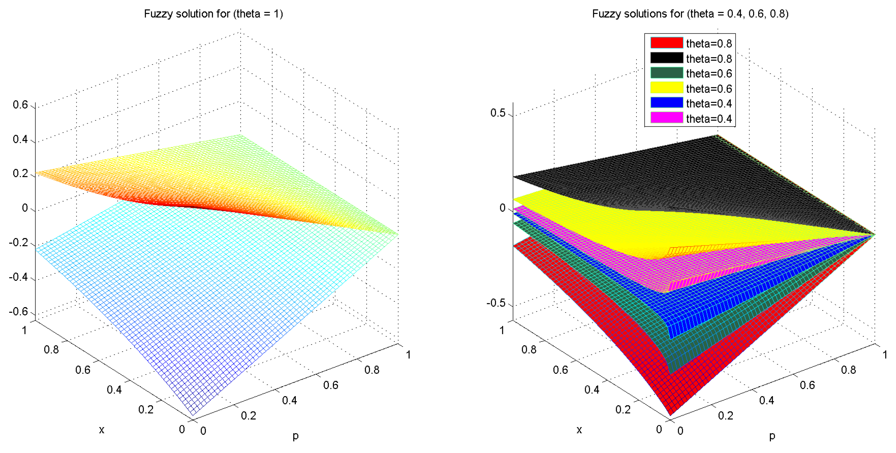
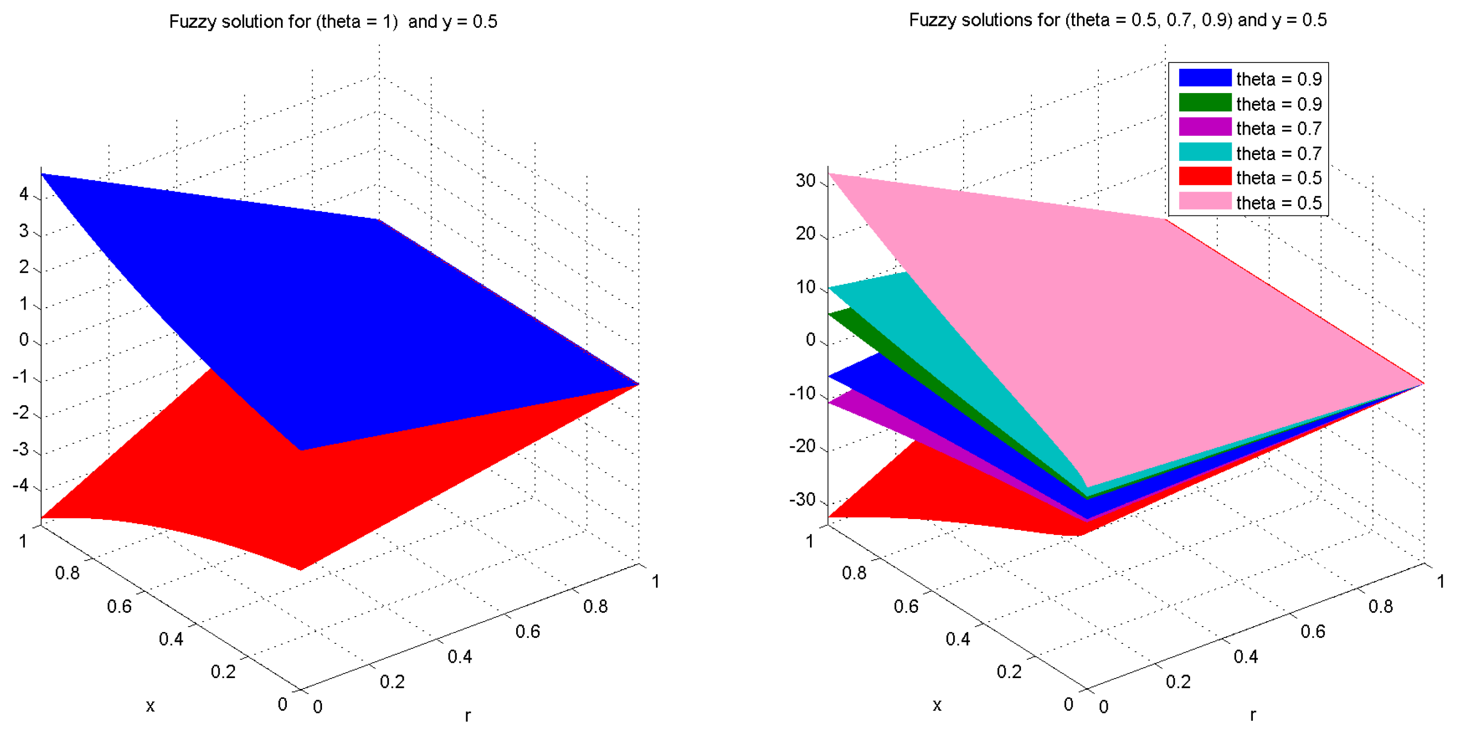
4. Some Numerical Examples

Now, we discuss numerical examples for the useability and authenticity of established results. For the solutions of numerical problems, we apply a conformable double Laplace transform. In this section, we also provide 3D plots of solutions of numerical examples (See Figure 1, Figure 2, Figure 3 and Figure 4).
Example 1. 
We have the following FPDEs with 0 < θ 1 and k , l { i , i i }
D x y k , l θ u ( x , y ) = u ( x , y ) , u ( x , 0 ) = ϕ 1 ( x ) = γ e x , 0 x x 0 , u ( 0 , y ) = ϕ 2 ( y ) = γ e y , 0 y y 0 .
Since γ is a fuzzy number and ϕ 1 ( x ) and ϕ 2 ( y ) are [ i g H ] C differentiable then for k = l = i by Theorem 1 the problem (16) has a unique solution in C ( i , i ) ( Y , F R ) where Y = [ 0 , x 0 ] × [ 0 , y 0 ] .
Apply conformable double Laplace transform.
p s u ( s , p ) = s u ( s , 0 ) + p u ( 0 , p ) u ( 0 , 0 ) + u ( s , p ) , u ( s , 0 ) = γ s 1 , u ( 0 , p ) = γ p 1 .
Using initial conditions one can get
u ( s , p ) = γ s ( p s 1 ) ( s 1 ) + γ p ( p s 1 ) ( p 1 ) γ p s 1 = γ ( p 1 ) ( s 1 ) .
Apply inverse conformable double Laplace transform to obtain the solution
u ( x , y ) = γ e x θ θ + y θ θ .
Since ϕ 1 and ϕ 2 are not [ i i g H ] C differentiable, the rest of the cases do not have solutions.
Example 2. 
Let the following FPDEs with 0 < θ 1 , and k , l { i , i i }
D x y k , l θ u ( x , y ) = u ( x , y ) , u ( x , 0 ) = ϕ 1 ( x ) = γ e x , 0 x x 0 , u ( 0 , y ) = ϕ 2 ( y ) = γ e y , 0 y y 0 .
Since γ is a fuzzy number and ϕ 1 ( x ) and ϕ 2 ( y ) are [ i i g H ] C differentiable then for k = l = i i by Theorem 1 the Problem (17) has a unique solution in C ( i i , i i ) ( Y , F R ) where Y = [ 0 , x 0 ] × [ 0 , y 0 ] .
Apply conformable double Laplace transform
p s u ( s , p ) = s u ( s , 0 ) + p u ( 0 , p ) u ( 0 , 0 ) + u ( s , p ) , u ( s , 0 ) = γ s + 1 , u ( 0 , p ) = γ p + 1 .
Using initial conditions and rearranging one can get
u ( s , p ) = γ s ( p s 1 ) ( s + 1 ) + γ p ( p s 1 ) ( p + 1 ) γ p s 1 , = γ ( p + 1 ) ( s + 1 ) .
Apply inverse conformable double Laplace transform and the required solution is obtained as
u ( x , y ) = γ e x θ θ y θ θ .
Since ϕ 1 and ϕ 2 are not [ i g H ] C differentiable, the rest of the cases do not have solutions.
Example 3. 
We have the following FPDEs with 0 < θ 1 , and k , l { i , i i }
3 D x y k , l θ u ( x , y ) = D x k θ u ( x , y ) + D y l θ u ( x , y ) u ( x , y ) , u ( x , 0 ) = ϕ 1 ( x ) = γ e x , 0 x x 0 , u ( 0 , y ) = ϕ 2 ( y ) = γ e y , 0 y y 0 .
Since γ is a fuzzy number and ϕ 1 ( x ) and ϕ 2 ( y ) are [ i g H ] C differentiable, then for k = l = i by Theorem 1 the problem (19) has a unique solution in C ( i , i ) ( Y , F R ) where Y = [ 0 , x 0 ] × [ 0 , y 0 ] . Apply conformable double Laplace transform
( p s s p + 1 ) u ( s , p ) = ( s 1 ) u ( s , 0 ) + ( p 1 ) u ( 0 , p ) u ( 0 , 0 ) , u ( s , 0 ) = γ s 1 , u ( 0 , p ) = γ p 1 .
Using initial conditions and rearranging one can get
u ( s , p ) = γ ( p 1 ) ( s 1 )
Apply inverse conformable double Laplace transform the required solution is obtained as
u ( x , y ) = γ e x θ θ + y θ θ .
Example 4. 
We have the following FPDEs with 0 < θ 1 , and k , l { i , i i }
D x y k , l θ u ( x , y ) = u ( x , y ) y , u ( x , 0 ) = ϕ 1 ( x ) = γ e x , 0 x x 0 , u ( 0 , y ) = ϕ 2 ( y ) = y + γ e y , 0 y y 0 .
Since γ is a fuzzy number and ϕ 1 ( x ) and ϕ 2 ( y ) are [ i g H ] C differentiable then for k = l = i by Theorem 1 the problem (20) has a unique solution in C ( i , i ) ( Y , F R ) where Y = [ 0 , x 0 ] × [ 0 , y 0 ] . Apply conformable double Laplace transform
p s u ( s , p ) = s u ( s , 0 ) + p u ( 0 , p ) u ( 0 , 0 ) + u ( s , p ) 1 p 2 , u ( s , 0 ) = γ s 1 , u ( 0 , p ) = 1 p 2 + γ p 1 .
Using initial conditions and rearranging one can get
u ( s , p ) = γ s ( p s 1 ) ( s 1 ) + γ p ( p s 1 ) ( p 1 ) γ p s 1 + 1 p ( p s 1 ) 1 s p 2 ( p s 1 ) , = γ ( p 1 ) ( s 1 ) + 1 s p 2 .
Apply inverse conformable double Laplace transform the required solution is obtained as
u ( x , y ) = γ e x θ θ + y θ θ + y θ θ .
Example 5. 
We have the following FPDEs with 0 < θ 1 , and k , l { i , i i }
D x y k , l θ u ( x , y ) = u ( x , y ) + 4 x y + x 2 y 2 , u ( x , 0 ) = ϕ 1 ( x ) = γ e x , 0 x x 0 , u ( 0 , y ) = ϕ 2 ( y ) = γ e y , 0 y y 0 .
Since γ is a fuzzy number and ϕ 1 ( x ) and ϕ 2 ( y ) are [ i g H ] C differentiable then for k = l = i by Theorem 1 the problem (21) has a unique solution in C ( i , i ) ( Y , F R ) where Y = [ 0 , x 0 ] × [ 0 , y 0 ] . Apply conformable double Laplace transform
p s u ( s , p ) = s u ( s , 0 ) + p u ( 0 , p ) u ( 0 , 0 ) + u ( s , p ) + 4 s 2 p 2 4 s 3 p 3 , u ( s , 0 ) = γ s 1 , u ( 0 , p ) = γ p 1 .
Using initial conditions and rearranging one can get
u ( s , p ) = γ s ( p s 1 ) ( s 1 ) + γ p ( p s 1 ) ( p 1 ) γ p s 1 + 4 s 2 p 2 ( p s 1 ) 4 s 3 p 3 ( p s 1 ) , = γ ( p 1 ) ( s 1 ) + 4 s 3 p 3 .
Apply inverse conformable double Laplace transform the required solution is obtain as
u ( x , y ) = γ e x θ θ + y θ θ + x 2 θ y 2 θ θ 2 .

5. Applications of Fractional Fuzzy Goursat Problems

Fractional calculus is the generalization of usual calculus. In this section, we discuss some facts about the generalization of fractional differentiability and fractional transform. Let us consider the following fuzzy partial differential equation
D x y k , l θ u ( x , y ) = u ( x , y ) , k , l { i , i i } u ( x , 0 ) = ϕ 1 ( x ) = γ x θ θ , 0 x x 0 , u ( 0 , y ) = ϕ 2 ( y ) = γ sin ω y θ θ , 0 y y 0 .
Since γ is a fuzzy number and ϕ 1 ( x ) and ϕ 2 ( y ) are [ i g H ] C differentiable then for k = l = i by Theorem 1 the problem (22) has a unique solution in C ( i , i ) ( Y , F R ) where Y = [ 0 , x 0 ] × [ 0 , y 0 ] .
Now, apply conformable double Laplace transform
p s u ( s , p ) = s u ( s , 0 ) + p u ( 0 , p ) u ( 0 , 0 ) + u ( s , p ) , u ( s , 0 ) = γ s 2 , u ( 0 , p ) = γ ω ω 2 + p 2 .
Using initial conditions and rearranging Equation (23), one can get
u ( s , p ) = γ s ( p s 1 ) + γ p ω ( p s 1 ) ( ω 2 + p 2 ) γ s ( p s 1 ) , = γ p ω ( p s 1 ) ( ω 2 + p 2 ) .
By applying the inverse conformable double Laplace transform the required solution is obtain as
u ( x , y ) = γ ω e ( x y ) θ θ 2 cos ( ω y θ θ ) .
Note that the fractional transform discussed in this work, particularly in this problem, is more easy than the usual Laplace transform. Also, fractional differential equations and their solutions are generalizations of usual differential equations because if θ = 1 then, we obtain the usual form discussed in [13]. Moreover, the fractional partial differential Equation (22) and their solution produce the partial fractional differential equations and solutions for any value 0 < θ 1 , particularly if θ = 1 2 and ω = 1 then Equation (22) produce the following problem
D x y i , i 1 2 u ( x , y ) = u ( x , y ) , u ( x , 0 ) = ϕ 1 ( x ) = 2 γ x , if 0 x < , u ( 0 , y ) = ϕ 2 ( y ) = γ sin ( 2 y ) , if 0 y π 2 4 .
where solution of Equation (24) is u ( x , y ) = γ e 4 x y cos ( 2 y ) . Caputo’s fractional derivative of order 1 2 and first-order usual derivative of ϕ 1 ( x ) are the following, respectively,
D i 1 2 ϕ 1 ( x ) = D i 1 2 ( 2 γ x ) = γ and D i ( ϕ 1 ( x ) ) = 2 γ D i x = γ x
Caputo’s fractional derivative of ϕ 1 ( x ) and ϕ 2 ( y ) exist at 0 but the usual derivative does not exist at 0; therefore, the fractional derivative is the generalization of the usual derivative. Concluding the above facts, we claim that this work is more advanced than [13].

6. Conclusions and Future Direction

In this manuscript, we discussed fractional order fuzzy Goursat problems with Caputo’s gH-differentiability. The Goursat problems have partial differential equations with second-order mixed derivatives. Also, Caputo’s gH-differentiability has two types, [ i g H ] C differentiability and [ i i g H ] C differentiability. To avoid the difficulties of mixed derivative terms and two types of Caputo’s gH-differentiability, we convert the Goursat problem to four equivalent systems of fuzzy fractional integral equations. The four systems of fuzzy fractional integral equations produced for a Goursat problem due to two types the Caputo’s gH-differentiability. In this study, we discussed that all the equivalent systems of fuzzy fractional integral equations satisfy the FPDEs and boundary conditions of the Goursat problem. After that, we discussed the existence and uniqueness result of fuzzy Goursat problems by using equivalent systems of fuzzy fractional integral equations. In addition to theoretical proofs, we provided numerical examples to show the useability of the theoretical work. We used conformable double Laplace transform for the solutions of numerical examples. In the application, we discussed the generalization of PFDEs and the advantage of fractional differentiability over the usual differentiability. Moreover, we show the advantage of fractional transform over the usual Laplace transform. This manuscript presents 3D fuzzy plots of solutions to illustrate our findings. This type of setting is also interesting for other second-order fractional FPDEs like advection equations, advection-diffusion equations, heat equations, etc. Moreover, this study is also interesting with other types of fuzzy differences and differentiability. The stability analysis of the solutions of Goursat problems and other second-order fractional FPDEs with this type of setting is also interesting for study in the future.

Author Contributions

Conceptualization, N.J.; Validation, T.S.; Formal analysis, C.P. and T.S.; Investigation, C.P.; Writing—original draft, N.J.; Writing—review and editing, M.S.; Visualization, K.A.; Supervision, M.S. and K.A.; Funding acquisition, C.P. and T.S. All authors have read and agreed to the published version of the manuscript.

Funding

This research was funded by the National Science, Research and Innovation Fund (NSRF), and King Mongkut’s University of Technology North Bangkok with Contract no. KMUTNB-FF-67-B-31.

Data Availability Statement

Data sharing is not applicable to this article as no data sets are generated or analyzed during the current study.

Acknowledgments

The authors would like to thank the Prince Sultan University for the support of this work through TAS LAB.

Conflicts of Interest

The authors declare that they have no competing interests.

References

  1. Zadeh, L.A. Fuzzy sets. Inf. Control 1965, 8, 338–353. [Google Scholar] [CrossRef]
  2. Sori, A.A.; Ebrahimnejad, A.; Motameni, H. Elite artificial bees’ colony algorithm to solve robot’s fuzzy constrained routing problem. Comput. Intell. 2019, 36, 659–681. [Google Scholar] [CrossRef]
  3. Nasseri, S.H.; Ebrahimnejad, A.; Gholami, O. Fuzzy Stochastic Data Envelopment Analysis with Undesirable Outputs and its Application to Banking Industry. Int. J. Fuzzy Syst. 2017, 20, 534–548. [Google Scholar] [CrossRef]
  4. Xi, Y.; Ding, Y.; Cheng, Y.; Zhao, J.; Zhou, M.; Qin, S. Evaluation of the Medical Resource Allocation: Evidence from China. Healthcare 2023, 11, 829. [Google Scholar] [CrossRef]
  5. Jan, N.; Gwak, J.; Pamucar, D. A Robust Hybrid Decision Making Model for Human-Computer Interaction in the Environment of Bipolar Complex Picture Fuzzy Soft Sets. Inf. Sci. 2023, 645, 119163. [Google Scholar] [CrossRef]
  6. Jamal, N.; Sarwar, M.; Hussain, S. Existence criteria for the unique solution of first order linear fuzzy differential equations on the space of linearly correlated fuzzy numbers. Fractals 2022, 8, 2240221. [Google Scholar] [CrossRef]
  7. Jamal, N.; Sarwar, M.; Mlaiki, N.; Aloqaily, A. Solution of linear correlated fuzzy differential equations in the linear correlated fuzzy spaces. AIMS Math. 2023, 9, 2695–2721. [Google Scholar] [CrossRef]
  8. Buckley, J.J.; Feuring, T. Introduction to fuzzy partial differential equations. Fuzzy Sets Syst. 1999, 105, 241–248. [Google Scholar] [CrossRef]
  9. Allahviranloo, T.; Gouyandeh, Z.; Armand, A.; Hasanoglu, A. On fuzzy solutions for heat equation based on generalized Hukuhara differentiability. Fuzzy Sets Syst. 2015, 265, 1–23. [Google Scholar] [CrossRef]
  10. Zureigat, H.; Tashtoush, M.A.; Jassar, A.F.A.; Az-Zo’bi, E.A.; Alomari, M.W. A Solution of the Complex Fuzzy Heat Equation in Terms of Complex Dirichlet Conditions Using a Modified Crank–Nicolson Method. Adv. Math. Phy. 2023, 2023, 6505227. [Google Scholar] [CrossRef]
  11. Datta, D. An algorithm for solving fuzzy advection diffusion equation and its application to transport of radon from soil into buildings. Int. J. Syst. Assur. Eng. Manag. 2014, 8, 2129–2136. [Google Scholar]
  12. Jamal, N.; Sarwar, M.; Agarwal, P.; Mlaiki, N.; Aloqaily, A. Solutions of fuzzy advection-diffusion and heat equations by natural adomian decomposition method. Sci. Rep. 2023, 13, 18565. [Google Scholar] [CrossRef] [PubMed]
  13. Khastana, A.; Rodriguez-Lopezb, R. An existence and uniqueness result for fuzzy Goursat partial differential equation. Fuzzy Sets Syst. 2019, 375, 141–160. [Google Scholar] [CrossRef]
  14. Salahshour, S.; Allahviranloo, T.; Abbasbandy, S.; Baleanu, D. Existence and uniqueness results for fractional differential equations with uncertainty. Adv. Diff. Eq. 2012, 2012, 112. [Google Scholar] [CrossRef]
  15. Hoa, N.V. Fuzzy fractional functional differential equations under Caputo gH-differentiability. Commun. Nonlinear Sci. Numer. Simul. 2015, 22, 1134–1157. [Google Scholar] [CrossRef]
  16. Shah, K.; Seadawy, A.R.; Arfan, M. Evaluation of one dimensional fuzzy fractional partial differential equations. Alex. Eng. J. 2020, 59, 3347–3353. [Google Scholar] [CrossRef]
  17. Kumar, S.; Nisar, K.S.; Kumar, R.; Cattani, C.; Samet, B. A new Rabotnov fractional exponential function based fractional derivative for diffusion equation under external force. Mathe. Methods. Appl. Sci. 2020, 43, 4460–4471. [Google Scholar] [CrossRef]
  18. Arfan, M.; Shah, K.; Ullah, A.; Abdeljawad, T. Study of fuzzy fractional order diffusion problem under the Mittag-Leffler Kernel Law. Phys. Scr. 2021, 96, 074002. [Google Scholar] [CrossRef]
  19. Ahmad, N.; Ullah, A.; Ullah, A.; Ahmad, S.; Shah, K.; Ahmad, I. On analysis of the fuzzy fractional order Volterra-Fredholm integro-differential equation. Alex. Eng. J. 2021, 60, 1827–1838. [Google Scholar] [CrossRef]
  20. Khan, H.; Gomez-Aguilar, J.F.; Abdeljawad, T.; Khan, A. Existence results and stability criteria for ABC-fuzzy-Volterra integro-differential equation. Fractals 2020, 28, 2040048. [Google Scholar] [CrossRef]
  21. Khan, W.A.; Zarin, R.; Zeb, A.; Khan, Y.; Khan, A. Navigating Food Allergy Dynamics via a Novel Fractional Mathematical Model for Antacid-Induced Allergies. J. Math. Tech. Model. 2024, 1, 25–51. [Google Scholar]
  22. Khan, F.M.; Khan, Z.U. Numerical Analysis of Fractional Order Drinking Mathematical Model. J. Math. Tech. Model. 2024, 1, 11–24. [Google Scholar]
  23. Courant, R.; Hilbert, D. Methods of Mathematical Physics; Wiley: New York, NY, USA, 1989. [Google Scholar]
  24. Wazwaz, A.M. The variational iteration method for a reliable treatment of the linear and the nonlinear Goursat problem. Appl. Math. Comput. 2007, 193, 455–462. [Google Scholar] [CrossRef]
  25. Ahmad, J.; Mushtaq, M. Exact Solution of Linear and Non-linear Goursat Problems. J. Comput. Math. 2015, 3, 14–17. [Google Scholar] [CrossRef]
  26. Iftikhar, A.; Arif, W.; Zaman, L.; Naseem, T. Novel Techniques for Solving Goursat Partial Differential Equations in the Linear and Nonlinear Regime. IJEMD-M 2022, 1, 17–37. [Google Scholar]
  27. Bede, B. Mathematics of Fuzzy Sets and Fuzzy Logic; Springer: London, UK, 2013. [Google Scholar]
  28. Diamond, P.; Kloeden, P. Metric Spaces of Fuzzy Sets; World Scientific: Singapore, 1994. [Google Scholar]
  29. Bede, B.; Gal, S.G. Generalization of the differentiability of fuzzy-number-valued functions with applications to fuzzy differential equation. Fuzzy Sets Syts. 2005, 151, 581–599. [Google Scholar] [CrossRef]
  30. Bahrami, F.; Alikhani, R.; Khastan, A. Transport equation with fuzzy data. Iran. J. Fuzzy Syst. 2018, 15, 67–78. [Google Scholar]
  31. Erdélyied, A. Higher Transcendental Functions; McGraw-Hill: New York, NY, USA, 1955; Volume 1. [Google Scholar]
  32. Rahman, N.A.A.; Ahmad, M.Z. Solving fuzzy fractional differential equations using fuzzy Sumudu transform. J. Nonlinear Sci. Appl. 2017, 10, 2620–2632. [Google Scholar] [CrossRef]
  33. Özkan, O.; Kurt, A. Exact Solution of Fractional Partial Differential Equation Systems with Conformable Derivative. Filomat 2019, 33, 1313–1322. [Google Scholar] [CrossRef]
Figure 1. 3D plots of the solution of Example (1) with θ = 1 , 0.9 , 0.8 , 0.7 , 0.6 .
Fractalfract 08 00250 g001
Figure 2. 3D plots of the solution of Example (2) with θ = 1 , 0.8 , 0.6 , 0.4 .
Fractalfract 08 00250 g002
Figure 3. 3D plots of the solution of Example (4) with θ = 1 , 0.9 , 0.7 , 0.6 .
Fractalfract 08 00250 g003
Figure 4. 3D plots of the solution of Example (5) with θ = 1 , 0.9 , 0.7 , 0.5 .
Fractalfract 08 00250 g004
Disclaimer/Publisher’s Note: The statements, opinions and data contained in all publications are solely those of the individual author(s) and contributor(s) and not of MDPI and/or the editor(s). MDPI and/or the editor(s) disclaim responsibility for any injury to people or property resulting from any ideas, methods, instructions or products referred to in the content.

