Physical Modeling of a Water Hydraulic Proportional Cartridge Valve for a Digital Twin in a Hydraulic Press Machine

Abstract

Digital twins are an emerging technology that can be harnessed for the digitalization of the industry. Steel industry systems contain a large number of electro-hydraulic components as proportional valves. An input–output model for a water proportional cartridge valve was derived from physical modeling based on fluid mechanics, dynamics, and electrical principles. The valve is a two-stage valve with two two/two-way water proportional valves as the pilot stage and a marginally stable poppet-type cartridge valve as the main valve. To our knowledge, this is the first time that an input–output model was derived for a two-stage proportional cartridge valve with a marginally stable main valve. The orifice equation, which is based on Bernoulli principles, was approximated by a polynomial, which made the parameter estimation easier and modeling possible without measuring the pressure of the varying control volume, in contrast with previous studies of similar types of valves situated in the pilot stage part of the valve. This work complements previous studies of similar types of valves in two ways: (1) data were collected when the valve was operating in a closed loop and (2) data were collected when the valve was part of a press mill machine in a steel manufacturing plant. Model parameters were identified from data from these operating conditions. The parameters of the input–output model were estimated by convex optimization with physical constraints to overcome the problems caused by poor system excitation. For comparison, a simple linear model was derived and the least squares method was used for the parameter estimation. A thorough estimation of the parameters’ relative errors is presented. The model contains five parameters related to the design parameters of the valve. The modeled position output was in good agreement with experimental data for the training and test data. The model can be used for the real-time monitoring of the valve’s status by the model parameters. One of the model parameters varied linearly with the production cycles. Thus, the aging of the valve can be monitored.

1. Introduction

A digital twin is a virtual representation of a physical entity. It aims to be the digital mirror of a system’s behavior by accounting for condition monitoring, allowing for its control, and creating predictions of its behavior. It is also one of the enablers of Industry 4.0. We can find different definitions in the literature, but this concept was introduced in 2003 [1]. According to a narrower definition [2], a digital twin has the following characteristics: it is a model of a physical object that exists, it is associated with a data set that evolves and grows with time, the parameters of the model are updated continuously from the data, and it can render predictions with a high enough level of accuracy and confidence for application. Furthermore, according to this definition, the model should be a physics-based type of model. Therefore, digital twins of mechatronic devices, where sensors collect data that are sent to their virtual mirror and actuators allow one to control the system’s behavior, play an essential role in the digitalization of the industry [3,4]. In this study, we formulated a digital twin of a valve that fits the definition in [2]. Such digital twins have the advantage of being interpretable for engineers who work with certain specific applications [5].

Digital twins can be used for modeling various technical systems in the steel industry. Feng Xiang described how to apply digital twins when considering data over the entire life cycle of a product [6]. Karandaev et al. (2021) developed a digital twin for the purpose of mirroring and controlling metal behavior in wire-rolling processes [7]. Gasiyarova et al. (2021) developed an observer of angular gaps in a rolling stand’s mechanical transmission, where this observer contained information about the transmission’s failure, which was achieved by considering the algorithm’s computational cost for real-time monitoring [8]. A comparison of some types of behavioral models used for digital twins of a ring-rolling machine was investigated in Bautista and Rönnow (2023); specifically, autoregressive with exogenous variables (ARX), autoregressive moving average with exogenous variables (ARMAX), and orthonormal basis function (OBF) models were investigated [9]. OBF-ARX and OBF-ARMAX were used for digital twins of the various subsystems of a ring-rolling machine in [10].

Hydraulic valves are used in hydraulic control systems for the modulation and control of the position, speed, or force of actuators. They provide the interface between the power elements, which are generally pumps, and the actuators, which are usually hydraulic cylinders. A more detailed description of hydraulic valves and its classification can be found in [11]. Electro-hydraulic proportional/servo valves have certain disadvantages compared with high-speed on/off valves, such as a complex structure and high power losses. Research on high-speed valves is currently being carried out because of their fast response. However, the flow capabilities of high-speed on/off valves are insufficient for applications with large flow requirements. Two-stage proportional cartridge valves are used in such applications. Two-stage proportional cartridge valves with a poppet-type construction, which give better sealing compared with the traditional large flow proportional cartridge valve, have been succesfully used in large-flow, fast-response, and high-pressure applications [12,13].

Research on cartridge valves has been ongoing for the last two decades [14,15]. The energy required by a system to control the hydraulic cylinder position was reduced in Song Liu and Bin Yao (2002) through a particular combination of five proportional cartridge valves [16]. The same authors developed an adaptive robust control of the same hydraulic system by considering the valve manufacturer’s information about flow characteristics instead of identifying the flow model parameters with experimental data [17]. Then, they identified the flow mapping of the cartridge valve in different ways [18,19]. A reduction in the energy consumption was achieved by introducing an accumulator and designing a new controller [20]. A directional control valve with a three-stage structure based on two high-speed on/off solenoid valves as the pilot stage and two poppet-type cartridge valves as the secondary stage was proposed in [21] to get a fast response and maximize the flow and pressure. Daling Yue et al. (2021) proposed a control strategy based on optimizing the duty ratios of positive and negative pulse voltages to decrease the opening and closing times of a screw-in cartridge valve [22]. The same research group further developed optimizations in the opening and closing times of a valve by proposing a hybrid voltage control strategy in which a preload voltage and hold voltage stage were added to the positive pulse and negative pulse voltages [13]. A cartridge proportional valve, similar to the one under study in this work, was investigated in prior studies. In these studies, the medium used to transfer energy between the power element and the actuator was water, and the valves were used for large flows under high-pressure conditions, as was the case in our study. The analytical expressions of the behavior of an injection machine with non-linear flow forces under different poppet geometries of a cartridge valve were studied and validated by physical simulations using AMESim, thereby demonstrating that using the most optimal choice of parameters results in improved process performance [12]. An optimal design of a two-stage proportional cartridge valve with two two/two-way water hydraulic proportional valves as the pilot stage and a poppet-type cartridge valve as the main valve was proposed in [23]. An extensive physical model of the valve was also developed and implemented in Matlab/Simulink R2019a to simulate the dynamic behavior of the valve. A multi-objective optimization was carried out to obtain a desired step response of the valve. The flow force was obtained from CFD simulations after optimizing the dimensional parameters of the valve orifice to minimize the flow force. A prototype was developed and experimentally tested to validate the simulated dynamic simulations [23].

Hydraulic valves are dynamic systems; as such, they can be modeled by physics-based or behavioral models, in which the former are derived from the laws of physics, and the latter describe the relationship between input and output signals via, for example, artificial neural networks [24]. Junhui et al. proposed a proportional directional valve, and they described its dynamical behavior by a physics-based model [25]. A physics-based model for describing the non-linear valve flow of a proportional valve was developed for the robust control of its position [26]. Physics-based models were used to model and control the position of proportional directional valves [27]. A physics-based model was proposed for a proportional pressure-reducing valve and was formulated by considering the dead zone and hysteresis effects for pressure tracking with a robust control method [28]. Regarding poppet-type cartridge valves and a physics-based model, parameter identification was used to identify the valve flow mapping, as well as the valve flow rate [18,19,21]. Michele proposed a novel Hammerstein dynamical model for modeling a hydraulic actuation system; this model was constructed for the purpose of control, and the model was constructed using a neural network in the non-linear static part and an ARX model for the linear dynamical part [29]. Black box models were used for system identification in hydraulic directional control valves [30]. A large servo-valve-controlled hydraulic system’s pressure dynamics was modeled using neural network model structures [31].

In this study, we derive for the first time (to our knowledge) a model and identify the parameters of a water two-stage proportional cartridge valve for high-pressure hydraulics. The pilot stage had two 2/2-way water proportional valves, and the main valve is a marginally stable poppet-type cartridge valve. In contrast, previous studies of poppet-type cartridge valves used a stable configuration. Additionally, this work is based on identifying the model parameters rather than optimizing the design parameters [23]. We also approximate the orifice equation via a polynomial to make the parameter estimation easier, as well as to make modeling possible without a pressure sensor in the control volume (which is situated in the main stage, cf. [23]). The parameters related to the flow mappings and flow rate were estimated for several poppet-type cartridge valves [18,19,21] with data collected in the laboratory. This is the first identification of a system of two valves, i.e., the control valve and the main valve, where the main valve is a poppet-type cartridge valve. Moreover, the data used to estimate the model parameters were collected when the valve was part of a hydraulic press. It was operated as the plant in a closed-loop system. The hydraulic press machine, which is composed of more than 50 valves and 5 hydraulic cylinders, was situated in a steel manufacturing plant. Each hydraulic cylinder reaches pressures of up to $2.5\times {10}^7$ Pa during a production cycle. The proposed model is derived from physical modeling based on fluid mechanics, dynamics, and electrical principles. The model parameters are related to the design parameters of the valve, and the parameter estimation is sufficiently fast to update the model parameters between production cycles. The estimated parameters could be used for real-time monitoring of the valve’s status, as well as provide a diagnosis. The interpretation of the model parameters is relatively easy since we use a physical model. The model can be used as a digital twin, where the parameters are monitored to show the aging of the valve; this was seen in data from industrial production.

2. Device and Operation

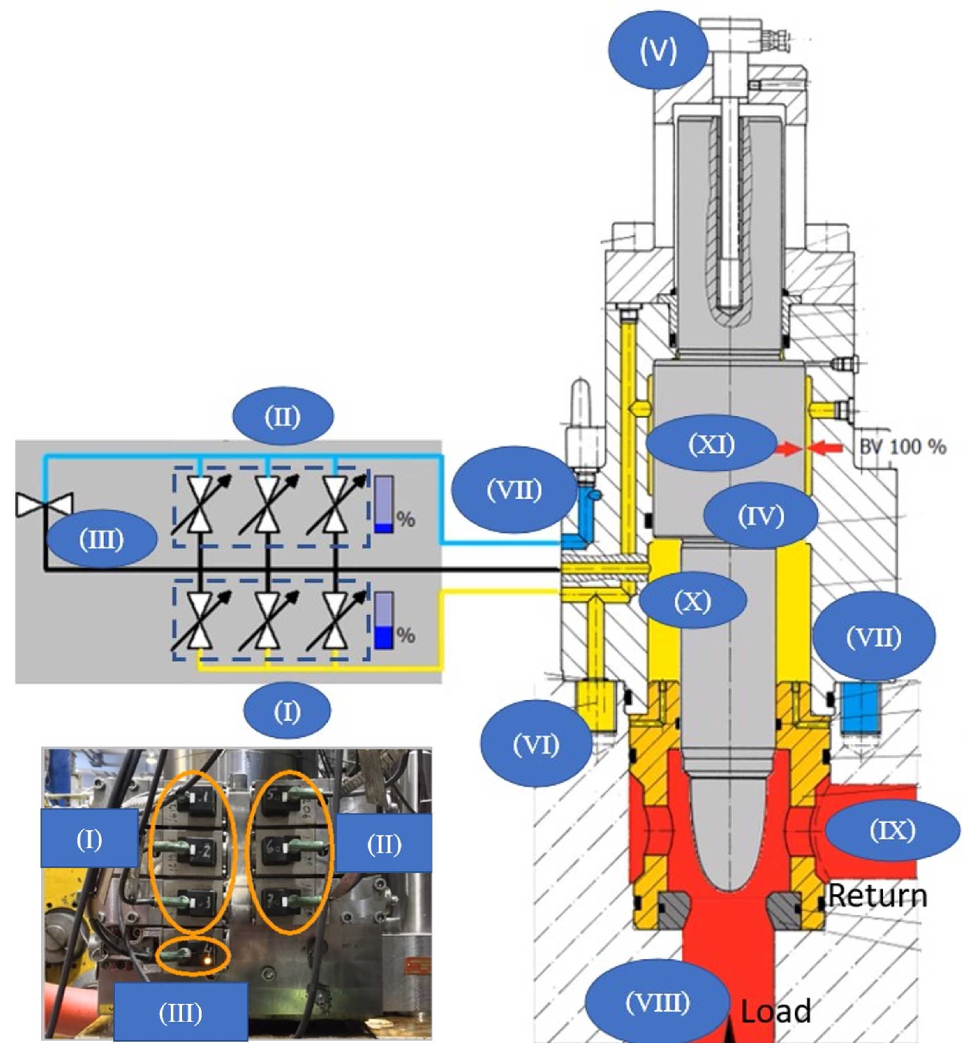
Figure 1 shows, in detail, the two-stage 2/2-way proportional cartridge valves under study. The pilot stage involve two groups of proportional spool valves: group (I) with three valves, and group (II) with another three. Each pilot valve is controlled by a solenoid, and they contain a pre-loaded spring attached. A similar type of pilot valves can be seen in detail in [23]. An emergency shut-down valve (III), a pilot-operated spindle (IV), an LDTV sensor (V), and two hydraulic circuits (one from (VI) to (VII), and another one from (VIII) to (IV), which represent the lower chamber (X) and the upper chamber (XI)) are included. Notice that there is no spring attached to the spindle (IV). More details about the spindle in similar valves and an emergency shut-down valve type that could be used for this application can be found in [23,32], respectively.

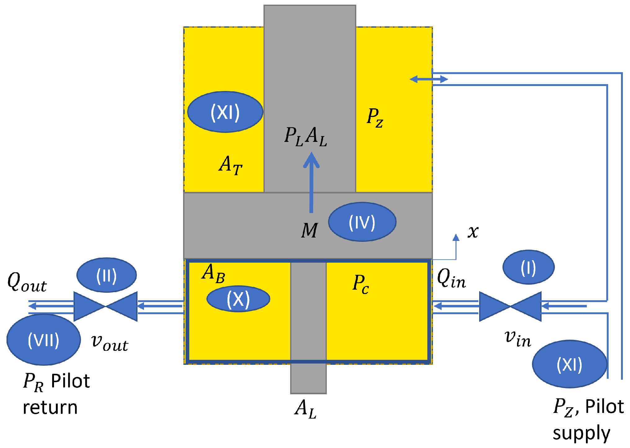
Figure 2 illustrates how the valve operates. There are certain differences, as can be seen from Figure 1. The three valves of group (I) in Figure 1 are represented by an equivalent single valve (I) in Figure 2. The valves (II) in Figure 1 are also represented by one equivalent valve (II) in Figure 2. There is a difference between the area of the upper part of the spindle, i.e., $A_T$, and the area of the lower part, i.e., $A_B$ (see Figure 2). Thus, the cross-sectional areas in contact with the fluid are different. $P_L{A}_L$ is the force exerted by the liquid going from (VIII) to (IX) to the spindle (IV).

To illustrate the valve’s behavior, we assumed the initial position of the spindle to be at its lowest position, which is to say that when the lower part of the spindle touches the bottom part of the container ($x=0$), the pilot valves are closed, i.e., $v_{in}\left(t\right)=v_{out}\left(t\right)=0$, $P_R=0$, $P_Z>0$, and $P_L{A}_L<P_Z{A}_T+Mg$. If $v_{in}>0$ and $v_{out}=0$, $Q_{in}>0$; then, $Q_{out}=0$, x increases, and fluid goes from (XI) to (VI). In contrast, if $v_{in}=0$ and $v_{out}>0$ when there is fluid in (X) and $P_L{A}_L<P_Z{A}_T$, then $Q_{in}=0$ and $Q_{out}>0$, which makes x decrease when the fluid went from (X) to (VII). In this study, the liquid that goes from (VI) to (VII), as well as from (VIII) to (IX), is 94% drinking water and 6% Hysol SL 36 XBB, respectively. Other additives that are used to harden the water and reduce the foam were Castrol Antifoam 101 and Castrol Antifoam S 105.

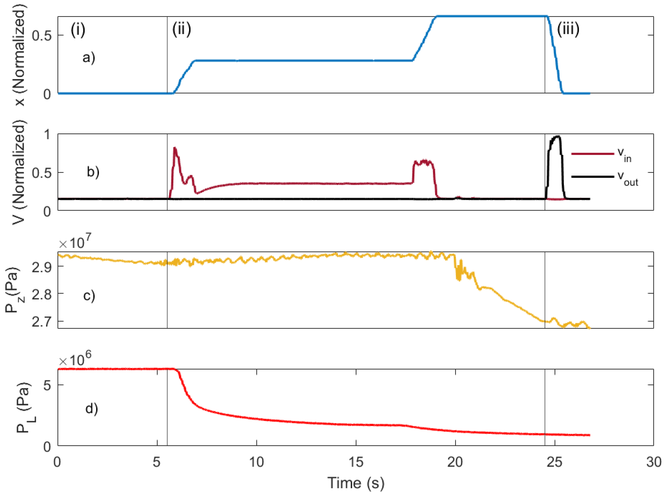
The operating conditions of the valve are determined by the fact that this is used for the production of steel tubes and the valve is the plant in a closed-loop system. The operating conditions can be split into (i), (ii), and (iii) (see Figure 3): (i) The initial conditions of the valve occurs when $x=0$ for the spindle (IV) of the main valve, when $v_{in}=v_{out}=0$ for the pilot valves (I) and (II), when the upper chamber of the main valve (XI) is full of water with $P_z\left(t\right)=3\times {10}^7$ Pa, and when $P_L\left(t\right)=0.6\times {10}^7$ Pa (see Figure 2 and Figure 3(i)). (ii) Once $v_{in}\left(t\right)>0$, then group (I) of the pilot valves let $Q_{in}>0$, and the spindle (IV) of the main valve starts to move such that $x\left(t\right)>0$; furthermore, $P_L\left(t\right)$ drops to $0.3\times {10}^7$ Pa in a few seconds (see Figure 3d). (iii) If $v_{in}\left(t\right)=0$ and $v_{out}\left(t\right)>0$, then the water from the lower chamber of the main valve (X) leaves the valve to the reservoir of group (II); hence, $x\left(t\right)$ decreases. This last step takes place when $P_L$ is approximately $0.1\times {10}^7$ Pa (see Figure 3d). It is noted that the value of $P_Z=2.9\times {10}^7$ Pa holds for most of the time but drops to $P_Z=2.7\times {10}^7$ Pa in the last third of the valve operation time; however, the spindle’s position x is not affected by it due to the ratio between $P_Z$ and $P_L$ (see Figure 3a,c). As a consequence of how the valve operates, x remains constant as long as $v_{in}\left(t\right)=v_{out}\left(t\right)=0$. However, this is not the case between $t=10$ s and $t=20$ s in (ii) due to the valve’s leakage (see Figure 3a,b). This last observation was discussed with the maintenance engineers.

The experimental data collected for this study were of the valve operating as the interface between a hydraulic pump and a single-rod linear actuator of one of the hydraulic control systems of a hydraulic press machine from a steel manufacturing plant. The signals from position x of the spindle (IV) and the voltages applied to the coils of the pilot valves (I) and (II) were $v_{in}\left(t\right)$ and $v_{out}\left(t\right)$, respectively. These signals are recorded by the data acquisition system IBA-DAQ with a sampling time of 0.03 s and an amplitude range of 0–1, where 0 corresponded to the minimum value and 1 to the maximum one. $v_{in}\left(t\right)$ and $v_{out}\left(t\right)$ are generated by a programmable logic computer with pulse-width-modulated signals of 24 V. The position of spindle $x\left(t\right)$ is controlled by a feedback control structure with a proportional–integral–derivative digital controller.

3. Modeling

This section is divided into three subsections: The first one describes the physical model of the valve; in the second, we describe the parameter estimation of the models; and in the last, the model validation is explained.

3.1. Physical Model

A physical model of the valve shown in Figure 1 and Figure 2 is presented in this section. It was based on the formulation detailed in Chapter 4 of [11], which uses conventional equations from fluid mechanics, dynamics, and electrical principles applied to hydraulic valves. In this work, the pressure in the upper chamber of the spindle (XI) $P_c\left(t\right)$ and the armature’s position of the pilot valves (I) and (II) were not measured; hence, we derived a model that connects the position x and the control signals $v_{in}\left(t\right)$ and $v_{out}\left(t\right)$ (see Figure 3a and b, respectively). These signals are given using a normalized scale. This section is divided based on the analysis of the valve as a system composed of different subsystems, as well as a system that is subject to different principles: the first part is the proportional pilot valves of both groups, i.e., (I) and (II); for the second, we have the volumetric flow rate of the pilot valves; next, a description of the the main valve’s control volume (X) is written; in the fourth part, the equation of motion for the spindle (IV) of the main valve is shown; then, an approximation of the $P_c$ in the main valve’s (X) is described in detail; and then lastly, in the sixth part, the input–output system model is shown. This input–output model implicitly describes all subsystems of the valve. The different parts can be classified according to its principles. The first part uses equations from dynamics and electrical principles. The second, third, and fourth parts describe conventional equations from fluid mechanics applied to the modeling of the valve shown in Figure 1 and Figure 2. The fourth part shows the second Newton’s law applied to the main valve’s spindle (IV) in Figure 1 and Figure 2. The last two parts give an approximation of $P_c$ and the input–output system model, respectively.

1.

Pilot valve model (I and II): These pilot valves consist of a solenoid, its armature, and a pre-loaded spring. Equations (3.6) and (3.7) in [11] describe a third-order coupled system, which, in this case, is the dynamics of the armature and the electrical circuit of the coil. We assume that the time constants of the armature’s motion are much smaller than those of the spindle’s motion. Therefore, we neglect the inductance of the coil’s circuit, the linear momentum, the viscous force, the flow forces acting on the armature, and the induced electromagnetic force from the armature’s motion. The last one is allowed because the electromagnetic force on the armature was greater; as such, we obtain

$$k{y}_i=\frac{\alpha v_{max}}{R}{v}_i-F_0$$

(1)

for valve i, where $i=\left\{1,\cdots ,m+l\right\}$. In this case, $m=l=3$ (see Figure 1). By setting $v_i=v_0$ for $y_i=0$ to derive $F_0$, we obtain

$$y_i\left({\overline{v}}_i\right)=\frac{\alpha v_{max}}{Rk}{\overline{v}}_i$$

(2)

where ${\overline{v}}_i=v_i-v_0$. ${\overline{v}}_i$ assumes $v_0$ as the offset of $v_i$, which is assumed to be the same for all pilot valves (see Figure 3b). All pilot valves are of the same type.

2.

Volumetric flow rate of the pilot valves (I and II): The standard Equation (4.1) in [11] is used to describe the flow (which assumed the fluid was incompressible with a high Reynolds number (i.e., laminar flow)). As such, we obtain

$$Q_i=c_{d}A\left({\overline{v}}_j\right)\sqrt{\frac{2}{\rho }\left(P_i\right)},$$

(3)

where $A_i\left({\overline{v}}_j\right)=w{y}_i\left({\overline{v}}_j\right)$ is the discharge flow area when assuming a rectangular section, which depends on the voltage applied to the coil of the pilot valve i. $P_i=(P_z-P_c)$ for $i=\left\{1,2,\cdots ,m\right\}$, and $P_i=P_c$ for $i=\left\{m+1,\cdots ,m+l\right\}$. We substitute j by subindexing $in$ for $i=\left\{1,2,\cdots ,m\right\}$, as well as by subindexing $out$ for $i=\left\{m+1,\cdots ,m+l\right\}$, i.e., $v_{in}$ and $v_{out}$ control $y_i$ for $i=\left\{1,\cdots ,m\right\}$ and $i=\left\{m+1,\cdots ,m+l\right\}$, respectively.

3.

The deformable volume (X) of the main valve is chosen as the control volume, as indicated by the solid blue line in Figure 2. The change in the control volume is understood as a function of the spindle’s position. For an incompressible fluid, the continuity Equation (5.5) in [33] becomes

$$A_B\dot{x}=Q_1+\cdots +Q_i+\cdots +Q_m-Q_{m+1}-\cdots -Q_{m+l}.$$

(4)

The flow of the pilot valves of group (I), i.e., $i=\left\{1,2,\cdots ,m\right\}$, increases the volume of the lower chamber (X), whereas the flow of those of group (II), i.e., $i=\left\{m+1,m+2,\cdots ,m+l\right\}$, decreases the same volume. The contribution of the assumption of water being incompressible to the modeling errors is analyzed in detail in Section 4.2.

4.

The spindle (IV) equation of motion of the main valve determines the motion of the main valve’s spindle, which is

$$M\ddot{x}+B\dot{x}=A_B{P}_c\left(t\right)-A_T{P}_z-F_{fm}sgn\left(\dot{x}\right)-F_{flow}+A_L{P}_L-Mg,$$

(5)

when ${\overline{v}}_{in}>0$ or ${\overline{v}}_{in}>0$. For a marginally stable valve, as with the one under study, there is no spring; hence, no term was proportional to x. $F_{flow}$ is the force exerted by the flow going from (VIII) to (IX) in Figure 1. An analysis of the flow forces allows for the term $A_L{P}_L$ to appear in the equation. $Mg$ is the force given by the main valve’s spindle mass. We assume that the Coulomb friction term can be neglected relative to $A_B{P}_c\left(t\right)$ and $A_T{P}_z$ due to a difference of 3–5 orders of magnitude when assuming friction between steel and rubber, i.e., the seal’s material. Furthermore, as we have values of $P_L\ll P_z$ (cf. scale of Figure 3c,d) and $A_L\ll A_T$ (cf. Figure 2), we thus obtaine $A_L{P}_L\ll A_T{P}_z$, as well as $Mg\ll A_T{P}_z$. The flow forces can be described by

$$F_{flow}=\rho L{K}_q\dot{x}+\rho L{K}_c{P}_L+K_{fq}(x-x_o)+K_{fc}(P_L-P_{L_o})$$

(6)

which can be obtained after deriving and linearizing with respect to x and $P_L$ (see Equation (4.20) in [11]). The subscript “o” signifies the nominal operating conditions of the valve. Considering the control volume, as illustrated in Figures 4–21 by dashed lines and the dimension given in Equation (4.122), both in [11], as well as the operating conditions of the hydraulic valve under study, we consider $F_{flow}$ to be negligible relative to $A_B{P}_c\left(t\right)$ and $A_T{P}_z$. This is because there is a difference of two orders of magnitude. More information about how to derive the expression of the coefficients in (6) can be found in Chapter 4, more specifically in Sections 4.3 and 4.6, in [11]. Finally, we obtain the main valve’s spindle equation of motion, which is

$$\left\{\begin{array}{cc}M\ddot{x}+B\dot{x}=A_B{P}_c\left(t\right)-A_T{P}_z\hfill & \mathrm{if}{\overline{v}}_{in}\mathrm{or}{\overline{v}}_{out}>0\hfill \\ \dot{x}=0,\hfill & \mathrm{if}{\overline{v}}_{in}={\overline{v}}_{out}=0\hfill \end{array}\right..$$

(7)

These equations are valid for $x\in [0,x_{max}]$. The case of ${\overline{v}}_{in}\left(t\right)={\overline{v}}_{out}\left(t\right)=0$ describes the system when $P_c\left(t\right)$ cannot be derived from Equations (3) and (4); see Equation (12).

5.

Approximation of $P_c$ in the main valve (X): Since $P_c$ is not measured, it is derived from Equations (3) and (4). Furthermore, knowing that the pilot valves are identical, and that ${\overline{v}}_{in}\left(t\right)$ is applied to all of the coils of pilot valves (I) and ${\overline{v}}_{out}\left(t\right)$ to (II) (see Figure 1 and Equation (4)), we obtain

$$A_B\dot{x}=m{Q}_{in}-n{Q}_{out},$$

(8)

where $Q_{in}=Q_1=\cdots =Q_m$ and $Q_{out}=Q_{m+1}=\cdots Q_{m+l}$. For $Q_{in}$, we use the auxiliary function

$$f_{in}\left(P_c\right)=\sqrt{(2/\rho )(P_Z-P_c)}$$

(9)

and for $Q_{out}$, we use

$$f_{out}\left(P_c\right)=\sqrt{(2/\rho )\left(P_c\right)},$$

(10)

which are derived from Equation (3). $f_{in}$ and $f_{out}$ are approximated by a Taylor series in $P_c$ around the operating point $P_c=P_{c,0}=\frac{A_T}{A_B}{P}_z$, which is the equilibrium point of Equation (7). By performing this, keeping the linear terms, and substituting these in Equation (8), we obtain

$$\begin{array}{cc}\hfill P_c\left(t\right)& =P_{c,0}+g({\overline{v}}_{in},{\overline{v}}_{out})\times \hfill \\ \hfill & (f_{in}(P_{c,0}{\overline{R}}_1{\overline{v}}_{in}\left(t\right)-f_{out}\left(P_{c,0}\right){\overline{R}}_2{\overline{v}}_{out}\left(t\right)-A_B\dot{x}),\hfill \end{array}$$

(11)

where

$$g({\overline{v}}_{in},{\overline{v}}_{out})=\frac{1}{f_{out}^{\prime }\left(P_{c,0}\right){\overline{R}}_2{\overline{v}}_{out}\left(t\right)-f_{in}^{\prime }\left(P_{c,0}\right){\overline{R}}_1{\overline{v}}_{in}\left(t\right)},$$

(12)

In the above, $f_{in}^{\prime }\left(P_{c,0}\right)$ is the first derivative of $f_{in}\left(P_c\right)$, which is evaluated at $P_{c,0}$; $f_{out}^{\prime }\left(P_{c,0}\right)$ is the first derivative of $f_{out}$; ${\overline{R}}_1=m{c}_d{w}_{in}\frac{{\alpha }_{in}{v}_{max}}{k_{in}{R}_{in}}$; and ${\overline{R}}_2=n{c}_d{w}_{out}\frac{{\alpha }_{out}{v}_{max}}{k_{out}{R}_{out}}$.

6.

The input–output system model is obtained by substituting Equation (11) into (7), where

$$\begin{array}{cc}\hfill M\ddot{x}& +B\dot{x}=A_{B}g({\overline{v}}_{in},{\overline{v}}_{out})\times \hfill \\ \hfill & (f_{in}\left(P_{c,0}\right){\overline{R}}_1{\overline{v}}_{in}\left(t\right)-f_{out}\left(P_{c,0}\right){\overline{R}}_2{\overline{v}}_{out}\left(t\right)-A_B\dot{x}).\hfill \end{array}$$

(13)

The auxiliary function $g({\overline{v}}_{in},{\overline{v}}_{out})$ is approximated by a Taylor series in ${\overline{v}}_{in}\left(t\right)$ and ${\overline{v}}_{out}\left(t\right)$ around ${\overline{v}}_{in,0}$ and ${\overline{v}}_{out,0}$, respectively, where ${\overline{v}}_{in,0}$, ${\overline{v}}_{out,0}\in \left(0,1\right]$. We keep the linear terms and Equation (13) is approximated by

$$\begin{array}{c}\hfill {\gamma }_1\ddot{x}+{\gamma }_2\dot{x}={\varphi }_1{\overline{v}}_{in}\left(t\right)+{\varphi }_2{\overline{v}}_{out}\left(t\right)+{\varphi }_3{\overline{v}}_{in}^2\left(t\right)+{\varphi }_4{\overline{v}}_{out}^2\left(t\right)+\cdots \\ \hfill \cdots +{\varphi }_5{\overline{v}}_{in}\left(t\right){\overline{v}}_{out}\left(t\right)+{\varphi }_6{\overline{v}}_{in}\left(t\right)\dot{x}+{\varphi }_7{\overline{v}}_{out}\left(t\right)\dot{x},\end{array}$$

(14)

where

$$\left\{\begin{array}{c}{\gamma }_1=\frac{M}{A_B}\ge 0\hfill \\ {\gamma }_2=\frac{B}{A_B}+\overline{g}{A}_B\ge 0\hfill \\ {\varphi }_1=\overline{g}{f}_{in}\left(P_{c,0}\right){\overline{R}}_1\ge 0\hfill \\ {\varphi }_2=-\overline{g}{f}_{out}\left(P_{c,0}\right){\overline{R}}_2\le 0\hfill \\ {\varphi }_3=g_{{\overline{v}}_{in}}^{\prime }({\overline{v}}_0,{\overline{v}}_0)f_{in}\left(P_{c,0}\right){\overline{R}}_1\le 0\hfill \\ {\varphi }_4=-g_{{\overline{v}}_{out}}^{\prime }({\overline{v}}_0,{\overline{v}}_0)f_{out}\left(P_{c,0}\right){\overline{R}}_2\ge 0\hfill \\ {\varphi }_5=g_{{\overline{v}}_{out}}^{\prime }({\overline{v}}_0,{\overline{v}}_0)f_{in}\left(P_{c,0}\right){\overline{R}}_1-g_{{\overline{v}}_{in}}^{\prime }({\overline{v}}_0,{\overline{v}}_0)f_{out}\left(P_{c,0}\right){\overline{R}}_2\in \mathcal{R}\hfill \\ {\varphi }_6=-g_{{\overline{v}}_{in}}^{\prime }({\overline{v}}_0,{\overline{v}}_0)A_B\ge 0\hfill \\ {\varphi }_7=-g_{{\overline{v}}_{out}}^{\prime }({\overline{v}}_0,{\overline{v}}_0)A_B\ge 0\hfill \end{array}\right.,$$

(15)

where $\overline{g}=g({\overline{v}}_0,{\overline{v}}_0)-g_{{\overline{v}}_{in}}^{\prime }({\overline{v}}_0,{\overline{v}}_0){\overline{v}}_0-g_{{\overline{v}}_{out}}^{\prime }({\overline{v}}_0,{\overline{v}}_0){\overline{v}}_0$, $g_{{\overline{v}}_{in}}^{\prime }({\overline{v}}_0,{\overline{v}}_0)$ is the derivative of $g({\overline{v}}_{in},{\overline{v}}_{out})$ with respect to ${\overline{v}}_{in}$, and $g_{{\overline{v}}_{out}}^{\prime }({\overline{v}}_0,{\overline{v}}_0)$ is the derivative of $g({\overline{v}}_{in},{\overline{v}}_{out})$ with respect to ${\overline{v}}_{out}$. Indeed, both are evaluated at ${\overline{v}}_{in}={\overline{v}}_{out}={\overline{v}}_0$. The sign of each of the parameters is specified explicitly in Equation (15), and this is performed in accordance with the physics of the device described in Equations (1)–(13). ${\varphi }_5$ is positive or negative depending on $A_T/A_B$. Notice that Equation (14) is a non-linear input–output model and linear in terms of the parameters. The non-linearities are related to ${\overline{v}}_{in}^2$, ${\overline{v}}_{out}^2$, ${\overline{v}}_{in}\dot{x}$, and ${\overline{v}}_{out}\dot{x}$. These terms are obtained from the square root in $\sqrt{\frac{2}{\rho }\left(P_i\right)}$ and the product $A\left({\overline{v}}_j\right)\times \sqrt{\frac{2}{\rho }\left(P_i\right)}$ in Equation (3).

3.2. Parameter Estimation

The parameters are estimated based on Equation (14). Equation (14) represents a non-linear system that relates the inputs ${\overline{v}}_{in}$ and ${\overline{v}}_{out}$ to the output x, and it is also linear in terms of the parameters. The data acquired by the DAQ were saved in a time-discrete form. Therefore, Equation (14) needs to be transformed to an equivalent time-discrete version. When the forward Euler method is used to discretize Equation (14), we obtain

$$\begin{array}{c}\hfill {\gamma }_1\frac{\dot{x}[n+1]-\dot{x}\left[n\right]}{T}+{\gamma }_2\frac{x[n+1]-x\left[n\right]}{T}={\varphi }_1{\overline{v}}_{in}\left[n\right]+{\varphi }_2{\overline{v}}_{out}\left[n\right]+{\varphi }_3{\overline{v}}_{in}^2\left[n\right]+\cdots \\ \hfill \cdots +{\varphi }_4{\overline{v}}_{out}^2\left[n\right]+{\varphi }_5{\overline{v}}_{in}\left[n\right]{\overline{v}}_{out}\left[n\right]+{\varphi }_6{\overline{v}}_{in}\left[n\right]\frac{x[n+1]-x\left[n\right]}{T}+{\varphi }_7{\overline{v}}_{out}\left[n\right]\frac{x[n+1]-x\left[n\right]}{T}.\end{array}$$

(16)

When $\dot{x}\left[n\right]=(x[n+1]-x\left[n\right])/T$ is applied and similarly for $\dot{x}[n+1]$ in Equation (16), we obtain

$$\begin{array}{c}\hfill \widehat{x}\left[n\right]=2x[n-1]-x[n-2]+{\theta }^{⊺}u\left[n\right]\end{array}$$

(17)

where x and $\widehat{x}$ are the experimental and model positions of the main valve’s spindle (IV), respectively [34].

$$\theta ={\left[\begin{array}{cccccccc}-\frac{{\gamma }_2{T}_s}{{\gamma }_1}& \frac{{\varphi }_1{T}^2}{{\gamma }_1{x}_{max}}& \frac{{\varphi }_2{T}^2}{{\gamma }_1{x}_{max}}& \frac{{\varphi }_3{T}^2}{{\gamma }_1{x}_{max}}& \frac{{\varphi }_4{T}^2}{{\gamma }_1{x}_{max}}& \frac{{\varphi }_5{T}^2}{{\gamma }_1{x}_{max}}& \frac{{\varphi }_6{T}_s}{{\gamma }_1}& \frac{{\varphi }_7{T}_s}{{\gamma }_1}\end{array}\right]}^{⊺}$$

(18)

and

$$u\left[n\right]=\left[\begin{array}{cc}& x[n-1]-x[n-2]\\ & {\overline{v}}_{in}[n-2]\\ & {\overline{v}}_{out}[n-2]\\ & {\overline{v}}_{in}^2[n-2]\\ & {\overline{v}}_{out}^2[n-2]\\ & {\overline{v}}_{in}[n-2]{\overline{v}}_{out}[n-2]\\ & {\overline{v}}_{in}[n-2](x[n-1]-x[n-2])\\ & {\overline{v}}_{out}[n-2](x[n-1]-x[n-2])\end{array}\right].$$

(19)

We formulate the parameter estimation problem as

$${\widehat{\theta }}_{LS}=argmi{n}_{\theta }\frac{1}{N}\sum _{n=1}^N\epsilon {[n;\theta ]}^2,$$

(20)

where $\epsilon [n;\theta ]=x\left[n\right]-\widehat{x}[n;\theta ]$, which gives an estimation of $\theta$ in Equation (17) by solving

$$\left(\sum _{n=1}^{N}u\left[n\right]u{\left[n\right]}^{⊺}\right){\widehat{\theta }}_{LS}=\sum _{n=1}^{N}u\left[n\right]\overline{x}\left[n\right]$$

(21)

as a system of linear equations, where $\overline{x}\left[n\right]=x\left[n\right]-2x[n-1]+x[n-2]$.

Alternatively, the problem of estimating the parameters in Equation (17) can be formulated by accordingly referring to Equation (4.1) in [35] as

$$\begin{array}{cc}\hfill & \underset{\theta \in {\mathcal{R}}^8}{min}\frac{1}{N}\sum _{n=1}^N\epsilon {[n;\theta ]}^2\hfill \\ \hfill & \mathrm{subject}\mathrm{to}\hfill \\ \hfill & \overline{\theta }\le 0\hfill \end{array}$$

(22)

where

$$\overline{\theta }={\left[\begin{array}{cccccccc}\theta \left(1\right)& -\theta \left(1\right)-1& -\theta \left(2\right)& \theta \left(3\right)& \theta \left(4\right)& -\theta \left(5\right)& -\theta \left(7\right)& -\theta \left(8\right)\end{array}\right]}^{⊺},$$

(23)

cf. Equation (18).

The parameter vector in Equation (23) is built from $\theta$ in Equation (18) and used in the mathematical optimization problem defined in Equation (22) to satisfy the standard form specified by Equation (4.1) in [35] and the physical constraints of the valve defined in Equation (15). $\overline{\theta }\left(1\right)=\theta \left(1\right)\le 0$ and $\overline{\theta }\left(2\right)=-\theta \left(1\right)-1\le 0$ are defined to obtain two poles in the discrete pole-zero map related to Equation (17), which is equivalent to a pole in the origin and a pole in the real left axis of the pole-zero map related to Equation (14). This is because ${\gamma }_1\ge 0$ and ${\gamma }_2\ge 0$ are such in Equation (15), and because there is no x term in Equation (14). Mathematical optimization problems with a quadratic objective function and affine constraints are known as quadratic programs (QPs), which comprise a convex optimization problem class. Therefore, the mathematical optimization problem defined in Equation (22) is a quadratic program (QP) and can be efficiently solved by iterative methods, like the interior point method [35]. To solve the optimization problem defined in Equation (22), we used CVX. CVX, which implements algorithms such as the interior point method to solve convex optimization problems, is a package for specifying and solving convex programs [36,37].

We used convex optimization to overcome problems caused by the closed-loop operation and the signals used in one production cycle. Thus, the excitation signals have a narrow band at low frequencies and a limited number of amplitudes. A system operating under feedback control is identifiable under specific conditions. For linear systems, if the feedback transfer function is persistently excited, then the system is identifiable (see Chapter 10 in [38]). The order of the controller and reference signal should be larger than that of the system, which was easily met in our case; furthermore, if the PID controller is of order two, then the system is of order five and the discrete time signal is of order ≥ 30.

3.3. Model Validation

The cross-validation was carried out with the data corresponding to a one-hour production after the production from which the data were used to estimate $\theta$ in Equation (17). We checked that the estimated values were in agreement with the physics of the valve described in Equation (15); in addition, we analyzed the residuals, i.e., $\epsilon [n;\widehat{\theta }]=x\left[n\right]-\widehat{x}[n;\widehat{\theta }]$. The mean squared error (MSE) indicator

$$MSE=\frac{1}{N}\sum _{n=1}^N{(x\left[n\right]-\widehat{x}[n;\widehat{\theta }])}^2$$

(24)

was computed, where N is the number of samples for the training or validation data sets. A dimensional analysis of the parameters of Equation (14), as described in Equation (15), was carried out, and the size of the estimated parameter values were checked to determine whether they were reasonable for the physical parameters described in Equation (15). We ended the model validation by computing the relative errors of the estimated parameters for different error sources [24].

4. Results and Discussion

This section is divided into three subsections: the first reports and analyzes the estimated parameters of the physical model; in the second, the relative errors of the estimated parameters for different error sources are computed and analyzed; and in the last section, the aging of the valve is analyzed over different production cycles.

4.1. Physical Model

Table 1. Estimated parameter values for the input–output system model in (17) and (18). ${\widehat{\theta }}_1$ and ${\widehat{\theta }}_2$ are least squares estimates, and ${\widehat{\theta }}_3$ was obtained by solving the mathematical optimization problem defined in Equation (22). $-1\le \theta \left(1\right)\le 0$, $\theta \left(2\right)\ge 0$, $\theta \left(3\right)\le 0$, $\theta \left(4\right)\le 0$, and $\theta \left(5\right)\ge 0$ are based on the physical constraints of the device.

$\mathit{\theta }$	Description	${\widehat{\mathit{\theta }}}_1$	${\widehat{\mathit{\theta }}}_2$	${\widehat{\mathit{\theta }}}_3$
$\theta \left(1\right)$	$-\frac{{\gamma }_2{T}_s}{{\gamma }_1}$	−1.16	−1.24	−0.99
$\theta \left(2\right)$	$\frac{{\varphi }_1{T}^2}{{\gamma }_1{x}_{max}}$	$1.01\times {10}^{-2}$	$7.04\times {10}^{-3}$	$1.01\times {10}^{-2}$
$\theta \left(3\right)$	$\frac{{\varphi }_2{T}^2}{{\gamma }_1{x}_{max}}$	$-4.34\times {10}^{-2}$	$-6.03\times {10}^{-2}$	$-5.61\times {10}^{-2}$
$\theta \left(4\right)$	$\frac{{\varphi }_3{T}^2}{{\gamma }_1{x}_{max}}$	-	$6.33\times {10}^{-2}$	-
$\theta \left(5\right)$	$\frac{{\varphi }_4{T}^2}{{\gamma }_1{x}_{max}}$	-	$3.37\times {10}^{-2}$	$2.78\times {10}^{-2}$
MSE training		$3.5\times {10}^{-5}$	$3.2\times {10}^{-5}$	$3.6\times {10}^{-5}$
MSE test		$3.8\times {10}^{-5}$	$3.8\times {10}^{-5}$	$4.5\times {10}^{-5}$

presents the results of the parameter estimation problem that were defined in Equations (20) and (22) in order to obtain the input–output system model described in Equation (17). We carried out three different parameter estimations. The first one was given by solving the standard least squares problem defined in Equation (20) with Equation (21). This provides

$$\begin{array}{c}{\widehat{\theta }}_1={\left(\begin{array}{ccc}\widehat{\theta }\left(1\right)& \widehat{\theta }\left(2\right)& \widehat{\theta }\left(3\right)\end{array}\right)}^{⊺},\end{array}$$

(25)

which estimated $\theta \left(1\right)$, $\theta \left(2\right)$, and $\theta \left(3\right)$ in Equation (18). Then, Equation (17) becomes

$${\widehat{x}}_1[n;{\widehat{\theta }}_1]=2x[n-1]-x[n-2]+{\widehat{\theta }}_1^{⊺}{u}_1\left[n\right]$$

(26)

with

$$\begin{array}{c}{u}_1\left[n\right]={\left(\begin{array}{ccc}u\left(1\right)& u\left(2\right)& u\left(3\right)\end{array}\right)}^{⊺},\end{array}$$

(27)

where $u\left(1\right)$, $u\left(2\right)$, and $u\left(3\right)$ are found in Equation (19). In the second case, ${\widehat{\theta }}_2$ is obtained by solving Equation (20) with Equation (21), as in the first case. The difference between the first and second cases is that, for the second case, we considered certain non-linear terms as having

$${\widehat{x}}_2[n;{\widehat{\theta }}_2]=2x[n-1]-x[n-2]+{\widehat{\theta }}_2^{⊺}{u}_2\left[n\right],$$

(28)

where

$$\begin{array}{c}{\widehat{\theta }}_2={\left(\begin{array}{ccccc}\widehat{\theta }\left(1\right)& \widehat{\theta }\left(2\right)& \widehat{\theta }\left(3\right)& \widehat{\theta }\left(4\right)& \widehat{\theta }\left(5\right)\end{array}\right)}^{⊺},\end{array}$$

(29)

and

$$\begin{array}{c}{u}_2\left[n\right]={\left(\begin{array}{ccccc}u\left(1\right)& u\left(2\right)& u\left(3\right)& u\left(4\right)& u\left(5\right)\end{array}\right)}^{⊺}.\end{array}$$

(30)

The third and last case correspond to solving Equation (22), which gave ${\widehat{\theta }}_3$. Then, Equation (17) becomes

$${\widehat{x}}_3[n;{\widehat{\theta }}_3]=2x[n-1]-x[n-2]+{\widehat{\theta }}_3^{⊺}{u}_3\left[n\right],$$

(31)

where

$$\begin{array}{c}{\widehat{\theta }}_3={\left(\begin{array}{cccc}\widehat{\theta }\left(1\right)& \widehat{\theta }\left(2\right)& \widehat{\theta }\left(3\right)& \widehat{\theta }\left(5\right)\end{array}\right)}^{⊺},\end{array}$$

(32)

and

$$\begin{array}{c}{u}_3\left[n\right]={\left(\begin{array}{cccc}u\left(1\right)& u\left(2\right)& u\left(3\right)& u\left(5\right)\end{array}\right)}^{⊺}.\end{array}$$

(33)

$\widehat{\theta }\left(4\right)$ and $\widehat{\theta }\left(8\right)$ are not considered in Equation (32) since their absolute values were $\le 1\times {10}^{-6}$ when solving Equations (22) and (23). $\widehat{\theta }\left(6\right)$, which is the parameter for the cross-term in ${\overline{v}}_{in}$ and ${\overline{v}}_{out}$, are ignored because during operation, ${\overline{v}}_{in}=0$ when ${\overline{v}}_{out}>0$ and ${\overline{v}}_{out}=0$ when ${\overline{v}}_{in}>0$; see Figure 3b. $\widehat{\theta }\left(7\right)$ is ignored because $u\left(7\right)$ is highly correlated with $u\left(1\right)$ and $u\left(2\right)$, and the MSE for the training and test data shown in Table 1 do not change when it is considered. We did not consider higher-order terms in Equations (14) and (15) because their absolute values were found to be $\le 1\times {10}^{-6}$ when solving the mathematical optimization problem defined in Equations (22) and (23).

In Table 1, the estimated parameter values obtained for the parameters defined in Equations (26), (28), and (31) are found. For ${\widehat{\theta }}_1$, we have no agreement between $\widehat{\theta }\left(1\right)$ and the physics of the system defined in Equation (15). From a systems theory perspective, this parameter value implies that the poles of (17) were $z=1$ and $z=-0.16$, where the last one relates to a pole with $f=16.67$ Hz, which is not possible when looking at Figure 3a,b. The $\widehat{\theta }\left(2\right)$ and $\widehat{\theta }\left(3\right)$ signs are in agreement with the physics; however, when assuming that both pilot valves (I) and (II) are equal to each other, there seems to be an anomaly in the valve. After a discussion with maintenance engineers at the manufacturing plant, a manual calibration of the springs in the pilot valves was performed after the maintenance of the valve. In ${\widehat{\theta }}_2$, the values of $\widehat{\theta }\left(1\right)$ and $\widehat{\theta }\left(4\right)$ are different in sign than the signs defined in Equation (15). Considering that the non-linear terms of the input–output model in Equation (28) increased the conditioning number of $\left({\sum }_{n=1}^N{\mathit{u}}_1\left[n\right]{\mathit{u}}_1{\left[n\right]}^{⊺}\right)$ by two orders of magnitude, this could be the reason we obtained these parameter values because of the poor excitation of the signals (see Figure 3a,b). ${\widehat{\theta }}_3$ gives values in agreement with the signs defined in (15) regarding the physics of the valve. As for ${\widehat{\theta }}_2$, there are differences between the second and third elements of the estimated parameter vector.

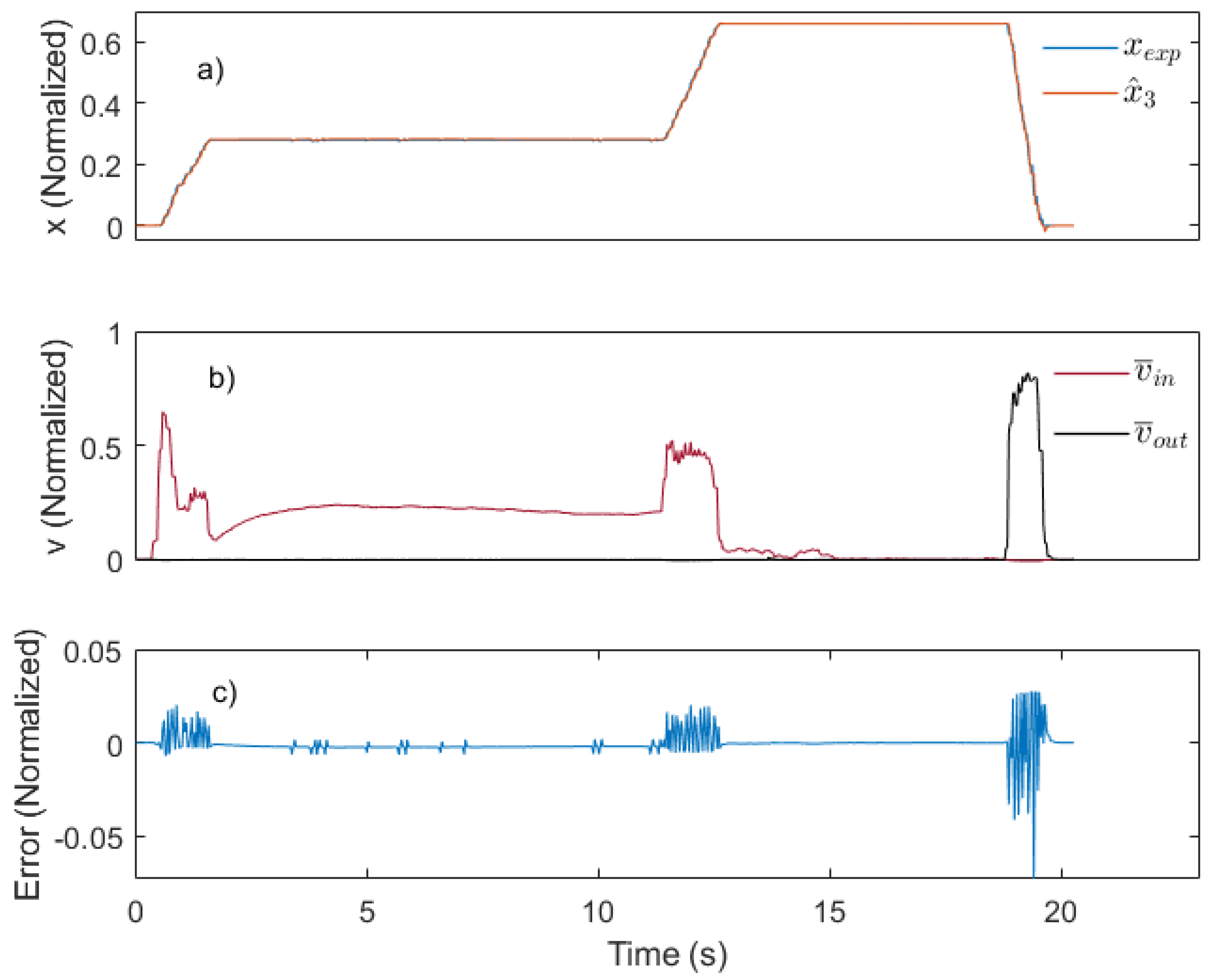
Figure 4a shows a comparison between $x\left[n\right]$ and ${\widehat{x}}_3\left[n\right]$, and this is achieved using validation data, i.e., signals from a different production time than the ones used for estimating ${\widehat{\theta }}_3$. ${\widehat{x}}_3\left[n\right]$ was computed by using Equation (31), where ${\widehat{\theta }}_3$, which is described in Equation (32), had the parameter values shown in the last column of Table 1. This case corresponds to a non-linear input-output model with parameters estimated by solving the convex optimization problem defined in Equations (22) and (23). The signals ${\overline{v}}_{in}$, ${\overline{v}}_{out}$, and x in Figure 4 show that the valve operated under the same conditions as for the signals that were used for estimating the parameters (see Figure 3a,b). We can see that $x\left[n\right]$ and ${\widehat{x}}_3\left[n\right]$ overlapped, and that these results are seen in the error signal (see Figure 4c). There is a small offset between both signals when the main valve’s spindle was at rest, i.e., between $n=250$ and $n=60$ and between $n=650$ and $n=850$ ($T_s=0.03$ s). In addition, the error signal shows a process that is close to white noise, with a small offset when $\dot{x}\ne 0$. The error signal seems to have a component with a 0.09 s period, i.e., three samples. The error signal agrees with the MSE values shown in Table 1. The difference between the error signal when $\dot{x}>0$ and $\dot{x}<0$ agrees with the difference in the parameter values $\widehat{\theta }\left(2\right)$ and $\widehat{\theta }\left(3\right)$, as for the difference between $\widehat{\theta }\left(4\right)$, which is negligible, and $\widehat{\theta }\left(5\right)$.

In addition to analyzing the modeling results with cross-validation and inspecting the poles, we performed a dimensional analysis and checked the size of the parameter values.

Table 2. Units of the parameters in Equation (14).

Parameter	Units
${\gamma }_1$	$\mathrm{kg}·{\mathrm{m}}^{-2}$
${\gamma }_2$	$\mathrm{kg}·{\mathrm{m}}^{-2}·{\mathrm{s}}^{-1}$
${\varphi }_1$, ${\varphi }_2$, ${\varphi }_3$, ${\varphi }_4$	$\mathrm{kg}·{\mathrm{m}}^{-1}·{\mathrm{s}}^{-2}$

shows the units of some of the parameters in Equation (14). These parameter units can be derived by using Equation (15), and by knowing that $f_{in}\left(P_c\right)$ and $f_{out}\left(P_c\right)$ have the units $\left[\mathrm{m}·{\mathrm{s}}^{-1}\right]$, $f_{in}^{\prime }\left(P_c\right)$ and $f_{out}^{\prime }\left(P_c\right)$ have the units $\left[{\mathrm{m}}^2·\mathrm{s}·{\mathrm{kg}}^{-1}\right]$; $g({\overline{v}}_{in},{\overline{v}}_{out})$, $g_{{\overline{v}}_{in}}^{\prime }({\overline{v}}_{in},{\overline{v}}_{out})$, and $g_{{\overline{v}}_{out}}^{\prime }({\overline{v}}_{in},{\overline{v}}_{out})$ have the units $\left[{\mathrm{m}}^{-4}·{\mathrm{s}}^{-1}·\mathrm{kg}\right]$; and ${\overline{R}}_1$ and ${\overline{R}}_2$ have the units $\left[{\mathrm{m}}^2\right]$. The parameter elements of $\theta$ in Equation (18) are dimensionless. The parameter elements of ${\widehat{\theta }}_1$, ${\widehat{\theta }}_2$, and ${\widehat{\theta }}_3$ in Equation (26), Equation (28), and Equation (31), respectively, are also dimensionless. This finding agrees with the normalized units of the output x, as well as the inputs ${\overline{v}}_{in}$ and ${\overline{v}}_{out}$.

Table 3. Ranges for the values of the mechanic, hydraulic, and electronic design parameters of the studied valve.

M	65–100 $\mathrm{kg}$
B	1000–4500 $\mathrm{N}·\mathrm{s}·{\mathrm{m}}^{-1}$
$A_B$	$5\times {10}^{-4}$–$5\times {10}^{-3}$ ${\mathrm{m}}^2$
$A_T/A_B$	0.95–0.97
$\rho$	1000 $\mathrm{kg}·{\mathrm{m}}^{-3}$
$x_{max}$	0.8–1 $\mathrm{m}$
$c_d\frac{\alpha v_{max}}{KR}w$	$0.8\times {10}^{-6}$–$1\times {10}^{-5}$ $\mathrm{m}$
${\overline{v}}_0$	0.5–0.7
$P_z$	3 × ${10}^7\mathrm{Pa}$

shows the values of the valve related to its mechanical, hydraulic, electronic, and physical dimension characteristics. These values were used to compute the intervals for the estimated parameter vector ${\theta }_3$ defined in Equation (31). The interval for the mass of the spindle M was given by maintenance engineers. The damping coefficient B was obtained from the knowledge of the poles of the system, as discussed in Section 4.1. The physical $A_B$ and $A_T$ dimensions were obtained from the manufacturer drawings of similar valves. $c_d\frac{\alpha v_{max}}{KR}w$ is related to the flow through the pilot valves, and it was obtained from the manufacturer’s flow graphs. ${\overline{v}}_0$ and $P_z$ were selected based on the measured signals (see Figure 3).

Table 4. Estimated parameter values of the elements in ${\widehat{\theta }}_3$ (as described in Equation (18)). The parameter values of the input–output system model in Equation (31) are given in the second column. The intervals for each element are given in the third column, and they were computed using the intervals in Table 3.

${\widehat{\mathit{\theta }}}_3$	${\widehat{\mathit{\theta }}}_3$	Interval
$\widehat{\theta }\left(1\right)$	−0.99	$(-300)$–$(-1)$
$\widehat{\theta }\left(2\right)$	$1.01\times {10}^{-2}$	$(1\times {10}^{-3})$–$\left(1\right)$
$\widehat{\theta }\left(3\right)$	$-5.61\times {10}^{-2}$	$(-4)$–$(-8\times {10}^{-3})$
$\widehat{\theta }\left(5\right)$	$2.78\times {10}^{-2}$	0.01–0.6

shows the computed intervals from the values and intervals in Table 3, as well as in Equation (4) to Equation (18). We can see that the obtained parameter values for ${\widehat{\theta }}_3$ are within the intervals. In Table 3, the intervals correspond up to an order of magnitude; furthermore, the interval in Table 3 is up to three orders of magnitude, which is due the products used to compute the elements of ${\theta }_3$ (see Equation (9), Equation (10), Equation (12), and Equation (15)). The Reynolds number could be calculated as in Equation (16) in [21] for the device under study, which depends on the volumetric flow, the orifice area, the spool diameter, and the kinematic viscosity. The spindle diameter is known from measurements, while the volumetric flow rate and the orifice area of the valve are known from the manufacturer spreadsheet. Different values of the kinematic viscosity of water for different temperatures are considered. The Reynolds number was calculated considering $x=0.28$ (see Figure 3a). The computed interval for the Reynolds number of the main valve, where the flow goes from (VIII) to (IX) (see Figure 1), is from $9\times {10}^5$ to $2\times {10}^6$. This Reynolds number range indicates that the flow through the valve is likely to be turbulent since it is greater than 4000. The presence of bends and valves, among others, promotes turbulent flow in the the hydraulic circuit of the hydraulic systems [11].

4.2. Modeling Errors

The relative errors in the elements of ${\widehat{\theta }}_3$ were estimated from the known error sources. The different sources are listed in the second column of

Table 5. Relative errors for each of the elements of the estimated parameter vector ${\widehat{\theta }}_3$. The first column indicates the index of the relative error source. The second column describes the error sources. The next few columns indicate the elements of $\frac{\Delta {\widehat{\theta }}_3}{\widehat{{\theta }_3}}$. Rows (a) to (c) include the relative errors due to the presence of offsets in ${\overline{v}}_{in}$, ${\overline{v}}_{out}$, and x, respectively. Rows (d) to (e) include the relative errors due to the additive white noise in ${\overline{v}}_{in}$, ${\overline{v}}_{out}$, and x, respectively. Row (g) indicates the relative errors due to the discretization of Equation (13) with the Euler forward method. Row (h) contains the relative errors due to the approximation of Equations (9) and (10). Row (i) indicates the relative error due to the approximation of Equation (12). Row (k) gives the relative error due to the assumption that water was incompressible in Equation (4). The last row indicates the relative errors due to cross-terms from the previous two approximations.

	Description	$|\frac{\mathbf{\Delta }\widehat{\mathit{\theta }}\left(1\right)}{\widehat{\mathit{\theta }}\left(1\right)}|$	$|\frac{\mathbf{\Delta }\widehat{\mathit{\theta }}\left(2\right)}{\widehat{\mathit{\theta }}\left(2\right)}|$	$|\frac{\mathbf{\Delta }\widehat{\mathit{\theta }}\left(3\right)}{\widehat{\mathit{\theta }}\left(3\right)}|$	$|\frac{\mathbf{\Delta }\widehat{\mathit{\theta }}\left(5\right)}{\widehat{\mathit{\theta }}\left(5\right)}|$
(a)	${\overline{v}}_{in}+\Delta {\overline{v}}_{in}$	$1.0\times {10}^{-6}$	$5.5\times {10}^{-3}$	$1.3\times {10}^{-3}$	$2.7\times {10}^{-2}$
(b)	${\overline{v}}_{out}+\Delta {\overline{v}}_{out}$	$1.0\times {10}^{-6}$	$1.7\times {10}^{-2}$	$1.6\times {10}^{-2}$	$9.4\times {10}^{-2}$
(c)	$x+\Delta x$	$1.0\times {10}^{-6}$	$1.0\times {10}^{-6}$	$1.0\times {10}^{-6}$	$1.0\times {10}^{-6}$
(d)	${\overline{v}}_{in}+e_{{\overline{v}}_{in}}$	$1.0\times {10}^{-6}$	$1.0\times {10}^{-3}$	$1.2\times {10}^{-3}$	$3.1\times {10}^{-3}$
(e)	${\overline{v}}_{out}+e_{{\overline{v}}_{out}}$	$1.0\times {10}^{-6}$	$1.7\times {10}^{-4}$	$1.4\times {10}^{-2}$	$3.6\times {10}^{-2}$
(f)	$x+e_x$	$1.0\times {10}^{-6}$	$1.7\times {10}^{-3}$	$3.9\times {10}^{-3}$	$1.6\times {10}^{-2}$
(g)	Euler forward method	$1.0\times {10}^{-6}$	$1.0\times {10}^{-2}$	$9.0\times {10}^{-2}$	$2.2\times {10}^{-1}$
(h)	Approx. (9) and (10)	-	$3.0\times {10}^{-2}$	$4.0\times {10}^{-5}$	$4.0\times {10}^{-5}$
(i)	Approx. (12)	$1.1\times {10}^{-3}$	$3.0\times {10}^{-6}$	$7.0\times {10}^{-6}$	$2.0\times {10}^{-5}$
(j)	Approx. (9), (10), and (12)	-	$3.0\times {10}^{-5}$	$1.0\times {10}^{-6}$	$1.0\times {10}^{-6}$
(k)	Compressibility	$1.0\times {10}^{-6}$	$1.0\times {10}^{-3}$	$5.7\times {10}^{-2}$	$1.5\times {10}^{-1}$
	Total	$1.1\times {10}^{-2}$	$6.5\times {10}^{-2}$	$1.8\times {10}^{-1}$	$5.4\times {10}^{-1}$

. First, we explain how the relative errors were estimated for each error source. Then, we describe the relative errors obtained from each error source.

The rows (a), (b), and (c) give the relative errors from the offset in the measured data in ${\overline{v}}_{in}$, ${\overline{v}}_{out}$, and x. The offset changes between the cycles. The errors in ${\overline{v}}_{in}$ were calculated for a cycle with a negligible offset. Positive and negative offset values of $\Delta {\overline{v}}_{in}\in [-0.001,0.001]$ were added to ${\overline{v}}_{in}$, and we determined the parameter values $\widehat{\theta }\left(i\right)$ for $i=\left\{1,2,3,5\right\}$. A straight line was fitted for each $\widehat{\theta }\left(i\right)$ versus $\Delta {\overline{v}}_{in}$. The estimated errors $\Delta \theta \left(i\right)$ were calculated with $\Delta {\overline{v}}_{in}=0.001$, which was the highest offset in the measured signal ${\overline{v}}_{in}$. The errors due to the offset $\Delta {\overline{v}}_{out}$ and $\Delta x$ were calculated in the same way.

The relative errors from the noise in the measured data in ${\overline{v}}_{in}$, ${\overline{v}}_{out}$, and x are given in rows (d), (e), and (f). A noise signal with a variance of ${\sigma }^2\in (0,1\times {10}^{-7}]$ was added to ${\overline{v}}_{in}$, and we estimated the parameter values $\widehat{\theta }\left(i\right)$ for $i=\left\{1,2,3,5\right\}$. A straight line was fitted for each $\widehat{\theta }\left(i\right)$ versus ${\sigma }^2$. A ${\sigma }^2=1\times {10}^{-10}$ was used to calculate $\Delta \widehat{\theta }\left(i\right)$, which was also the highest observed ${\sigma }^2$ in the measured signals. The errors due to noise in ${\overline{v}}_{out}$ and x were calculated in the same way.

In order to estimate the relative errors from the Euler forward method, as shown in row (g) in Table 5, a continuous and discrete time model of the system were compared. The continuous time model uses Equations (14) and (15) with input signals ${\overline{u}}_{in}$ and ${\overline{u}}_{out}$ as a combination of ramp and step functions similar to the measured ${\overline{v}}_{in}$ and ${\overline{v}}_{out}$, respectively (see Figure 4b). An analytical output signal was derived by solving the differential Equation (14) with the conventional Laplace transform method. A discrete-time output signal was calculated after the discretization of the differential equation by the Euler forward method (see (14)–(17)). When comparing the discrete-time to the analytical output, an error signal was obtained. The variance of that signal was determined and used to generate different realizations of the error signal. These realizations were added to the measured output signal x, and the parameters $\theta \left(i\right)$ for $i=\left\{1,2,3,5\right\}$ were identified. $\Delta \widehat{\theta }\left(i\right)$ was determined as the difference from the case with no added error signals.

The rows (h), (i), and (j) provide the relative errors caused by the approximations of Equations (9), (10), and (12). The remainder term of a Taylor polynomial of order 2 was estimated for each approximation and included in Equation (14). We used $P_c\in [2.8\times {10}^7,2.9\times {10}^7]$ Pa based on the ratio of the areas $A_B$ and $A_T$, as shown in Figure 2, to estimate the remainder term of Equations (9) and (10), as well as to calculate $\Delta \widehat{\theta }\left(i\right)$ for $i=\left\{1,2,3,5\right\}$ (which is given in row (h)). ${\overline{v}}_{in},{\overline{v}}_{out}\in [0.01,0.8]$ were used to estimate the remainder term of Equation (12), and this was based on the signals in Figure 4b and the obtained relative errors that are given in row (i). The relative errors from the product of the remainder term of each approximation included in Equation (14) are given in row (j).

Row (k) gives the relative errors from the approximation that the fluid was incompressible in Equation (4). The model output obtained from Equation (1) to Equation (19) with that of a Matlab/Simulink model were compared, which modeled water as compressible (details are given in Supplementary Materials). An error signal was calculated as the difference in the model outputs. The mean and variance of that signal were estimated and used to generate different realizations that were added to the measured output signal x. The parameters $\theta \left(i\right)$ for $i=\left\{1,2,3,5\right\}$ were estimated. $\Delta \widehat{\theta }\left(i\right)$ were determined as the difference from the case with no added error signal.

Table 5 provides the relative errors. The relative errors in $\widehat{\theta }\left(2\right)$, $\widehat{\theta }\left(3\right)$, and $\widehat{\theta }\left(5\right)$ are bigger than that of $\widehat{\theta }\left(1\right)$ from offsets in ${\overline{v}}_{in}$, ${\overline{v}}_{out}$, and x (see rows (a), (b), and (c) in Table 5). These relative errors could be reduced by decreasing the offset levels in the calibration process. In rows (d), (e), and (f), the relative errors of $\widehat{\theta }\left(3\right)$ and $\widehat{\theta }\left(5\right)$ are bigger than those of $\widehat{\theta }\left(1\right)$ and $\widehat{\theta }\left(2\right)$. The sensitivity of the non-linear term and the poor data of ${\overline{v}}_{out}$ caused these relative errors. Sensors with lower additive noise could be used to reduce these relative errors. Regarding the discretization of Equation (14) (see row (g)), large relative errors for $\widehat{\theta }\left(2\right)$, $\widehat{\theta }\left(3\right)$, and $\widehat{\theta }\left(5\right)$ were obtained when compared with $\widehat{\theta }\left(1\right)$. These relative errors came from the fast changes in x relative to the sampling time (0.03 s) at the initial and final times of the steps in the input signals. One could reduce the sampling time or use more advanced discretization methods to minimize these relative errors. The relative errors of $\widehat{\theta }\left(1\right)$ and $\widehat{\theta }\left(2\right)$ are found to be bigger than those of the other elements in ${\widehat{\theta }}_3$ for the approximations of Equations (9), (10), and (12) (see rows (h), (i), and (j)). The approximations of Equations (9) and (10) could be avoided by having a sensor for $P_c\left(t\right)$, as well as by estimating $\dot{x}$ (see Equations (8), (9), and (10)). One cannot avoid the approximation of Equation (12) by using more sensors, but one could collect further informative data to estimate more of the parameters of the Taylor polynomial that was used in the approximation (see ${\overline{v}}_{in}$ and ${\overline{v}}_{out}$ in Figure 4b). The largest relative errors of the elements in $\widehat{\theta }$ are due to the incompressibility approximation. The assumption of water being incompressible could be avoided by having a sensor for $P_c\left(t\right)$ and estimating ${\dot{P}}_c$ and $\dot{x}$. The final row provides the total relative error of the parameters $\widehat{\theta }\left(i\right)$ for $i=\left\{1,2,3,5\right\}$. They were calculated as the sum of the relative errors of $\widehat{\theta }\left(i\right)$ from rows (a) to (k). The largest relative error is $\widehat{\theta }\left(5\right)$, which is the parameter that described the nonlinear effect of ${\overline{v}}_{out}^2$.

4.3. Aging

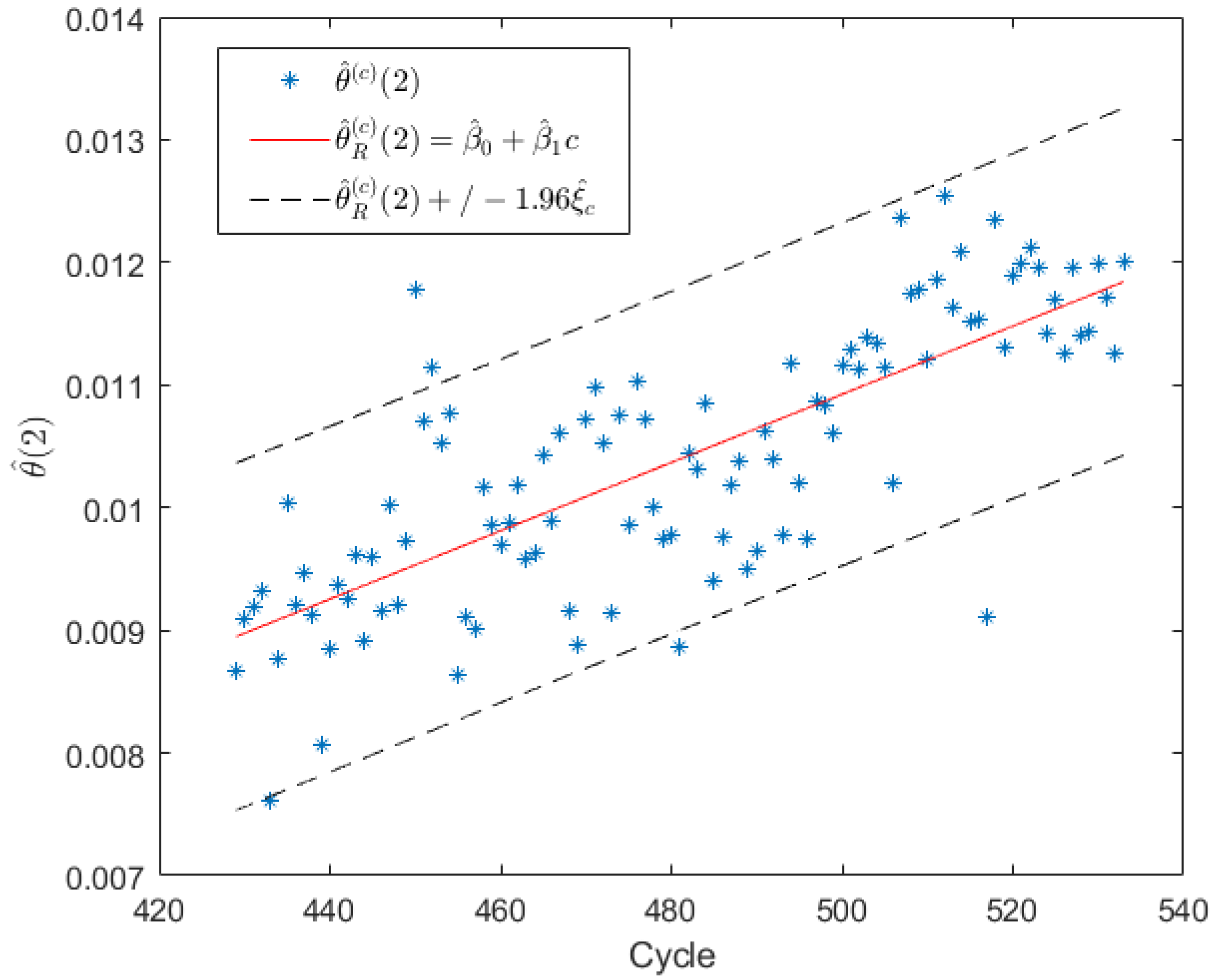
This section evaluates a potential use of the system model described in Equation (31). The elements of ${\theta }_3$ in Equation (31) were estimated for different production cycles (see Equation (22)). The elements of the estimated parameter vectors are denoted as ${\widehat{\theta }}^{\left(c\right)}\left(i\right)$, where $c=\left\{1,,2,\cdots ,n_c\right\}$ and $n_c$ is the total number of cycles.

A linear trend in ${\widehat{\theta }}^{\left(c\right)}\left(2\right)$ for the cycles $c\in [429,533]$ is observed (see Figure 5). We fitted the linear regression model

$${\widehat{\theta }}_R^{\left(c\right)}\left(2\right)={\widehat{\beta }}_0+{\widehat{\beta }}_{1}c,$$

(34)

where ${\widehat{\beta }}_0$ and ${\widehat{\beta }}_1$ are the least square estimators, and ${\widehat{\theta }}_R^{\left(c\right)}\left(2\right)$ is the estimated ${\widehat{\theta }}^{\left(c\right)}\left(2\right)$ at cycle c. The confidence intervals of ${\widehat{\theta }}_R^{\left(c\right)}\left(2\right)$ were calculated using Equation (13.17) in [39], and this was achieved by assuming the residuals of Equation (34) were white Gaussian noise. In addition, we considered a confidence level of 95% by estimating ${\widehat{\xi }}_c$ using Equation (13.16) in [39]. The estimated relative error of 6.5% in $\widehat{\theta }\left(2\right)$ was similar to but slightly smaller than the 95% intervals shown in Figure 5. Thus, the scattering around the trend line was explained by the different error sources summarized in Table 5. The trend line reveals the aging of the valve; see ${\widehat{\theta }}_R^{\left(c\right)}\left(2\right)$ in Figure 5.

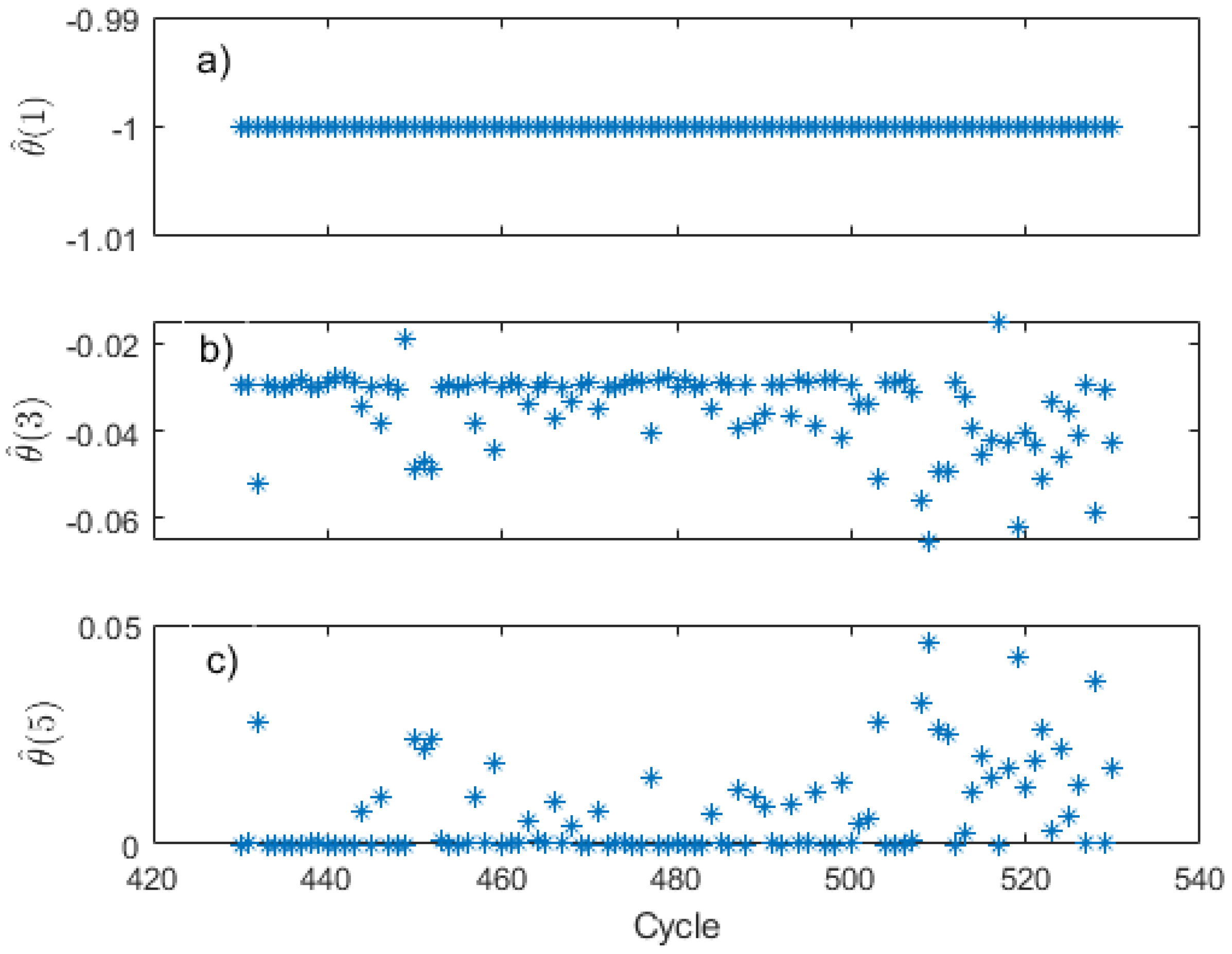
Figure 6 shows the values of the other elements of ${\widehat{\theta }}^{\left(c\right)}$ for $c\in [429,533]$. We can see that ${\widehat{\theta }}^{\left(c\right)}\left(1\right)$ was constant over the cycles, and that it stays at the limits of the constraints defined in Section 4.1. The scattering in ${\widehat{\theta }}^{\left(c\right)}\left(3\right)$ and ${\widehat{\theta }}_3^{\left(c\right)}\left(5\right)$ shows an increasing trend with the number of cycles. The estimated parameter values of ${\widehat{\theta }}^{\left(c\right)}\left(3\right)$ are bigger in magnitude than ${\widehat{\theta }}^{\left(c\right)}\left(5\right)$ for $c\in [430,500]$. The total estimated errors of $\widehat{\theta }\left(3\right)$ and $\widehat{\theta }\left(5\right)$, as given in Table 5, describe most of the scattering of the estimated parameters ${\widehat{\theta }}^{\left(c\right)}\left(3\right)$ and ${\widehat{\theta }}^{\left(c\right)}\left(5\right)$, respectively.

5. Conclusions

An input–output model of a novel two-stage two/two proportional cartridge valve was derived from a physical model that was based on fluid mechanics, dynamics, and electrical principles. This was possible because of the relative simplicity of the device when compared with more complex systems, such as machines with multiple components [9]. Therefore, each of the model parameters could be related to the design parameters of the valve. The main difference from other two-stage cartridge valves was that the valve under study was marginally stable (cf. [23]). To our knowledge, this was the first time that a model was derived for a water two-stage proportional cartridge valve with a marginally stable main valve. Moreover, parameter estimation was performed with data that were collected in industrial conditions, with the valve operating as a subsystem of a press mill, and with the valve as the plant as a closed-loop system. Parameter estimation of a proportional cartridge valve model with data collected when the valve was operating as part of a machine in a manufacturing plant and as part of a closed-loop system has not been done before.

In this work, we did not use a sensor for $P_c\left(t\right)$, which is usually the case in other studies of similar valves [12,21,23]. This limitation was addressed successfully in the derivation of the input–output model, which was achieved by using Taylor polynomials. The closed-loop operation resulted in poor system excitation, which delivered numerical problems when applying the least squares method. This problem was solved by estimating the parameters by a convex optimization problem. The constraints of the convex optimization problem were defined based on the physics of the valve and system knowledge regarding the poles of the device. An in-depth study of the contributions to the errors of the estimated parameters from different error sources were carried out.

The identified model of the valve showed that the non-linear terms were not negligible compared with the linear ones. Thus, a non-linear controller of the valve position could improve the performance of the closed-loop system compared with a linear controller. The estimated parameters of the model showed several trends vs. the production cycles. In particular, the parameter $\theta \left(2\right)$ of the input–output model in Equation (32) shows a linear trend in Figure 5 vs. the production cycles. The trend was significant compared with the estimated model errors and the scattering in the data. Analyses of more data should be carried out to check whether a prognosis of the valve’s health status could be identified. In future studies, the developed method could be used to investigate and identify different failure models of the valve, such as for leakages.

References

- Tao, F.; Zhang, H.; Liu, A.; Nee, A.Y. Digital twin in industry: State-of-the-art. IEEE Trans. Ind. Inform. 2018, 15, 2405–2415. [Google Scholar] [CrossRef]
- Wright, L.; Davidson, S. How to tell the difference between a model and a digital twin. Adv. Model. Simul. Eng. Sci. 2020, 7, 1–13. [Google Scholar] [CrossRef]
- Roy, R.B.; Mishra, D.; Pal, S.K.; Chakravarty, T.; Panda, S.; Chandra, M.G.; Pal, A.; Misra, P.; Chakravarty, D.; Misra, S. Digital twin: Current scenario and a case study on a manufacturing process. Int. J. Adv. Manuf. Technol. 2020, 107, 3691–3714. [Google Scholar] [CrossRef]
- He, B.; Bai, K.J. Digital twin-based sustainable intelligent manufacturing: A review. Adv. Manuf. 2021, 9, 1–21. [Google Scholar] [CrossRef]
- Rituraj, R.; Scheidl, R. Towards digital twin development of counterbalance valves: Modelling and experimental investigation. Mech. Syst. Signal Process. 2023, 188, 110049. [Google Scholar] [CrossRef]
- Xiang, F.; Zhi, Z.; Jiang, G. Digital twins technolgy and its data fusion in iron and steel product life cycle. In Proceedings of the 2018 IEEE 15th International Conference on Networking, Sensing and Control (ICNSC), Zhuhai, China, 27–29 March 2018; pp. 1–5. [Google Scholar]
- Karandaev, A.S.; Gasiyarov, V.R.; Radionov, A.A.; Loginov, B.M. Development of digital models of interconnected electrical profiles for rolling–drawing wire mills. Machines 2021, 9, 54. [Google Scholar] [CrossRef]
- Gasiyarova, O.A.; Karandaev, A.S.; Erdakov, I.N.; Loginov, B.M.; Khramshin, V.R. Developing digital observer of angular gaps in rolling stand mechatronic system. Machines 2022, 10, 141. [Google Scholar] [CrossRef]
- Gonzalez, O.B.; Rönnow, D. Time series modelling of a radial-axial ring rolling system. Int. J. Model. Identif. Control 2023, 43, 13–25. [Google Scholar] [CrossRef]
- Gonzalez, O.B.; Rönnow, D. A Study of OBF-ARMAX Performance for Modelling of a Mechanical System Excited by a Low Frequency Signal for Condition Monitoring. In Proceedings of the European Workshop on Advanced Control and Diagnosis, Nancy, France, 16–18 November 2022; Springer: Cham, Switzerland, 2022; pp. 73–82. [Google Scholar]
- Manring, N.D.; Fales, R.C. Hydraulic Control Systems; John Wiley & Sons: Hoboken, NJ, USA, 2019. [Google Scholar]
- Han, M.; Liu, Y.; Wu, D.; Tan, H.; Li, C. Numerical analysis and optimisation of the flow forces in a water hydraulic proportional cartridge valve for injection system. IEEE Access 2018, 6, 10392–10401. [Google Scholar] [CrossRef]
- Liu, Z.; Li, L.; Yue, D.; Wei, L.; Liu, C.; Zuo, X. Dynamic Performance Improvement of Solenoid Screw-In Cartridge Valve Using a New Hybrid Voltage Control. Machines 2022, 10, 106. [Google Scholar] [CrossRef]
- Xu, B.; Shen, J.; Liu, S.; Su, Q.; Zhang, J. Research and development of electro-hydraulic control valves oriented to industry 4.0: A review. Chin. J. Mech. Eng. 2020, 33, 1–20. [Google Scholar] [CrossRef]
- Tamburrano, P.; Plummer, A.R.; Distaso, E.; Amirante, R. A review of electro-hydraulic servovalve research and development. Int. J. Fluid Power 2018, 20, 53–98. [Google Scholar] [CrossRef]
- Liu, S.; Yao, B. Energy-saving control of single-rod hydraulic cylinders with programmable valves and improved working mode selection. SAE Trans. 2002, 111, 51–61. [Google Scholar]
- Liu, S.; Yao, B. Adaptive robust control of programmable valves with manufacturer supplied flow mapping only. In Proceedings of the 2004 43rd IEEE Conference on Decision and Control (CDC)(IEEE Cat. No. 04CH37601), Nassau, Bahamas, 14–17 December 2004; Volumne 1, pp. 1117–1122. [Google Scholar]
- Liu, S.; Yao, B. On-board system identification of systems with unknown input nonlinearity and system parameters. In Proceedings of the ASME International Mechanical Engineering Congress and Exposition, Orlando, FL, USA, 5–11 November 2005; Volume 42169, pp. 1079–1085. [Google Scholar]
- Liu, S.; Yao, B. Automated onboard modeling of cartridge valve flow mapping. IEEE/ASME Trans. Mechatron. 2006, 11, 381–388. [Google Scholar]
- Lu, L.; Yao, B.; Liu, Z. Energy saving control of a hydraulic manipulator using five cartridge valves and one accumulator. IFAC Proc. Vol. 2013, 46, 84–90. [Google Scholar] [CrossRef]
- Xu, B.; Ding, R.; Zhang, J.; Su, Q. Modeling and dynamic characteristics analysis on a three-stage fast-response and large-flow directional valve. Energy Convers. Manag. 2014, 79, 187–199. [Google Scholar] [CrossRef]
- Yue, D.; Li, L.; Wei, L.; Liu, Z.; Liu, C.; Zuo, X. Effects of pulse voltage duration on open–close dynamic characteristics of solenoid screw-In cartridge valves. Processes 2021, 9, 1722. [Google Scholar] [CrossRef]
- Han, M.; Liu, Y.; Zheng, K.; Ding, Y.; Wu, D. Investigation on the modeling and dynamic characteristics of a fast-response and large-flow water hydraulic proportional cartridge valve. Proc. Inst. Mech. Eng. Part C J. Mech. Eng. Sci. 2020, 234, 4415–4432. [Google Scholar] [CrossRef]
- Ljung, L. System identification. In Signal Analysis and Prediction; Springer: Berlin/Heidelberg, Germany, 1998; pp. 163–173. [Google Scholar]
- Zhang, J.; Lu, Z.; Xu, B.; Su, Q. Investigation on the dynamic characteristics and control accuracy of a novel proportional directional valve with independently controlled pilot stage. ISA Trans. 2019, 93, 218–230. [Google Scholar] [CrossRef]
- Li, C.; Lyu, L.; Helian, B.; Chen, Z.; Yao, B. Precision motion control of an independent metering hydraulic system with nonlinear flow modeling and compensation. IEEE Trans. Ind. Electron. 2021, 69, 7088–7098. [Google Scholar] [CrossRef]
- Lu, Z.; Zhang, J.; Xu, B.; Wang, D.; Su, Q.; Qian, J.; Yang, G.; Pan, M. Deadzone compensation control based on detection of micro flow rate in pilot stage of proportional directional valve. ISA Trans. 2019, 94, 234–245. [Google Scholar] [CrossRef] [PubMed]
- Li, Y.; Wang, Q. Adaptive robust tracking control of a proportional pressure-reducing valve with dead zone and hysteresis. Trans. Inst. Meas. Control 2018, 40, 2151–2166. [Google Scholar] [CrossRef]
- Folgheraiter, M. A combined B-spline-neural-network and ARX model for online identification of nonlinear dynamic actuation systems. Neurocomputing 2016, 175, 433–442. [Google Scholar] [CrossRef]
- Tørdal, S.S.; Klausen, A.; Bak, M.K. Experimental system identification and black box modeling of hydraulic directional control valve. Model. Identif. Control 2015, 36, 225–235. [Google Scholar] [CrossRef]
- Kilic, E.; Dolen, M.; Koku, A.B.; Caliskan, H.; Balkan, T. Accurate pressure prediction of a servo-valve controlled hydraulic system. Mechatronics 2012, 22, 997–1014. [Google Scholar] [CrossRef]
- Alimonti, C. Experimental characterization of globe and gate valves in vertical gas–liquid flows. Exp. Therm. Fluid Sci. 2014, 54, 259–266. [Google Scholar] [CrossRef]
- Munson, B.R.; Okiishi, T.H.; Huebsch, W.W.; Rothmayer, A.P. Fluid Mechanics; Wiley: Singapore, 2013. [Google Scholar]
- Atkinson, K. An Introduction to Numerical Analysis; John Wiley & Sons: Hoboken, NJ, USA, 1991. [Google Scholar]
- Boyd, S.P.; Vandenberghe, L. Convex Optimization; Cambridge University Press: Cambridge, MA, USA, 2004. [Google Scholar]
- Grant, M.; Boyd, S.; Ye, Y. CVX: Matlab Software for Disciplined Convex Programming, version 2.0 Beta. 2009. Available online: https://cvxr.com/cvx (accessed on 10 March 2024).
- Grant, M.C.; Boyd, S.P. Graph implementations for nonsmooth convex programs. In Recent Advances in Learning and Control; Springer: London, UK, 2008; pp. 95–110. [Google Scholar]
- Stoica, P.; Söderström, T. System Identification; Prentice-Hall International: Upper Saddle River, NJ, USA, 1989. [Google Scholar]
- Wasserman, L. All of Statistics: A Concise Course in Statistical Inference; Springer: Berlin/Heidelberg, Germany, 2004; Volume 26. [Google Scholar]
Figure 1.
Mechanical scheme of the device. (I) Proportional pilot valves for the flow-in to the main valve; (II) proportional pilot valves for the flow-out to the main valve; (III) emergency valve; (IV) main valve’s spindle; (V) LDTV sensor of the main valve; (VI) entrance of the hydraulic circuit to the pilot stage; (VII) hydraulic exit of the pilot stage; (VIII) and (IX) are the entrance and exit of the main valve, respectively; and (X) and (XI) are the lower and upper chambers of the main valve, respectively. The hydraulic circuit of the main valve is marked in red, the pressurized fluid of the hydraulic circuit through the pilot valves is marked in yellow, and the fluid from the pilot stage to the reservoir is marked in blue. The spindle is at its highest position. The image in the left-bottom corner shows the pilot valves and the emergency valves in the steel manufacturing plant.
Figure 2.
Diagram of the device. (I) Proportional pilot valves for the flow-in to the main valve; (II) proportional pilot valves for the flow-out to the main valve; (IV) main valve’s spindle; (VI) entrance hydraulic circuit to the pilot valves; (VII) exit hydraulic circuit of the pilot valves; and (X) and (XI) are the lower and upper chamber of the main valve, respectively. The two spindle’s cross-sectional areas are found to be different, i.e., where is smaller than . The blue solid line in the lower chamber defines the control volume in the main valve, which deforms according to x. The yellow and gray colors indicate the fluid (water) and the solid piston (steel), respectively.
Figure 3.
Signals vs. time during operation. (a) Position signal x for the spindle of the main valve (IV). (b) Voltage V applied to the solenoid of the pilot valves (I) and (II), i.e., and , respectively. (c) Pressure at (VI) and (XI). (d) Pressure at (VIII) and (IX). The changes in operating conditions ((i), (ii), and (iii)) are indicated in the figure by vertical lines.
Figure 4.
Modeling results with the validation data: (a) the measured output (position of (IV)) and the modeled output described in Equation (31) and computed with defined in Equation (32) with parameter values shown in Table 1; (b) the normalized input signals and ; (c) the error signal obtained by subtracting from .
Figure 5.
The parameter vs. cycle. Note the red fitted line plotting Equation (34) and the 95% confidence interval.
Figure 6.
The elements of vs. cycle. (a) vs. cycle, (b) vs. cycle, and (c) vs. cycle.