

Comprehensive Study of Compression and Texture Integration for Digital Imaging and Communications in Medicine Data Analysis
Abstract
:
1. Introduction
2. Materials and Methods
2.1. Mathematical Framework for Extraction of the ROI and NROI
2.2. Features Derived from the
2.3. Classification of the Image Compression Algorithm
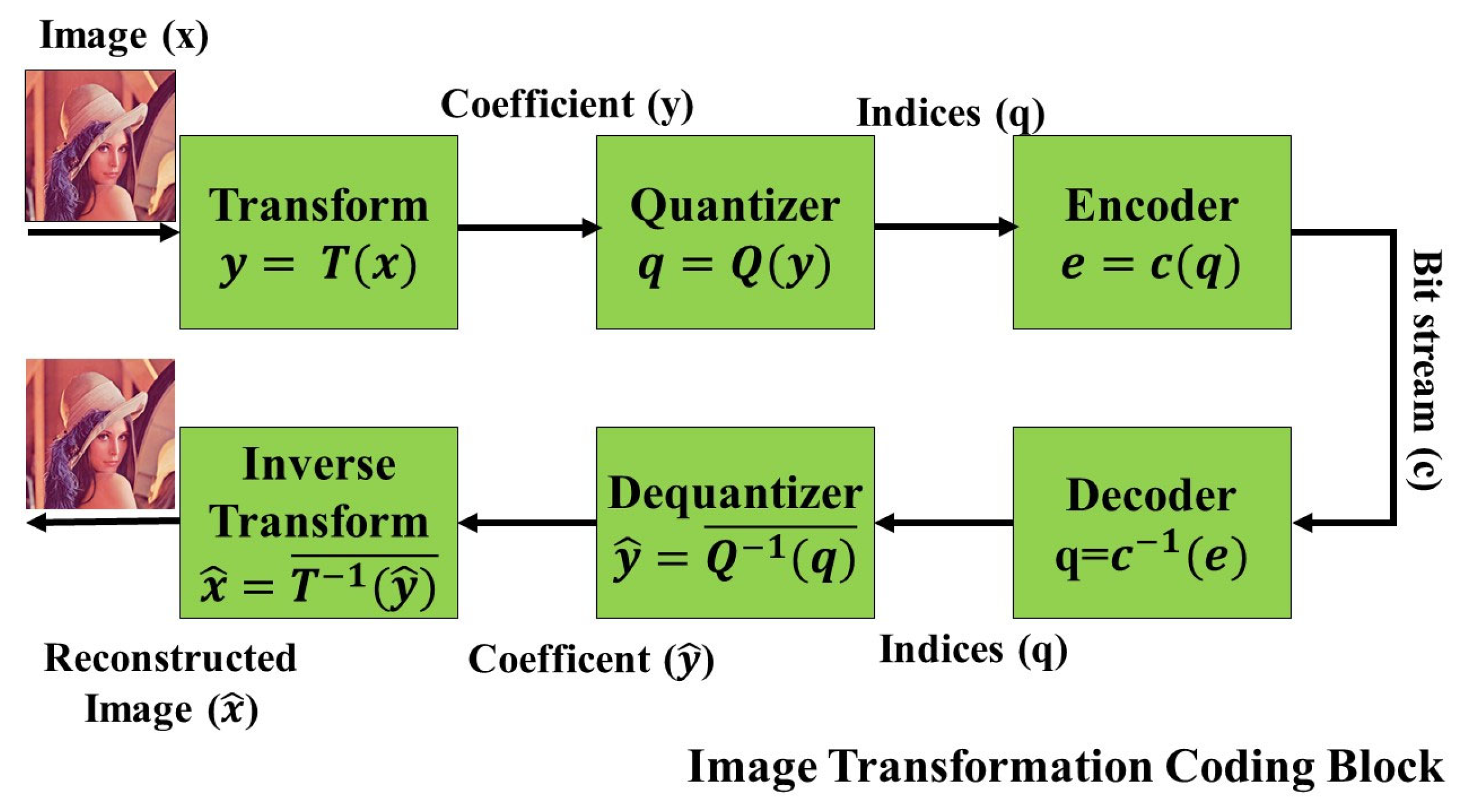
2.3.1. Transform Coding
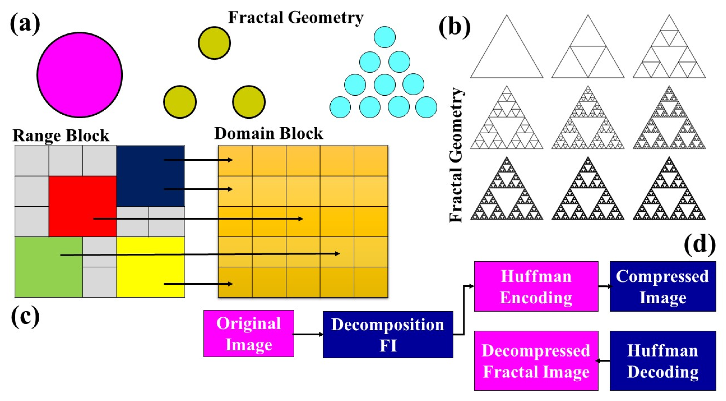
2.3.2. Fractal Compression
- The achievable compression ratios range from 1:4 to 1:100, making it efficient in reducing data size.
- The compression phase is notably slower compared with other methodologies.
- Decoding, on the other hand, is expedited and is not bound by resolution constraints.
- Natural images, with their inherent similarities and patterns, are best suited for this compression method.
- The algorithm exhibits superior performance with color images as opposed to grayscale ones.
2.3.3. Chroma Sampling
2.3.4. Discrete Cosines Transform
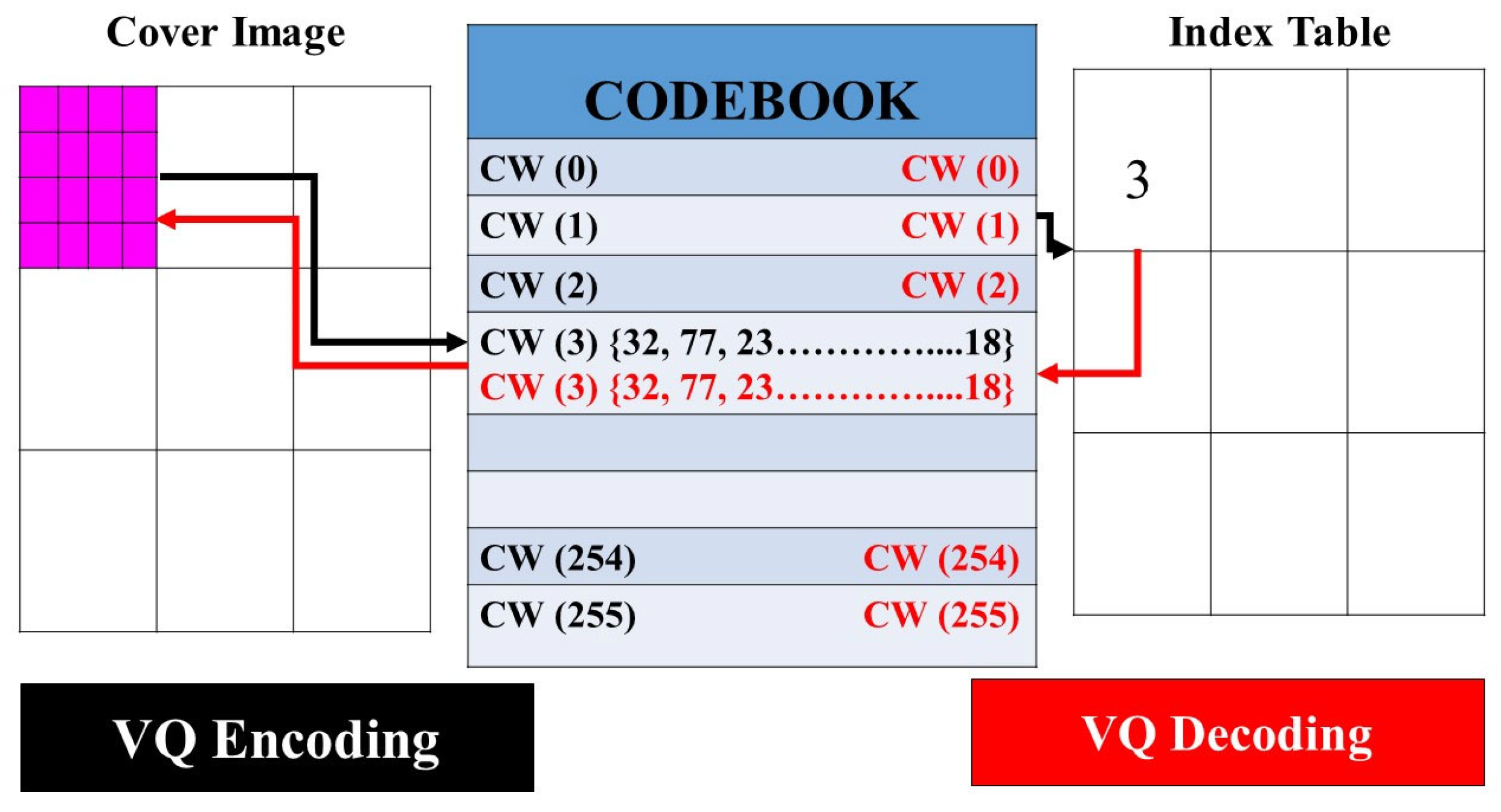
2.3.5. Vector Quantization Algorithm

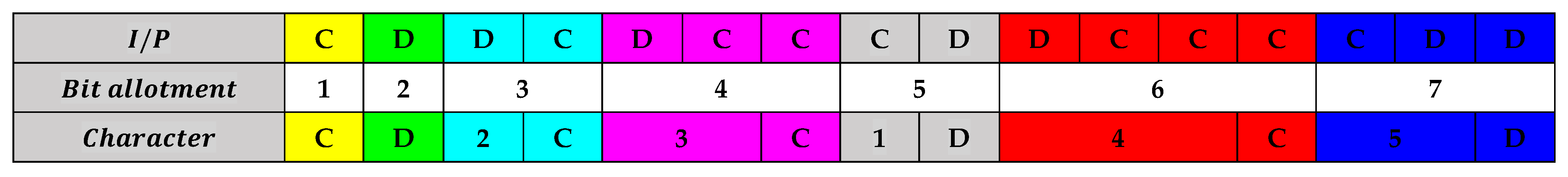
2.3.6. Run-Length Encoding
2.3.7. Entropy Encoding
2.3.8. Lempel–Ziv–Welch Image Compression
2.3.9. DEFLATE Image Compression
2.4. Performance Measures for Image Compression
2.4.1. Mean Square Error
2.4.2. The Peak Signal to Noise Ratio
2.4.3. Compression Ratio
2.4.4. Bits per Pixels
3. Results
3.1. ROI and NROI-Based Compression of the DICOM Image
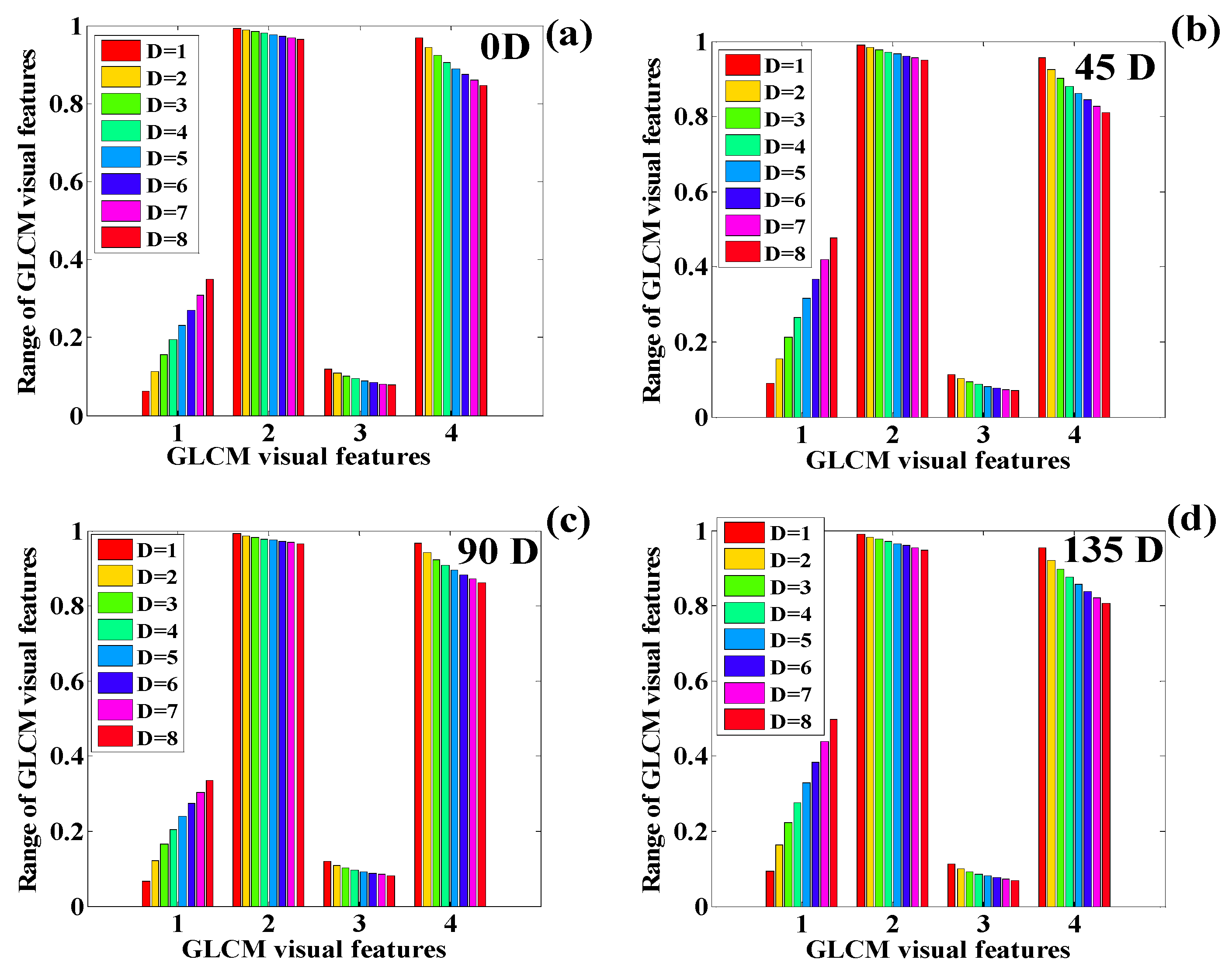
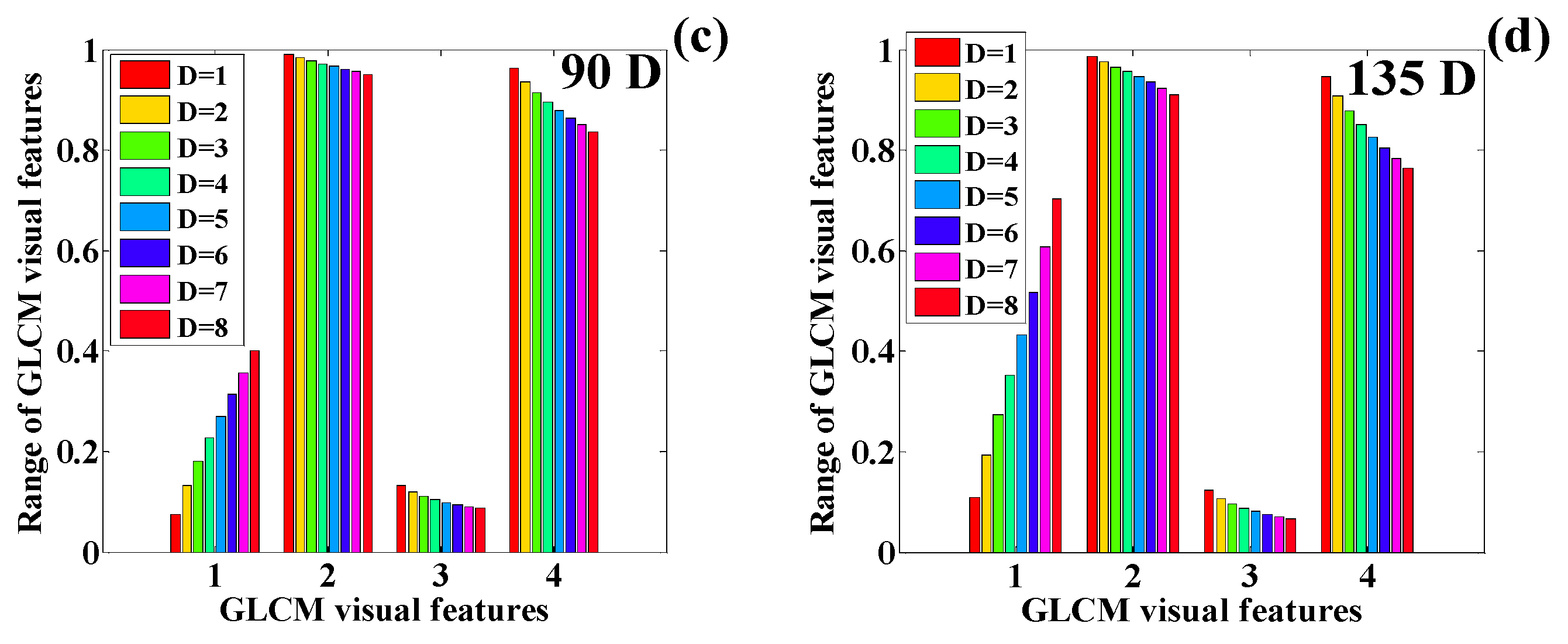
3.2. Texture Quantification of the Time-Series CT Chest Images
4. Discussion
5. Conclusions
Author Contributions
Funding
Data Availability Statement
Acknowledgments
Conflicts of Interest
References
- Grasso, M.; Klicperová-Baker, M.; Koos, S.; Kosyakova, Y.; Petrillo, A. The impact of the coronavirus crisis on European societies. What have we learned and where do we go from here?—Introduction to the COVID volume. Eur. Soc. 2021, 23, S2–S32. [Google Scholar] [CrossRef]
- Chen, S.; Prettner, K.; Kuhn, M.; Geldsetzer, P.; Wang, C.; Bärnighausen, T.; Bloom, D.E. Climate and the spread of COVID-19. Sci. Rep. 2021, 11, 9042. [Google Scholar] [CrossRef] [PubMed]
- Varotsos, C.A.; Krapivin, V.F. A new model for the spread of COVID-19 and the improvement of safety. Saf. Sci. 2020, 132, 104962. [Google Scholar] [CrossRef]
- Xu, H.; Yan, C.; Fu, Q.; Xiao, K.; Yu, Y.; Han, D.; Wang, W.; Cheng, J. Possible environmental effects on the spread of COVID-19 in China. Sci. Total Environ. 2020, 731, 139211. [Google Scholar] [CrossRef]
- Matta, S.; Chopra, K.; Arora, V. Morbidity and mortality trends of COVID-19 in top 10 countries. Indian J. Tuberc. 2020, 67, S167–S172. [Google Scholar] [CrossRef]
- Sharma, N.; Basu, S.; Sharma, P. Sociodemographic determinants of the adoption of a contact tracing application during the COVID-19 epidemic in Delhi, India. Health Policy Technol. 2021, 10, 100496. [Google Scholar] [CrossRef]
- Chakraborty, C.; Sharma, A.R.; Bhattacharya, M.; Mallik, B.; Nandi, S.S.; Lee, S.-S. Comparative genomics, evolutionary epidemiology, and RBD-hACE2 receptor binding pattern in B.1.1.7 (Alpha) and B.1.617.2 (Delta) related to their pandemic response in UK and India. Infect. Genet. Evol. 2022, 101, 105282. [Google Scholar] [CrossRef]
- Diao, B.; Wang, C.; Wang, R.; Feng, Z.; Zhang, J.; Yang, H.; Tan, Y.; Wang, H.; Wang, C.; Liu, L.; et al. Human kidney is a target for novel severe acute respiratory syndrome coronavirus 2 infection. Nat. Commun. 2021, 12, 2506. [Google Scholar] [CrossRef]
- Gordon-Dseagu, V.L.; Shelton, N.; Mindell, J. Diabetes mellitus and mortality from all-causes, cancer, cardiovascular and respiratory disease: Evidence from the Health Survey for England and Scottish Health Survey cohorts. J. Diabetes Its Complicat. 2014, 28, 791–797. [Google Scholar] [CrossRef]
- Kudlay, D.; Svistunov, A.; Satyshev, O. COVID-19 Vaccines: An Updated Overview of Different Platforms. Bioengineering 2022, 9, 714. [Google Scholar] [CrossRef]
- Sessa, M.; Kragholm, A.H.K.; Andersen, M. Thromboembolic events in younger women exposed to Pfizer-BioNTech or Moderna COVID-19 vaccines. Expert Opin. Drug Saf. 2021, 20, 1451–1453. [Google Scholar] [CrossRef]
- Singh, A.; Khillan, R.; Mishra, Y.; Khurana, S. The safety profile of COVID-19 vaccinations in the United States. Am. J. Infect. Control 2021, 50, 15–19. [Google Scholar] [CrossRef]
- Jones, I.; Roy, P. Sputnik V COVID-19 vaccine candidate appears safe and effective. Lancet 2021, 397, 671. [Google Scholar] [CrossRef]
- Pramod, S.; Govindan, D.; Ramasubramani, P.; Kar, S.S.; Aggarwal, R. Effectiveness of Covishield vaccine in preventing COVID-19—A test-negative case-control study. Vaccine 2022, 40, 3294–3297. [Google Scholar] [CrossRef]
- Parida, S.P.; Sahu, D.P.; Singh, A.K.; Alekhya, G.; Subba, S.H.; Mishra, A.; Padhy, B.M.; Patro, B.K. Adverse events following immunization of COVID-19 (Covaxin) vaccine at a tertiary care center of India. J. Med. Virol. 2022, 94, 2453–2459. [Google Scholar] [CrossRef]
- Kudlay, D.; Svistunov, A. COVID-19 Vaccines: An Overview of Different Platforms. Bioengineering 2022, 9, 72. [Google Scholar]
- Dijkstra, S.; Baas, S.; Braaksma, A.; Boucherie, R.J. Dynamic fair balancing of COVID-19 patients over hospitals based on forecasts of bed occupancy. Omega 2022, 116, 102801. [Google Scholar] [CrossRef]
- Devereaux, A.V.; Backer, H.; Salami, A.; Wright, C.; Christensen, K.; Rice, K.; Jakel-Smith, C.; Metzner, M.; Bains, J.K.; Staats, K.; et al. Oxygen and Ventilator Logistics During California’s COVID-19 Surge: When Oxygen Becomes a Scarce Resource. Disaster Med. Public Health Prep. 2021, 17, e33. [Google Scholar] [CrossRef] [PubMed]
- Fesharaki-Zadeh, A.; Lowe, N.; Arnsten, A.F. Clinical experience with the α2A-adrenoceptor agonist, guanfacine, and N-acetylcysteine for the treatment of cognitive deficits in “Long-COVID19”. Neuroimmunol. Rep. 2023, 3, 100154. [Google Scholar] [CrossRef]
- Moeti, M.; Makubalo, L.; Gueye, A.S.; Balde, T.; Karamagi, H.; Awandare, G.; Thumbi, S.M.; Zhang, F.; Mutapi, F.; Woolhouse, M. Conflicting COVID-19 excess mortality estimates. Lancet 2023, 401, 431. [Google Scholar] [CrossRef] [PubMed]
- Attallah, O. RADIC:A tool for diagnosing COVID-19 from chest CT and X-ray scans using deep learning and quad-radiomics. Chemom. Intell. Lab. Syst. 2023, 233, 104750. [Google Scholar] [CrossRef]
- Duan, L.-Y.; Liu, J.; Yang, W.; Huang, T.; Gao, W. Video Coding for Machines: A Paradigm of Collaborative Compression and Intelligent Analytics. IEEE Trans. Image Process. 2020, 29, 8680–8695. [Google Scholar] [CrossRef]
- Ni, J.Z.F.; Noori, M.N. Deep learning for data anomaly detection and data compression of a long-span suspension bridge. Comput. Aided Civ. Infrastruct. Eng. 2020, 35, 685–700. [Google Scholar] [CrossRef]
- Liu, X.; Tong, X.; Zhang, M.; Wang, Z.; Fan, Y. Image compression and encryption algorithm based on uniform non-degeneracy chaotic system and fractal coding. Nonlinear Dyn. 2023, 111, 8771–8798. [Google Scholar] [CrossRef]
- Lu, Y.; Gong, M.; Cao, L.; Gan, Z.; Chai, X.; Li, A. Exploiting 3D fractal cube and chaos for effective multi-image compression and encryption. J. King Saud Univ. Comput. Inf. Sci. 2023, 35, 37–58. [Google Scholar] [CrossRef]
- Zou, C.; Wan, S.; Ji, T.; Blanch, M.G.; Mrak, M.; Herranz, L. Chroma Intra Prediction with Lightweight Attention-Based Neural Networks. IEEE Trans. Circuits Syst. Video Technol. 2023, 34, 549–560. [Google Scholar] [CrossRef]
- Li, X.; Du, W.; Chen, D. Object extraction from image with big size based on bilateral grid. Comput. Electr. Eng. 2023, 105, 108454. [Google Scholar] [CrossRef]
- Hong, Q.; He, B.; Zhang, Z.; Xiao, P.; Du, S.; Zhang, J. Circuit Design and Application of Discrete Cosine Transform Based on Memristor. IEEE J. Emerg. Sel. Top. Circuits Syst. 2023, 13, 502–513. [Google Scholar] [CrossRef]
- Yang, Z.-C. Data-driven discrete cosine transform (DCT)-based modeling and simulation for hourly air humidity prediction. Soft Comput. 2023, 28, 541–563. [Google Scholar] [CrossRef]
- Akhtarkavan, E.; Majidi, B.; Mandegari, A. Secure Medical Image Communication Using Fragile Data Hiding Based on Discrete Wavelet Transform and A5 Lattice Vector Quantization. IEEE Access 2023, 11, 9701–9715. [Google Scholar] [CrossRef]
- Oh, Y.; Jeon, Y.-S.; Chen, M.; Saad, W. FedVQCS: Federated Learning via Vector Quantized Compressed Sensing. IEEE Trans. Wirel. Commun. 2023. Early Access. [Google Scholar] [CrossRef]
- Kim, C.; Dao, N.-N.; Jung, K.-H.; Leng, L. Dual Reversible Data Hiding in Encrypted Halftone Images Using Matrix Encoding. Electronics 2023, 12, 3134. [Google Scholar] [CrossRef]
- Cao, W.; Leng, X.; Yu, T.; Gu, X.; Liu, Q. A Joint Encryption and Compression Algorithm for Multiband Remote Sensing Image Transmission. Sensors 2023, 23, 7600. [Google Scholar] [CrossRef]
- Viknesh, C.K.; Kumar, P.N.; Seetharaman, R.; Anitha, D. Detection and Classification of Melanoma Skin Cancer Using Image Processing Technique. Diagnostics 2023, 13, 3313. [Google Scholar] [CrossRef]
- Cui, M.; Li, K.; Li, Y.; Kamuhanda, D.; Tessone, C.J. Semi-Supervised Semantic Segmentation of Remote Sensing Images Based on Dual Cross-Entropy Consistency. Entropy 2023, 25, 681. [Google Scholar] [CrossRef] [PubMed]
- Bhatia, S.; Almutairi, A. A Robust Fuzzy Equilibrium Optimization-Based ROI Selection and DWT-Based Multi-Watermarking Model for Medical Images. Sustainability 2023, 15, 6189. [Google Scholar] [CrossRef]
- Livada, Č.; Horvat, T.; Baumgartner, A. Novel Block Sorting and Symbol Prediction Algorithm for PDE-Based Lossless Image Compression: A Comparative Study with JPEG and JPEG 2000. Appl. Sci. 2023, 13, 3152. [Google Scholar] [CrossRef]
- Sui, L.; Li, H.; Liu, J.; Xiao, Z.; Tian, A. Reversible Data Hiding in Encrypted Images Based on Hybrid Prediction and Huffman Coding. Symmetry 2023, 15, 1222. [Google Scholar] [CrossRef]
- Daoui, A.; Mao, H.; Yamni, M.; Li, Q.; Alfarraj, O.; El-Latif, A.A.A. Novel Integer Shmaliy Transform and New Multiparametric Piecewise Linear Chaotic Map for Joint Lossless Compression and Encryption of Medical Images in IoMTs. Mathematics 2023, 11, 3619. [Google Scholar] [CrossRef]
- Parikh, S.S.; Ruiz, D.; Kalva, H.; Fernández-Escribano, G.; Adzic, V. High Bit-Depth Medical Image Compression with HEVC. IEEE J. Biomed. Health Inform. 2018, 22, 552–560. [Google Scholar] [CrossRef]
- Rahmat, R.F.; Andreas, T.S.M.; Fahmi, F.; Pasha, M.F.; Alzahrani, M.Y.; Budiarto, R. Analysis of DICOM Image Compression Alternative Using Huffman Coding. J. Healthc. Eng. 2019, 2019, 5810540. [Google Scholar] [CrossRef]
- Ammah, P.N.T.; Owusu, E. Robust medical image compression based on wavelet transform and vector quantization. Inform. Med. Unlocked 2019, 15, 100183. [Google Scholar] [CrossRef]
- Sunil, H.; Hiremath, S.G. A combined scheme of pixel and block level splitting for medical image compression and reconstruction. Alex. Eng. J. 2018, 57, 767–772. [Google Scholar] [CrossRef]
- Voigt, M.; Miller, J.A.; Mainza, A.N.; Bam, L.C.; Becker, M. The Robustness of the Gray Level Co-Occurrence Matrices and X-Ray Computed Tomography Method for the Quantification of 3D Mineral Texture. Minerals 2020, 10, 334. [Google Scholar] [CrossRef]
- Yan, Z.; Ma, L.; He, W.; Zhou, L.; Lu, H.; Liu, G.; Huang, G. Comparing Object-Based and Pixel-Based Methods for Local Climate Zones Mapping with Multi-Source Data. Remote Sens. 2022, 14, 3744. [Google Scholar] [CrossRef]
- Humeau-Heurtie, A. Texture Feature Extraction Methods: A Survey. IEEE Access 2019, 7, 8975–9000. [Google Scholar] [CrossRef]
- Alpaslan, N.; Hanbay, K. Multi-Resolution Intrinsic Texture Geometry-Based Local Binary Pattern for Texture Classification. IEEE Access 2020, 8, 54415–54430. [Google Scholar] [CrossRef]
- Ramola, A.; Shakya, A.K.; Van Pham, D. Study of statistical methods for texture analysis and their modern evolutions. Eng. Rep. 2020, 2, e12149. [Google Scholar] [CrossRef]
- Kaplan, K.; Kaya, Y.; Kuncan, M.; Ertunç, H.M. Brain tumor classification using modified local binary patterns (LBP) feature extraction methods. Med. Hypotheses 2020, 139, 109696. [Google Scholar] [CrossRef]
- Chen, S.; Zhong, S.; Xue, B.; Li, X.; Zhao, L.; Chang, C.-I. Iterative Scale-Invariant Feature Transform for Remote Sensing Image Registration. IEEE Trans. Geosci. Remote. Sens. 2020, 59, 3244–3265. [Google Scholar] [CrossRef]
- Gupta, S.; Thakur, K.; Kumar, M. 2D-human face recognition using SIFT and SURF descriptors of face’s feature regions. Vis. Comput. 2020, 37, 447–456. [Google Scholar] [CrossRef]
- Nayak, S.R.; Mishra, J.; Palai, G. Analysing roughness of surface through fractal dimension: A review. Image Vis. Comput. 2019, 89, 21–34. [Google Scholar] [CrossRef]
- Gozum, M.M.; Serhat, G.; Basdogan, I. A semi-analytical model for dynamic analysis of non-uniform plates. Appl. Math. Model. 2019, 76, 883–899. [Google Scholar] [CrossRef]
- Shakya, A.K.; Ramola, A.; Pandey, D.C. Polygonal region of interest-based compression of DICOM images. In Proceedings of the International Conference on Computing Communication and Automation (ICCCA), Noida, India, 5–6 May 2017. [Google Scholar]
- Haralick, R.M.; Shanmugam, K.; Dinstein, I. Textural Features for Image Classification. IEEE Trans. Syst. Man Cybern. 1973, SMC-3, 610–621. [Google Scholar] [CrossRef]
- Gotlieb, C.C.; Kreyszig, H.E. Texture descriptors based on co-occurrence matrices. Comput. Vis. Graph. Image Process. 1990, 51, 70–86. [Google Scholar] [CrossRef]
- Zhao, J.; Wang, S.; Zhang, L. Block Image Encryption Algorithm Based on Novel Chaos and DNA Encoding. Information 2023, 14, 150. [Google Scholar] [CrossRef]
- Wang, J.; Tan, F.S.; Yuan, Y. Random Matrix Transformation and Its Application in Image Hiding. Sensors 2023, 23, 1017. [Google Scholar] [CrossRef]
- Starosolski, R. Hybrid Adaptive Lossless Image Compression Based on Discrete Wavelet Transform. Entropy 2020, 22, 751. [Google Scholar] [CrossRef]
- Petráš, I. Novel Low-Pass Two-Dimensional Mittag–Leffler Filter and Its Application in Image Processing. Fractal Fract. 2023, 7, 881. [Google Scholar] [CrossRef]
- Aldakheel, E.A.; Khafaga, D.S.; Fathi, I.S.; Hosny, K.M.; Hassan, G. Efficient Analysis of Large-Size Bio-Signals Based on Orthogonal Generalized Laguerre Moments of Fractional Orders and Schwarz–Rutishauser Algorithm. Fractal Fract. 2023, 7, 826. [Google Scholar] [CrossRef]
- Kumar, R.S.; Manimegalai, P. Near lossless image compression using parallel fractal texture identification. Biomed. Signal Process. Control. 2020, 58, 101862. [Google Scholar] [CrossRef]
- Wiseman, Y. Adapting the H.264 Standard to the Internet of Vehicles. Technologies 2023, 11, 103. [Google Scholar] [CrossRef]
- Babu, C.; Chandy, D.A.; Karthigaikumar, P. Novel chroma subsampling patterns for wireless capsule endoscopy compression. Neural Comput. Appl. 2019, 32, 6353–6362. [Google Scholar] [CrossRef]
- Heindel, A.; Prestele, B.; Gehlert, A.; Kaup, A. Enhancement Layer Coding for Chroma Sub-Sampled Screen Content Video. IEEE Trans. Circuits Syst. Video Technol. 2021, 32, 788–801. [Google Scholar] [CrossRef]
- Lin, T.-L.; Liu, B.-H.; Jiang, K.-H. An Efficient Algorithm for Luminance Optimization in Chroma Downsampling. IEEE Trans. Circuits Syst. Video Technol. 2020, 31, 3719–3724. [Google Scholar] [CrossRef]
- Baracchi, D.; Shullani, D.; Iuliani, M.; Giani, D.; Piva, A. Camera Obscura: Exploiting in-camera processing for image counter forensics. Forensic Sci. Int. Digit. Investig. 2021, 38, 301213. [Google Scholar] [CrossRef]
- Zhu, Y.; Fan, L.; Li, Q.; Chang, J. Multi-Scale Discrete Cosine Transform Network for Building Change Detection in Very-High-Resolution Remote Sensing Images. Remote Sens. 2023, 15, 5243. [Google Scholar] [CrossRef]
- Liu, H.; Zhang, X.; Dong, H.; Liu, Z.; Hu, X. Magnetic Anomaly Detection Based on Energy-Concentrated Discrete Cosine Wavelet Transform. IEEE Trans. Instrum. Meas. 2023, 72, 9700210. [Google Scholar] [CrossRef]
- Linde, Y.; Buzo, A.; Gray, R. An Algorithm for Vector Quantizer Design. IEEE Trans. Commun. 1980, 28, 84–95. [Google Scholar] [CrossRef]
- Fadel, M.M.; Said, W.; Hagras, E.A.A.; Arnous, R. A Fast and Low Distortion Image Steganography Framework Based on Nature-Inspired Optimizers. IEEE Access 2023, 11, 125768–125789. [Google Scholar] [CrossRef]
- Soni, E.; Nagpal, A.; Garg, P.; Pinheiro, P.R. Assessment of Compressed and Decompressed ECG Databases for Telecardiology Applying a Convolution Neural Network. Electronics 2022, 11, 2708. [Google Scholar] [CrossRef]
- Chianphatthanakit, C.; Boonsongsrikul, A.; Suppharangsan, S. Differential Run-Length Encryption in Sensor Networks. Sensors 2019, 19, 3190. [Google Scholar] [CrossRef]
- Dai, B.; Yin, S.; Gao, Z.; Wang, K.; Zhang, D.; Zhuang, S.; Wang, X. Data Compression for Time-Stretch Imaging Based on Differential Detection and Run-Length Encoding. J. Light. Technol. 2017, 35, 5098–5104. [Google Scholar] [CrossRef]
- Ahmed, K.; Nadeem, M.I.; Li, D.; Zheng, Z.; Ghadi, Y.Y.; Assam, M.; Mohamed, H.G. Exploiting Stacked Autoencoders for Improved Sentiment Analysis. Appl. Sci. 2022, 12, 12380. [Google Scholar] [CrossRef]
- Kumar, B.S.; Manjunath, A.; Christopher, S. Improved entropy encoding for high efficient video coding standard. Alex. Eng. J. 2018, 57, 1–9. [Google Scholar] [CrossRef]
- Rahman, M.A.; Hamada, M. Lossless Image Compression Techniques: A State-of-the-Art Survey. Symmetry 2019, 11, 1274. [Google Scholar] [CrossRef]
- Hwang, G.B.; Cho, K.N.; Han, C.Y.; Oh, H.W.; Yoon, Y.H.; Lee, S.E. Lossless Decompression Accelerator for Embedded Processor with GUI. Micromachines 2021, 12, 145. [Google Scholar] [CrossRef]
- Tu, K.; Puchala, D. Variable-to-Variable Huffman Coding: Optimal and Greedy Approaches. Entropy 2022, 24, 1447. [Google Scholar] [CrossRef]
- Shubham, S.; Bhandari, A.K. A generalized Masi entropy based efficient multilevel thresholding method for color image segmentation. Multimed. Tools Appl. 2019, 78, 17197–17238. [Google Scholar] [CrossRef]
- Zemliachenko, A.N.; Kozhemiakin, R.A.; Abramov, S.K.; Lukin, V.V.; Vozel, B.; Chehdi, K.; Egiazarian, K.O. Prediction of Compression Ratio for DCT-Based Coders with Application to Remote Sensing Images. IEEE J. Sel. Top. Appl. Earth Obs. Remote. Sens. 2017, 11, 257–270. [Google Scholar] [CrossRef]
- S.A. Center. Center for Artificial Intelligence in Medicine & Imaging. Stanford Ford University. 2023. Available online: https://aimi.stanford.edu/shared-datasets (accessed on 1 November 2023).
- M. I. &. T. A. (MITA). About DICOM: Overview. NEMA. 1 January 2001. Available online: https://www.dicomstandard.org/about-home (accessed on 27 August 2021).
- Halford, J.J.; Clunie, D.A.; Brinkmann, B.H.; Krefting, D.; Rémi, J.; Rosenow, F.; Husain, A.; Fürbass, F.; Ehrenberg, J.A.; Winkler, S. Standardization of neurophysiology signal data into the DICOM® standard. Clin. Neurophysiol. 2021, 132, 993–997. [Google Scholar] [CrossRef]
- GNU. GNU Operating System. April 2022. Available online: https://www.gnu.org/licenses/ (accessed on 30 August 2023).
- I. S. o. Radiology. Italian Society of Radiology. 10 February 2002. Available online: https://sirm.org/en/who-we-are/ (accessed on 30 August 2023).
- Dumas, T.; Roumy, A.; Guillemot, C. Context-Adaptive Neural Network-Based Prediction for Image Compression. IEEE Trans. Image Process. 2019, 29, 679–693. [Google Scholar] [CrossRef]
- Ma, S.; Zhang, X.; Jia, C.; Zhao, Z.; Wang, S.; Wang, S. Image and Video Compression With Neural Networks: A Review. IEEE Trans. Circuits Syst. Video Technol. 2020, 30, 1683–1698. [Google Scholar] [CrossRef]
- Zhou, Y.; Yen, G.G.; Yi, Z. Evolutionary Compression of Deep Neural Networks for Biomedical Image Segmentation. IEEE Trans. Neural Netw. Learn. Syst. 2020, 31, 2916–2929. [Google Scholar] [CrossRef]
- Zhou, Y.; Yen, G.G.; Yi, Z. A Knee-Guided Evolutionary Algorithm for Compressing Deep Neural Networks. IEEE Trans. Cybern. 2019, 51, 1626–1638. [Google Scholar] [CrossRef]
- Daradkeh, Y.I.; Tvoroshenko, I.; Gorokhovatskyi, V.; Latiff, L.A.; Ahmad, N. Development of Effective Methods for Structural Image Recognition Using the Principles of Data Granulation and Apparatus of Fuzzy Logic. IEEE Access 2021, 9, 13417–13428. [Google Scholar] [CrossRef]
- Liu, D.; Huang, X.; Zhan, W.; Ai, L.; Zheng, X.; Cheng, S. View synthesis-based light field image compression using a generative adversarial network. Inf. Sci. 2020, 545, 118–131. [Google Scholar] [CrossRef]
- Jiang, F.; Lu, Y.; Chen, Y.; Cai, D.; Li, G. Image recognition of four rice leaf diseases based on deep learning and support vector machine. Comput. Electron. Agric. 2020, 179, 105824. [Google Scholar] [CrossRef]
- Li, X.; Shi, J.; Chen, Z. Task-Driven Semantic Coding via Reinforcement Learning. IEEE Trans. Image Process. 2021, 30, 6307–6320. [Google Scholar] [CrossRef] [PubMed]
- Wang, P.; Fan, E.; Wang, P. Comparative analysis of image classification algorithms based on traditional machine learning and deep learning. Pattern Recognit. Lett. 2021, 141, 61–67. [Google Scholar] [CrossRef]
- Cheng, Z.; Sun, H.; Takeuchi, M.; Katto, J. Energy Compaction-Based Image Compression Using Convolutional AutoEncoder. IEEE Trans. Multimed. 2019, 22, 860–873. [Google Scholar] [CrossRef]
- Cui, M.; Zhang, D.Y. Artificial intelligence and computational pathology. Lab. Investig. 2021, 101, 412–422. [Google Scholar] [CrossRef] [PubMed]
- Barragán-Montero, A.; Javaid, U.; Valdés, G.; Nguyen, D.; Desbordes, P.; Macq, B.; Willems, S.; Vandewinckele, L.; Holmström, M.; Löfman, F.; et al. Artificial intelligence and machine learning for medical imaging: A technology review. Phys. Medica 2021, 83, 242–256. [Google Scholar] [CrossRef] [PubMed]


| Chroma Subsampling | Features | Ref. |
|---|---|---|
| In this sampling methodology, all three components have the same sampling rate as the input resolution. | [65,66] | |
| In this sampling methodology, chroma subcomponents are sampled by a factor of 2, and their influential position is co-sited. | [65,66] | |
| In this sampling methodology, and components are sampled by a factor of 4 horizontally and co-sited with the fourth brightness sample. | [65,66] | |
| In this sampling methodology, and components are subsampled by a factor of 2 in both the horizontal and vertical directions. | [65,66] | |
| This sampling methodology uses half of the vertical and one-fourth of the horizontal color resolution along with one-eighthof the bandwidth of the maximum color resolution. | [65,66] | |
| In this sampling methodology, and components are subsampled by a factor of 3 horizontally. The chroma sample is later divided by every third brightness sample. The 36-byte elements are also reduced by 20, producing compression. | [66,67] |
| S. No | Series | Scan Mode | mAs | KV | N*T | CTDIvo (mGy) | DLP (mGy*cm) | Phantom Type (cm) |
|---|---|---|---|---|---|---|---|---|
| 1 | Mediastin | Surview | ----- | 120 | 2 × 0.75 | 0.05 | 1.93 | BODY32 |
| 2 | Mediastin | Helical | 80 | 120 | 16 × 1.50 | 5.55 | 170.49 | BODY32 |
| S. No | NROI | Image Compression Algorithm | MSE | PSNR | BPP | CR | CT* (s) | DCT* (s) |
|---|---|---|---|---|---|---|---|---|
| 1 | Figure 16a | Discrete cosine transform (DCT) | 0.0018 | 123.77 | 0.574 | 27.87 | 1.33 | 22.1 |
| 2 | Figure 16b | 0.0054 | 119.00 | 0.512 | 31.25 | 1.38 | 24.9 | |
| 3 | Figure 16c | 0.0652 | 108.18 | 0.482 | 33.19 | 1.41 | 26.4 | |
| 4 | Figure 16d | 0.3847 | 100.47 | 0.464 | 34.48 | 1.49 | 28.2 | |
| 5 | Figure 16a | Discrete wavelet transform (DWT) | 0.0008 | 127.29 | 0.422 | 37.91 | 1.51 | 23.1 |
| 6 | Figure 16b | 0.0032 | 121.29 | 0.389 | 41.13 | 1.58 | 25.6 | |
| 7 | Figure 16c | 0.0315 | 111.35 | 0.302 | 52.98 | 1.62 | 27.8 | |
| 8 | Figure 16d | 0.2752 | 101.93 | 0.232 | 68.96 | 1.68 | 28.4 | |
| 9 | Figure 16a | Fractal compression algorithm (FCA) | 0.0009 | 126.78 | 0.481 | 33.26 | 1.34 | 25.9 |
| 10 | Figure 16b | 0.0084 | 117.08 | 0.432 | 37.03 | 1.38 | 26.8 | |
| 11 | Figure 16c | 0.0542 | 108.98 | 0.354 | 45.19 | 1.45 | 27.7 | |
| 12 | Figure 16d | 0.4842 | 99.47 | 0.264 | 60.60 | 1.51 | 28.9 | |
| 13 | Figure 16a | Vector quantization algorithm (VQA) | 0.0012 | 125.53 | 0.584 | 27.39 | 1.23 | 21.4 |
| 14 | Figure 16b | 0.0048 | 119.51 | 0.512 | 31.25 | 1.36 | 24.5 | |
| 15 | Figure 16c | 0.0568 | 108.78 | 0.482 | 33.19 | 1.48 | 28.5 | |
| 16 | Figure 16d | 0.3218 | 101.25 | 0.413 | 38.74 | 1.55 | 31.5 |
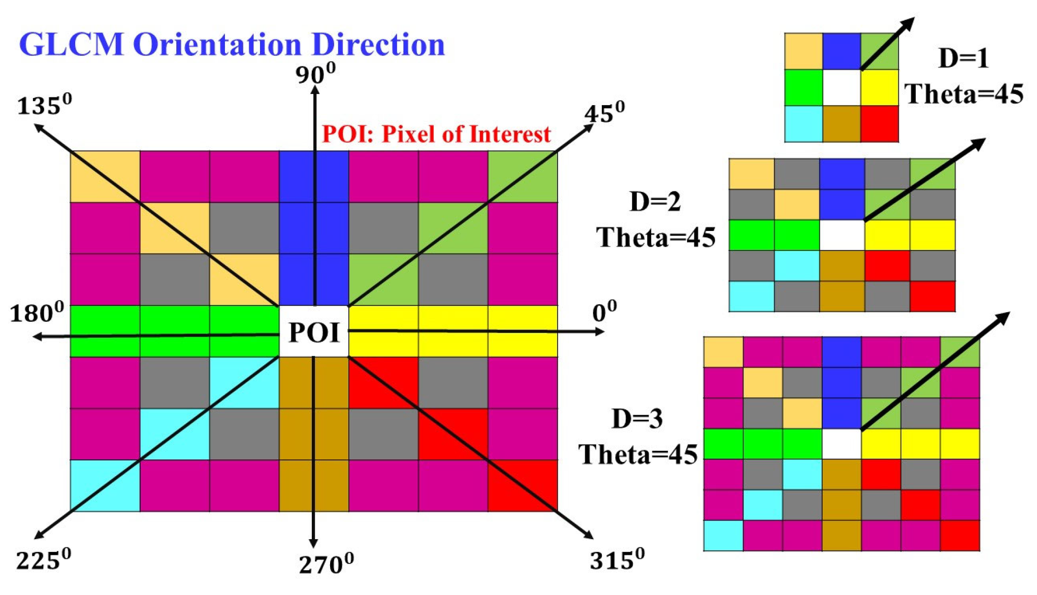
| S. No | Angle | Generalized Offset | Distance D = 1 | Distance D = 2 | Distance D = 3 | Distance D = 4 | Distance D = 5 | Distance D = 6 | Distance D = 7 | Distance D = 8 |
|---|---|---|---|---|---|---|---|---|---|---|
| 1 | ||||||||||
| 2 | ||||||||||
| 3 | ||||||||||
| 4 | ||||||||||
| 5 | ||||||||||
| 6 | ||||||||||
| 7 | ||||||||||
| 8 |
| Texture | Direction | Change in Distances GLCM Features: (Con. = Contrast), (Corr. = Correlation) | |||||||
|---|---|---|---|---|---|---|---|---|---|
| GLCM Visual Features | Angle (Degree) | D = 1 | D = 2 | D = 3 | D = 4 | D = 5 | D = 6 | D = 7 | D = 8 |
| Con. | 0.0619 | 0.1130 | 0.1558 | 0.1945 | 0.2319 | 0.2693 | 0.3080 | 0.3483 | |
| Corr. | 0.9936 | 0.9883 | 0.9838 | 0.9798 | 0.9759 | 0.9721 | 0.9681 | 0.9639 | |
| ASM | 0.1199 | 0.1089 | 0.1010 | 0.0948 | 0.0896 | 0.0851 | 0.0812 | 0.0778 | |
| IDM | 0.9691 | 0.9438 | 0.9234 | 0.9058 | 0.8895 | 0.8743 | 0.8597 | 0.8458 | |
| Con. | 0.0890 | 0.1552 | 0.2125 | 0.2655 | 0.3164 | 0.3673 | 0.4202 | 0.4759 | |
| Corr. | 0.9907 | 0.9839 | 0.9779 | 0.9724 | 0.9672 | 0.9619 | 0.9565 | 0.9507 | |
| ASM | 0.1141 | 0.1019 | 0.0936 | 0.0870 | 0.0817 | 0.0773 | 0.0734 | 0.0701 | |
| IDM | 0.9557 | 0.9251 | 0.9012 | 0.8801 | 0.8613 | 0.8437 | 0.8269 | 0.8110 | |
| Con. | 0.0671 | 0.1216 | 0.1663 | 0.2048 | 0.2391 | 0.2741 | 0.3030 | 0.3349 | |
| Corr. | 0.9930 | 0.9873 | 0.9827 | 0.9787 | 0.9751 | 0.9718 | 0.9685 | 0.9652 | |
| ASM | 0.1192 | 0.1086 | 0.1016 | 0.0964 | 0.0921 | 0.0885 | 0.0853 | 0.0824 | |
| IDM | 0.9666 | 0.9411 | 0.9225 | 0.9075 | 0.8944 | 0.8824 | 0.8712 | 0.8605 | |
| Con. | 0.0934 | 0.1634 | 0.2224 | 0.2762 | 0.3291 | 0.3830 | 0.4395 | 0.4980 | |
| Corr. | 0.9903 | 0.9830 | 0.9768 | 0.9712 | 0.9657 | 0.9601 | 0.9542 | 0.9481 | |
| ASM | 0.1133 | 0.1009 | 0.0926 | 0.0863 | 0.0810 | 0.0765 | 0.0726 | 0.0693 | |
| IDM | 0.9535 | 0.9217 | 0.8975 | 0.8766 | 0.8573 | 0.8392 | 0.8218 | 0.8056 | |
| Texture | Direction | Change in Distances GLCM Features: (Con. = Contrast), (Corr. = Correlation) | |||||||
|---|---|---|---|---|---|---|---|---|---|
| GLCM Visual Features | Angle (Degree) | D = 1 | D = 2 | D = 3 | D = 4 | D = 5 | D = 6 | D = 7 | D = 8 |
| Con. | 0.0730 | 0.1317 | 0.1828 | 0.2308 | 0.2797 | 0.3309 | 0.3843 | 0.4402 | |
| Corr. | 0.9918 | 0.9852 | 0.9795 | 0.9741 | 0.9686 | 0.9628 | 0.9568 | 0.9505 | |
| ASM | 0.1427 | 0.1305 | 0.1220 | 0.1156 | 0.1100 | 0.1050 | 0.1005 | 0.0963 | |
| IDM | 0.9635 | 0.9352 | 0.9133 | 0.8951 | 0.8786 | 0.8630 | 0.8484 | 0.8344 | |
| Con. | 0.1057 | 0.1885 | 0.2613 | 0.3327 | 0.4071 | 0.4849 | 0.5663 | 0.6518 | |
| Corr. | 0.9881 | 0.9788 | 0.9706 | 0.9625 | 0.9542 | 0.9454 | 0.9362 | 0.9266 | |
| ASM | 0.1368 | 0.1239 | 0.1151 | 0.1079 | 0.1018 | 0.0965 | 0.0917 | 0.0875 | |
| IDM | 0.9477 | 0.9143 | 0.8890 | 0.8665 | 0.8461 | 0.8273 | 0.8097 | 0.7934 | |
| Con. | 0.0771 | 0.1431 | 0.1980 | 0.2443 | 0.2874 | 0.3299 | 0.3731 | 0.4173 | |
| Corr. | 0.9913 | 0.9839 | 0.9777 | 0.9726 | 0.9677 | 0.9630 | 0.9581 | 0.9532 | |
| ASM | 0.1437 | 0.1328 | 0.1257 | 0.1203 | 0.1159 | 0.1120 | 0.1085 | 0.1053 | |
| IDM | 0.9617 | 0.9337 | 0.9139 | 0.8978 | 0.8836 | 0.8703 | 0.8578 | 0.8461 | |
| Con. | 0.1060 | 0.1879 | 0.2568 | 0.3229 | 0.3897 | 0.4587 | 0.5309 | 0.6060 | |
| Corr. | 0.9881 | 0.9789 | 0.9712 | 0.9638 | 0.9563 | 0.9486 | 0.9406 | 0.9322 | |
| ASM | 0.1368 | 0.1236 | 0.1150 | 0.1082 | 0.1024 | 0.0974 | 0.0931 | 0.0891 | |
| IDM | 0.9477 | 0.9138 | 0.8888 | 0.8672 | 0.8478 | 0.8301 | 0.8140 | 0.7992 | |
| Texture | Direction | Change in Distances GLCM Features: (Con. = Contrast), (Corr. = Correlation) | |||||||
|---|---|---|---|---|---|---|---|---|---|
| GLCM Visual Features | Angle (Degree) | D = 1 | D = 2 | D = 3 | D = 4 | D = 5 | D = 6 | D = 7 | D = 8 |
| Con. | 0.0795 | 0.1484 | 0.2106 | 0.2702 | 0.3321 | 0.3977 | 0.4681 | 0.5431 | |
| Corr. | 0.9902 | 0.9816 | 0.9738 | 0.9663 | 0.9584 | 0.9501 | 0.9412 | 0.9316 | |
| ASM | 0.1301 | 0.1150 | 0.1044 | 0.0960 | 0.0891 | 0.0832 | 0.0782 | 0.0738 | |
| IDM | 0.9604 | 0.9286 | 0.9030 | 0.8808 | 0.8605 | 0.8418 | 0.8244 | 0.8082 | |
| Con. | 0.1099 | 0.1958 | 0.2759 | 0.3562 | 0.4396 | 0.5278 | 0.6226 | 0.7234 | |
| Corr. | 0.9864 | 0.9756 | 0.9654 | 0.9552 | 0.9445 | 0.9331 | 0.9207 | 0.9075 | |
| ASM | 0.1235 | 0.1074 | 0.0963 | 0.0876 | 0.0806 | 0.0749 | 0.0700 | 0.0659 | |
| IDM | 0.9454 | 0.9073 | 0.8766 | 0.8493 | 0.8247 | 0.8026 | 0.7823 | 0.7638 | |
| Con. | 0.0744 | 0.1318 | 0.1812 | 0.2271 | 0.2706 | 0.3134 | 0.3557 | 0.3996 | |
| Corr. | 0.9908 | 0.9837 | 0.9775 | 0.9718 | 0.9663 | 0.9610 | 0.9557 | 0.9501 | |
| ASM | 0.1323 | 0.1198 | 0.1113 | 0.1047 | 0.0993 | 0.0946 | 0.0907 | 0.0872 | |
| IDM | 0.9628 | 0.9350 | 0.9136 | 0.8953 | 0.8790 | 0.8639 | 0.8502 | 0.8372 | |
| Con. | 0.1086 | 0.1940 | 0.2730 | 0.3513 | 0.4317 | 0.5169 | 0.6080 | 0.7039 | |
| Corr. | 0.9865 | 0.9758 | 0.9658 | 0.9558 | 0.9455 | 0.9345 | 0.9227 | 0.9102 | |
| ASM | 0.1237 | 0.1075 | 0.0965 | 0.0880 | 0.0811 | 0.0754 | 0.0706 | 0.0666 | |
| IDM | 0.9460 | 0.9081 | 0.8776 | 0.8508 | 0.8266 | 0.8041 | 0.7835 | 0.7647 | |
| Texture | Direction | Change in Distance GLCM Features: (Con. = Contrast), (Corr. = Correlation) | |||||||
|---|---|---|---|---|---|---|---|---|---|
| GLCM Visual Features | Angle (Degree) | D = 1 | D = 2 | D = 3 | D = 4 | D = 5 | D = 6 | D = 7 | D = 8 |
| Con. | 0.0607 | 0.1054 | 0.1399 | 0.1696 | 0.1967 | 0.2234 | 0.2498 | 0.2764 | |
| Corr. | 0.9925 | 0.9870 | 0.9827 | 0.9791 | 0.9758 | 0.9725 | 0.9693 | 0.9660 | |
| ASM | 0.1651 | 0.1544 | 0.1471 | 0.1416 | 0.1372 | 0.1333 | 0.1299 | 0.1269 | |
| IDM | 0.9697 | 0.9476 | 0.9308 | 0.9170 | 0.9052 | 0.8940 | 0.8835 | 0.8737 | |
| Con. | 0.0899 | 0.1479 | 0.1938 | 0.2351 | 0.2744 | 0.3126 | 0.3516 | 0.3919 | |
| Corr. | 0.9889 | 0.9817 | 0.9760 | 0.9709 | 0.9661 | 0.9614 | 0.9567 | 0.9517 | |
| ASM | 0.1584 | 0.1466 | 0.1392 | 0.1334 | 0.1286 | 0.1246 | 0.1209 | 0.1176 | |
| IDM | 0.9551 | 0.9278 | 0.9084 | 0.8919 | 0.8774 | 0.8644 | 0.8517 | 0.8397 | |
| Con. | 0.0692 | 0.1193 | 0.1588 | 0.1914 | 0.2202 | 0.2473 | 0.2740 | 0.3006 | |
| Corr. | 0.9914 | 0.9852 | 0.9803 | 0.9763 | 0.9728 | 0.9695 | 0.9662 | 0.9630 | |
| ASM | 0.1636 | 0.1528 | 0.1458 | 0.1409 | 0.1369 | 0.1333 | 0.1301 | 0.1272 | |
| IDM | 0.9655 | 0.9415 | 0.9244 | 0.9113 | 0.9000 | 0.8896 | 0.8797 | 0.8703 | |
| Con. | 0.0892 | 0.1469 | 0.1927 | 0.2334 | 0.2712 | 0.3093 | 0.3469 | 0.3862 | |
| Corr. | 0.9890 | 0.9818 | 0.9762 | 0.9713 | 0.9667 | 0.9621 | 0.9576 | 0.9529 | |
| ASM | 0.1586 | 0.1469 | 0.1395 | 0.1338 | 0.1291 | 0.1249 | 0.1215 | 0.1183 | |
| IDM | 0.9556 | 0.9285 | 0.9092 | 0.8928 | 0.8781 | 0.8642 | 0.8515 | 0.8393 | |
Disclaimer/Publisher’s Note: The statements, opinions and data contained in all publications are solely those of the individual author(s) and contributor(s) and not of MDPI and/or the editor(s). MDPI and/or the editor(s) disclaim responsibility for any injury to people or property resulting from any ideas, methods, instructions or products referred to in the content. |
© 2024 by the authors. Licensee MDPI, Basel, Switzerland. This article is an open access article distributed under the terms and conditions of the Creative Commons Attribution (CC BY) license (https://creativecommons.org/licenses/by/4.0/).
Share and Cite
Shakya, A.K.; Vidyarthi, A. Comprehensive Study of Compression and Texture Integration for Digital Imaging and Communications in Medicine Data Analysis. Technologies 2024, 12, 17. https://0-doi-org.brum.beds.ac.uk/10.3390/technologies12020017
Shakya AK, Vidyarthi A. Comprehensive Study of Compression and Texture Integration for Digital Imaging and Communications in Medicine Data Analysis. Technologies. 2024; 12(2):17. https://0-doi-org.brum.beds.ac.uk/10.3390/technologies12020017
Chicago/Turabian StyleShakya, Amit Kumar, and Anurag Vidyarthi. 2024. "Comprehensive Study of Compression and Texture Integration for Digital Imaging and Communications in Medicine Data Analysis" Technologies 12, no. 2: 17. https://0-doi-org.brum.beds.ac.uk/10.3390/technologies12020017