
Optimized Decentralized Swarm Communication Algorithms for Efficient Task Allocation and Power Consumption in Swarm Robotics

Abstract
:1. Introduction
2. Related Work
2.1. CDTA Stages
- Initialization stage,
- Tuning stage,
- Identification stage,
- Updating stage,
- Stopping stage.
| Algorithm 1 CDTA: main steps executed by a robot | |
|
|
2.2. Hardware Configuration and Applications
3. Methodology
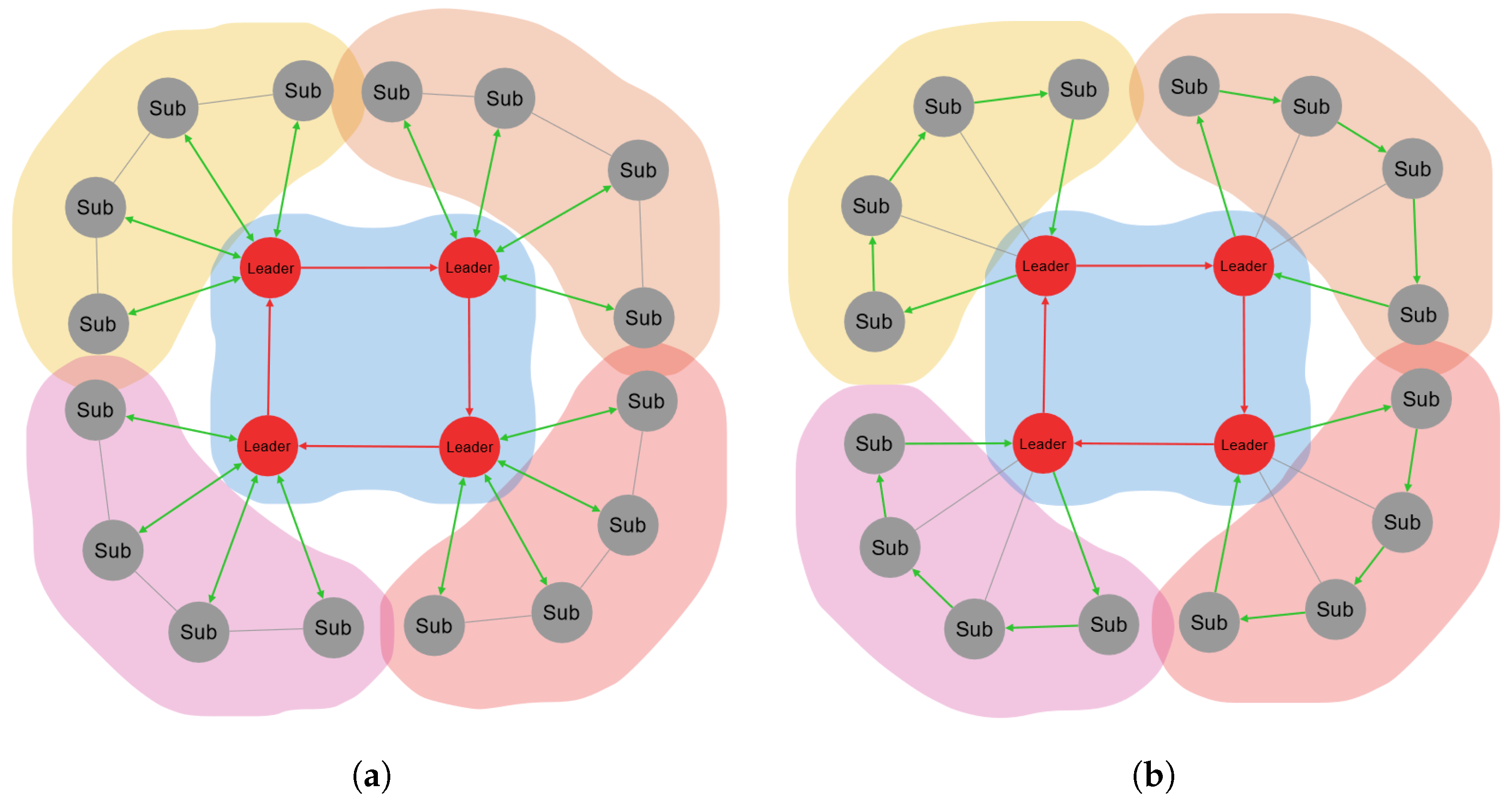
3.1. CDTA-CL and CDTA-DL
- Leader synopsis,
- Leaders’ congregation,
- Result circulation.
3.1.1. Objective Function and Optimization Goal
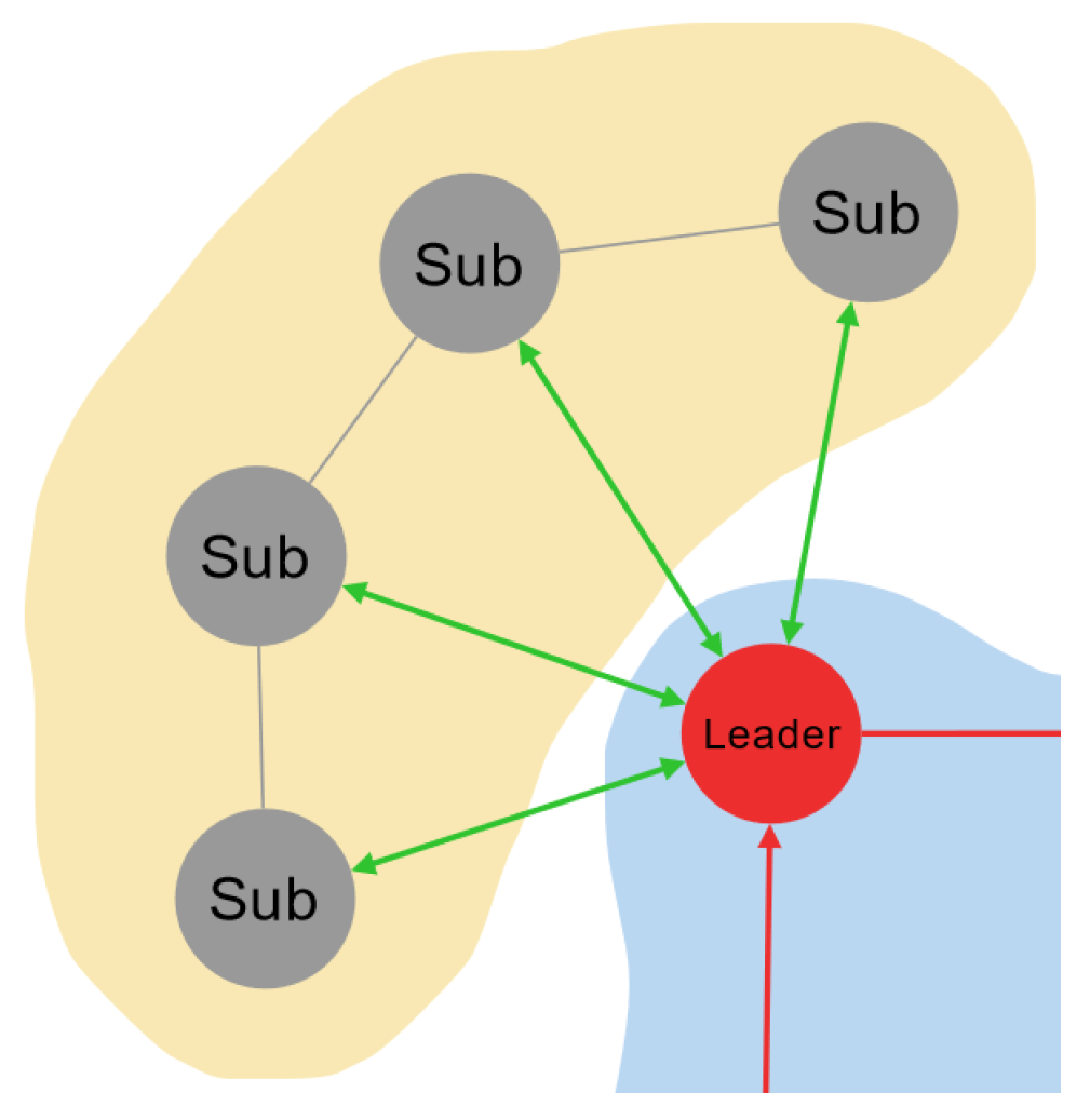
3.1.2. Leader Synopsis
| Algorithm 2 Leader synopsis for CDTA-CL | |
|
|
| Algorithm 3 Leader synopsis for CDTA-DL | |
|
|
3.1.3. Leader Congregation
| Algorithm 4 Leader congregation for CDTA-CL | |
|
|
3.1.4. Result Circulation
- The leader of each cluster calculates the best allocation for the task (Cbest) using information from its subordinates.
- The leaders of all clusters then find the global best allocation (Gbest) among all clusters using the dual loop structure.
- The leaders then ensure that all their subordinates are informed of Gbest, so it becomes swarm-wide knowledge.
- The process follows a centralized or dual loop communication topology, depending on the variation (CDTA-CL or CDTA-DL) being used.
3.2. Self-Organization
- Setting the initial formation of the swarm and its clusters.
- The optimal selection of leader robots for each cluster of the swarm.
- Flexibility and fault tolerance, as follows:
- –
- Interchanging cluster subordinates when they fail or shut down, so that the CDTA-CL and CDTA-DL stages resume normally.
- –
- Re-selection of leader robots for a cluster in case of failure or shutting down.
3.3. Pyswaro Simulation Tool
4. Results
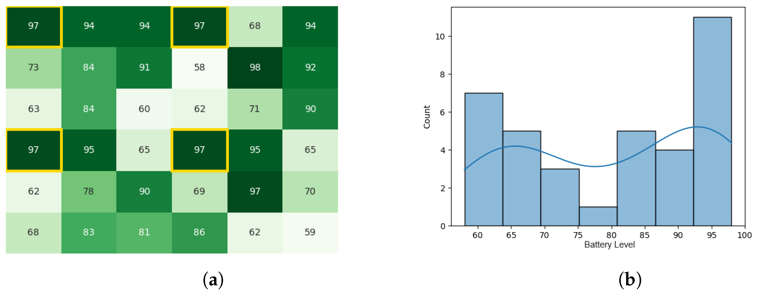
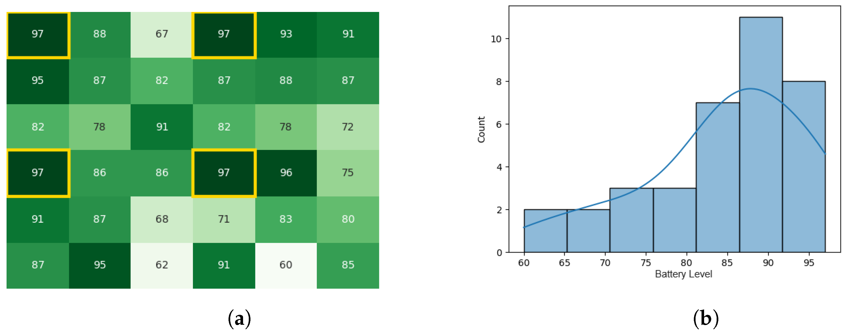
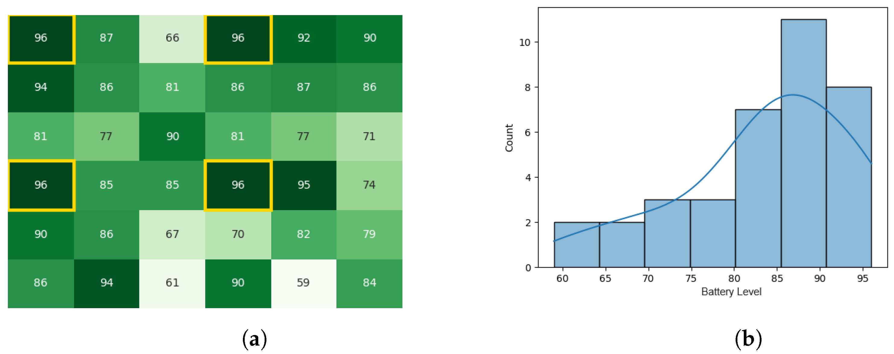
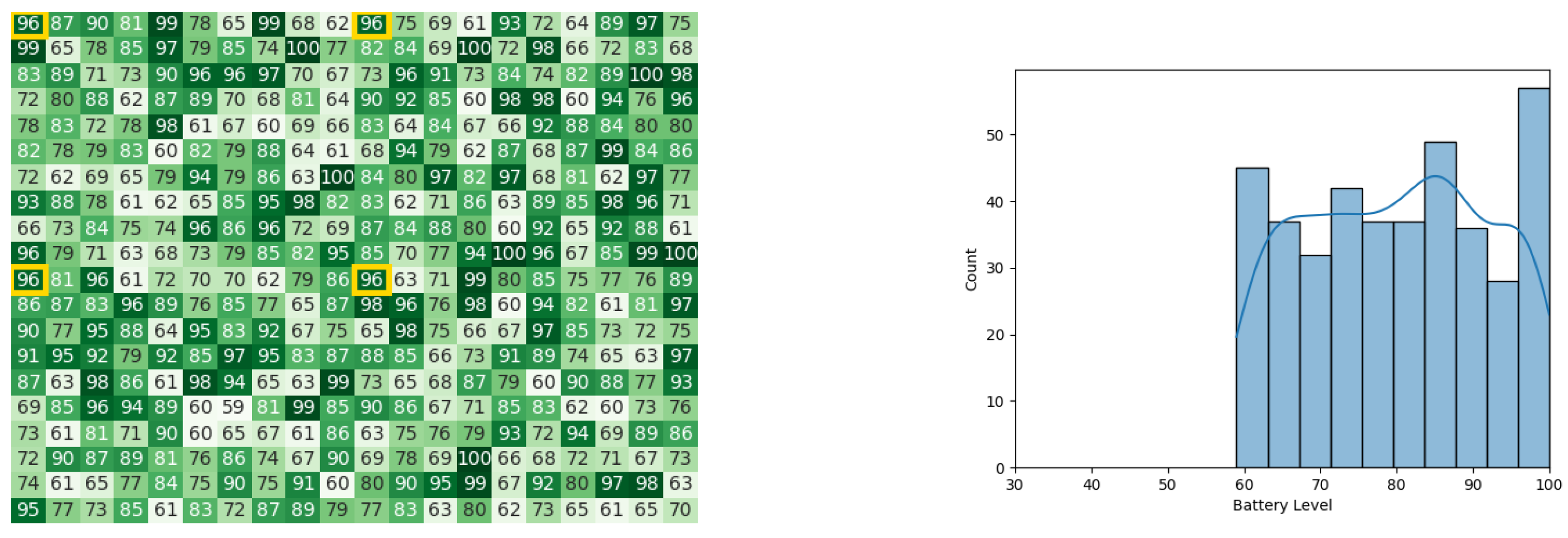
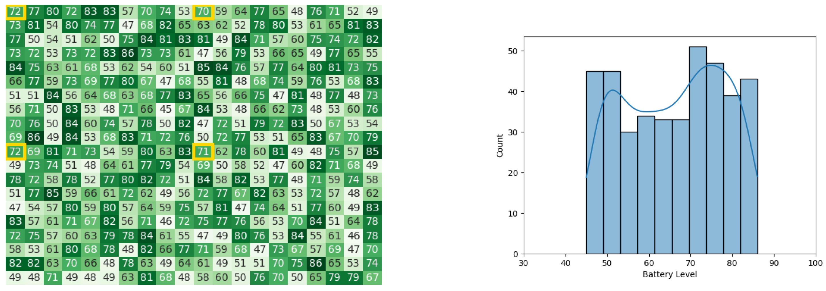
4.1. Experiment 1
- A swarm consisting of 36 robots.
- A minimum initial battery of 60%.
- A maximum initial battery of 100%.
- A minimum operable robot battery of 2%.
- All leaders start with 100% battery.
- All subordinates start with a random battery value between 60% and 100%.
- There are four leaders in the swarm, each leader is responsible for its cluster.
- Each leader has eight subordinates in each of the four clusters.
- Communication delays and battery drainage rates were modeled after the Yanshee robot (see Section 4.3).
4.1.1. Original CDTA Algorithm
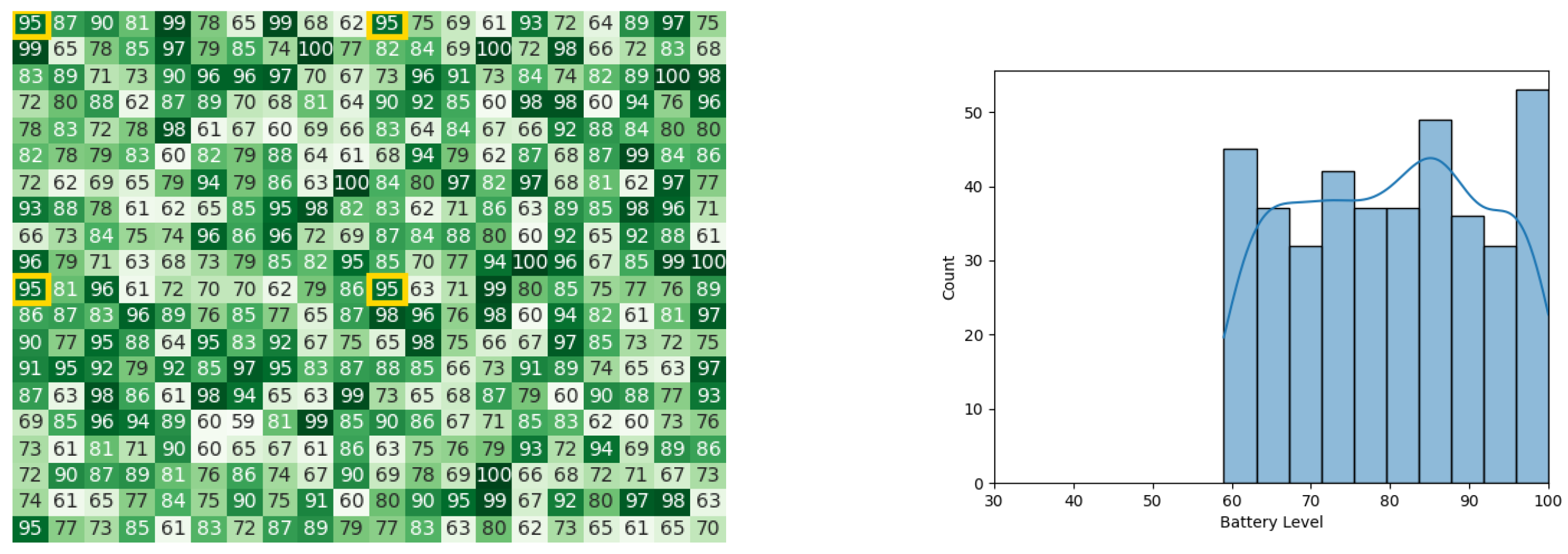
4.1.2. Proposed CDTA-CL Algorithm
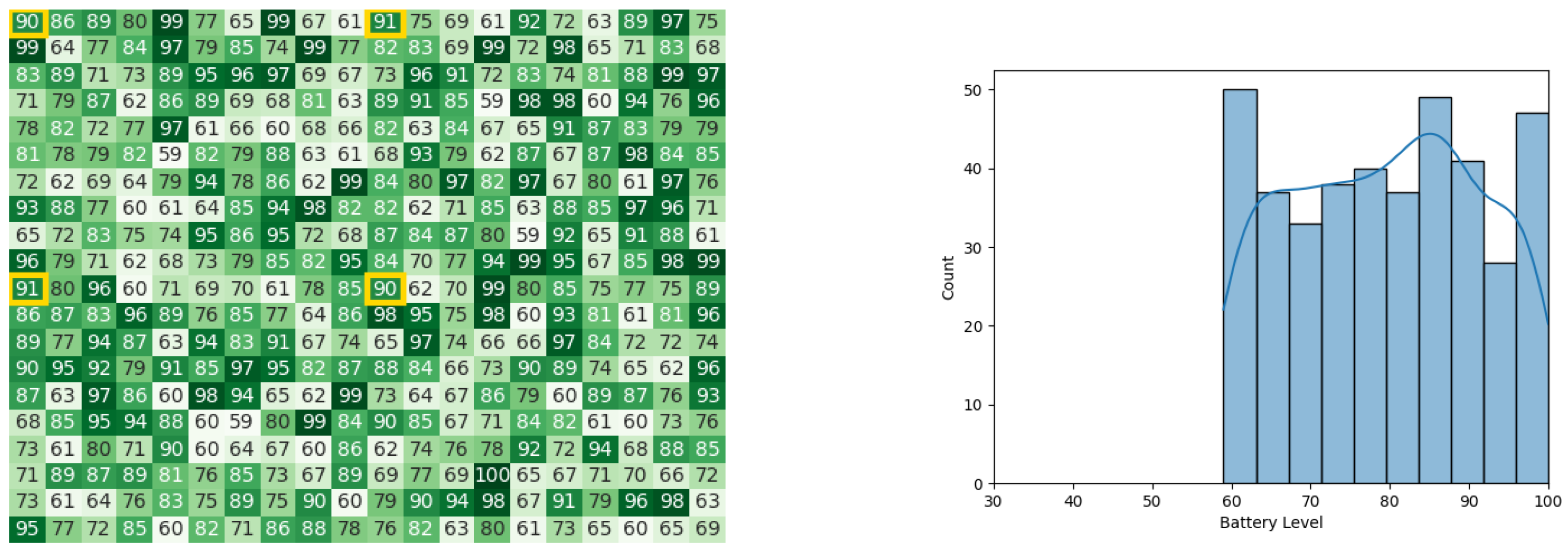
4.1.3. Proposed CDTA-DL Algorithm
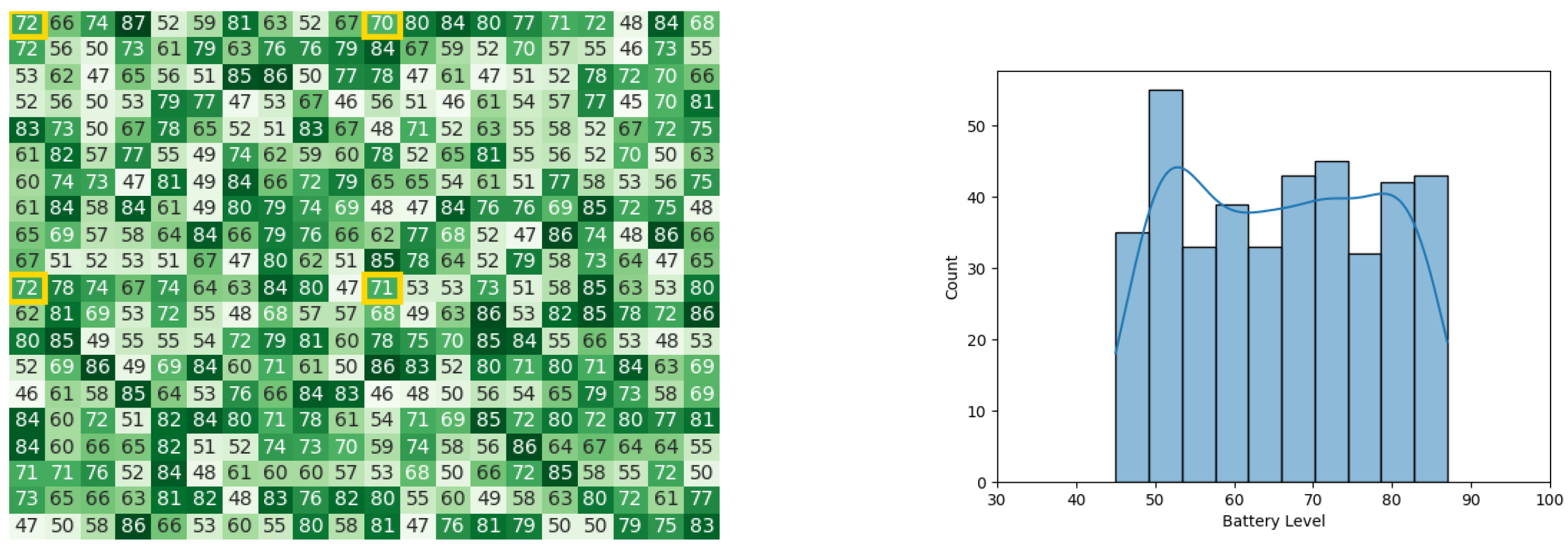
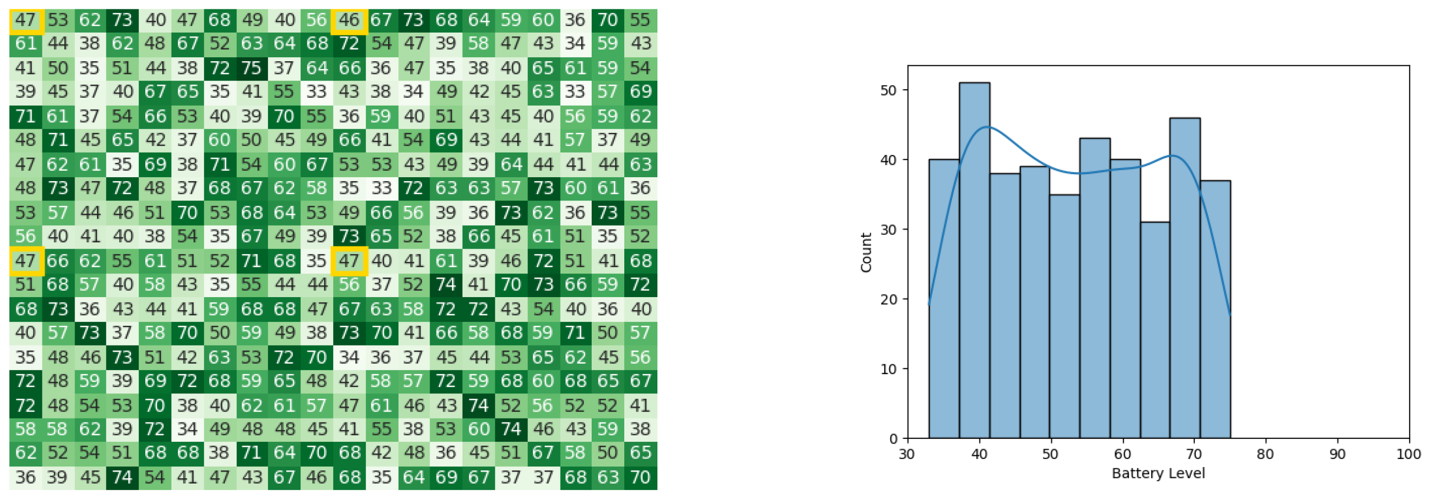
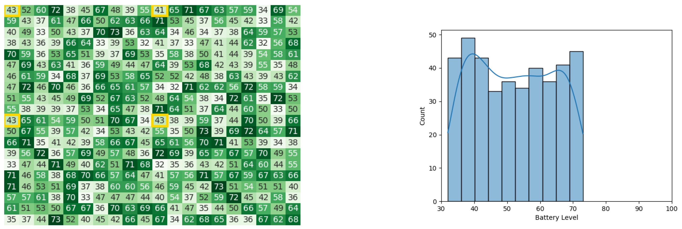
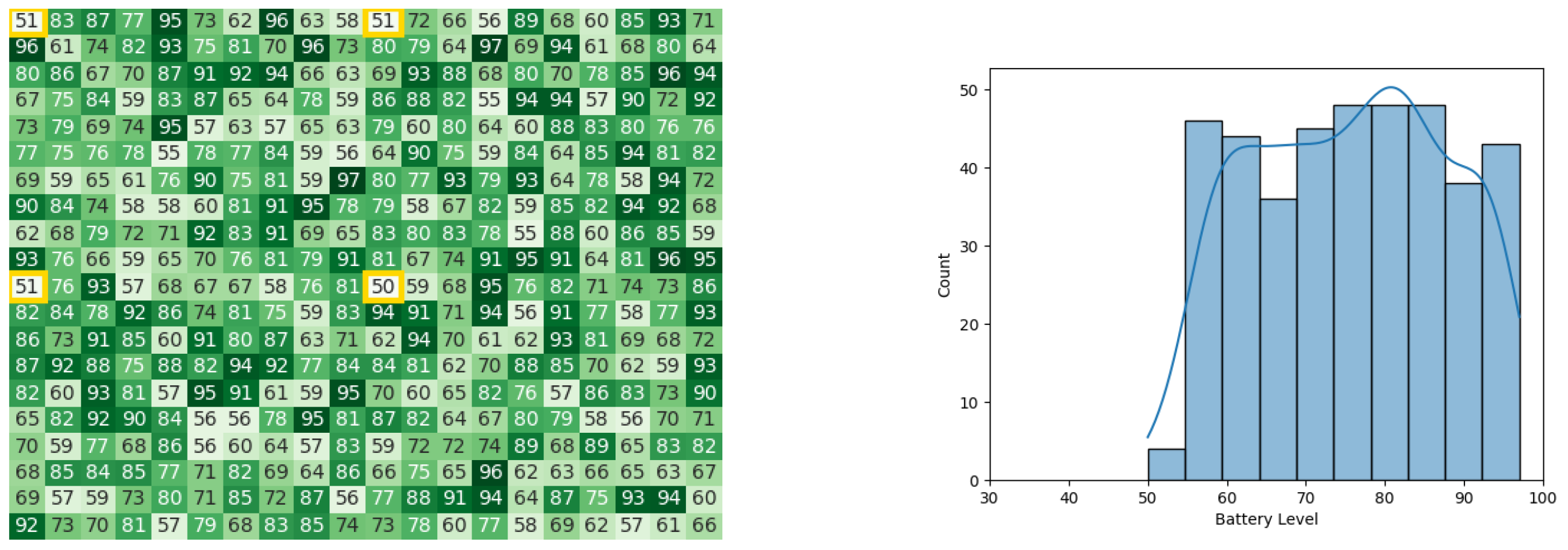
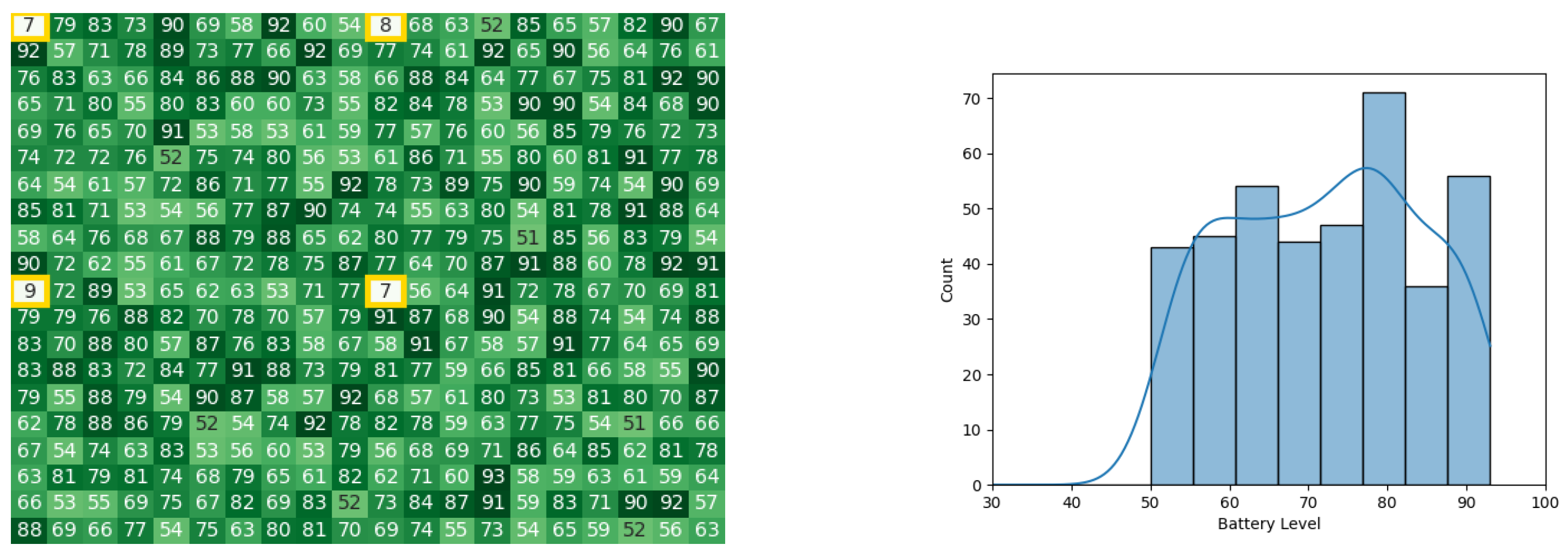
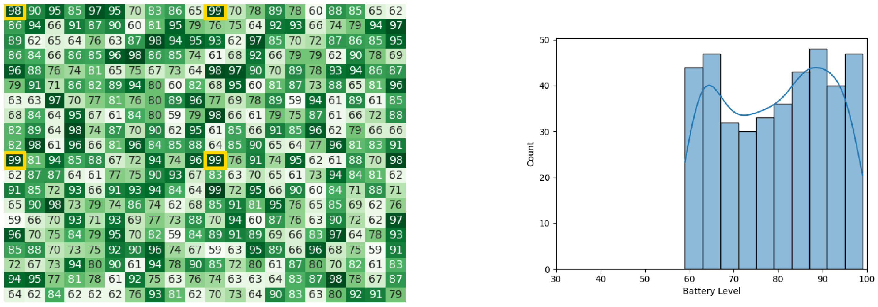
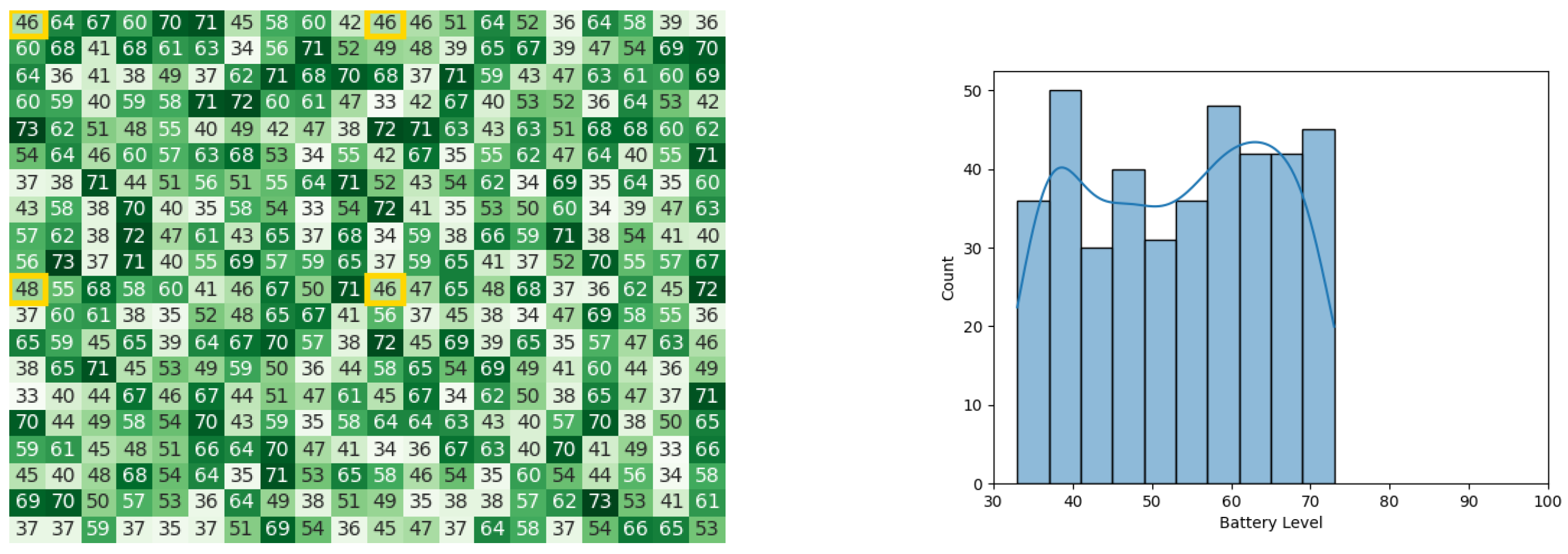
4.2. Experiment 2
- A swarm consisting of 400 robots.
- The swarm operates for 10 iterations.
- A minimum initial battery of 60%.
- A maximum initial battery of 100%.
- A minimum operable robot battery of 2%.
- All leaders start with 100% battery.
- All subordinates start with a random battery value between 60% and 100%.
- There are four leaders in the swarm, each leader is responsible for its cluster.
- Each leader has 99 subordinates in each of the four clusters.
- Communication delays and battery drainage rates were modeled after the Yanshee robot (see Section 4.3).
4.2.1. Original CDTA Algorithm
4.2.2. Proposed CDTA-CL Algorithm
4.2.3. Proposed CDTA-DL Algorithm
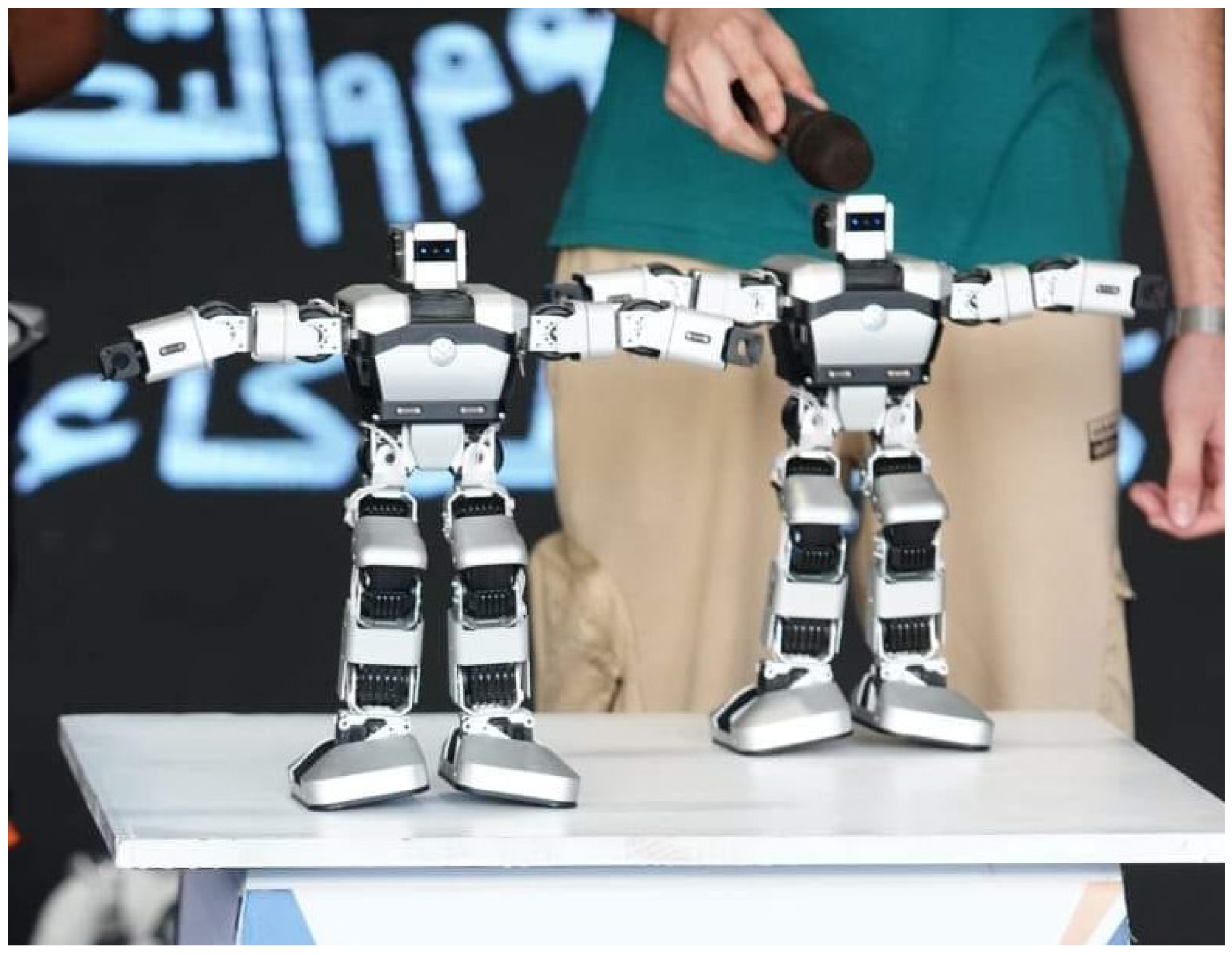
4.3. Testing on Yanshee
- One cluster with one leader and four subordinates.
- Two clusters where one cluster has one leader and two subordinates, while the other has one leader and one subordinate.
4.4. Calculating the Optimal Number of Leaders in CDTA-CL and CDTA-DL
- No battery drainage occurs.
- No communication timeouts occur.
- All leaders have an equal number of subordinates.
- Communication delay was set to 1 ms.
5. Discussion
5.1. Experiment 1
5.2. Experiment 2
6. Conclusion and Future Work
Author Contributions
Funding
Institutional Review Board Statement
Informed Consent Statement
Data Availability Statement
Conflicts of Interest
Abbreviations
| ABC | Artificial Bee Colony |
| ACO | Ant Colony Optimizer |
| CDTA | Clustered Dynamic Task Allocation |
| CDTA-CL | Clustered Dynamic Task Allocation–Centralized Loop |
| CDTA-DL | Clustered Dynamic Task Allocation–Dual Loop |
| DBA | Distributed Bee Algorithm |
| DTA | Dynamic Task Allocation |
| GDTA | Global Dynamic Task Allocation |
| PSO | Particle Swarm Optimization |
| SO | Self-Organization |
References
- Alyassi, R.; Khonji, M.; Karapetyan, A.; Chau, S.C.K.; Elbassioni, K.; Tseng, C.M. Autonomous recharging and flight mission planning for battery-operated autonomous drones. IEEE Trans. Autom. Sci. Eng. 2022, 20, 1034–1046. [Google Scholar] [CrossRef]
- Campion, M.; Ranganathan, P.; Faruque, S. UAV swarm communication and control architectures: A review. J. Unmanned Veh. Syst. 2018, 7, 93–106. [Google Scholar] [CrossRef]
- Khatab, E.; Onsy, A.; Abouelfarag, A. Evaluation of 3D Vulnerable Objects’ Detection Using a Multi-Sensors System for Autonomous Vehicles. Sensors 2022, 22, 1663. [Google Scholar] [CrossRef]
- Ardiny, H.; Witwicki, S.; Mondada, F. Construction automation with autonomous mobile robots: A review. In Proceedings of the 2015 3rd RSI International Conference on Robotics and Mechatronics (ICROM), Tehran, Iran, 7–9 October 2015; IEEE: Piscataway, NJ, USA, 2015; pp. 418–424. [Google Scholar]
- Pang, Z.; Yang, G.; Khedri, R.; Zhang, Y.T. Introduction to the Special Section: Convergence of Automation Technology, Biomedical Engineering, and Health Informatics Toward the Healthcare 4.0. IEEE Rev. Biomed. Eng. 2018, 11, 249–259. [Google Scholar] [CrossRef]
- Rowe, O.S.P. Computer-assisted robotic system for autonomous unicompartmental knee arthroplasty. Alex. Eng. J. 2023, 70, 441–451. [Google Scholar] [CrossRef]
- Albiero, D.; Garcia, A.P.; Umezu, C.K.; de Paulo, R.L. Swarm Robots in Agriculture. arXiv 2021, arXiv:2103.06732. [Google Scholar]
- Kovalev, D.; Salim, A.; Richtárik, P. Optimal and practical algorithms for smooth and strongly convex decentralized optimization. Adv. Neural Inf. Process. Syst. 2020, 33, 18342–18352. [Google Scholar]
- Miyazaki, R.; Murase, T. Centralized Route Control for Expanding Coverage by Wireless LAN with Many Vehicle APs. In Proceedings of the 2021 IEEE 11th Annual Computing and Communication Workshop and Conference (CCWC), Las Vegas, NV, USA, 27–30 January 2021; IEEE: Piscataway, NJ, USA, 2021; pp. 0399–0404. [Google Scholar]
- Maeterlinck, M. The Life of the White Ant; George Allen and Unwin: Crows Nest, NSW, Australia, 1927. [Google Scholar]
- Hölldobler, B.; Wilson, E.O. The Ants; Harvard University Press: Cambridge, MA, USA, 1990. [Google Scholar]
- Zhu, A.; Dai, T.; Xu, G.; Pauwels, P.; de Vries, B.; Fang, M. Deep reinforcement learning for real-time assembly planning in robot-based prefabricated construction. IEEE Trans. Autom. Sci. Eng. 2023, 20, 1515–1526. [Google Scholar] [CrossRef]
- Kehoe, B.; Patil, S.; Abbeel, P.; Goldberg, K. A survey of research on cloud robotics and automation. IEEE Trans. Autom. Sci. Eng. 2015, 12, 398–409. [Google Scholar] [CrossRef]
- Gaber, I.M.; Shalash, O.; Hamad, M.S. Optimized Inter-Turn Short Circuit Fault Diagnosis for Induction Motors using Neural Networks with LeLeRU. In Proceedings of the 2023 IEEE Conference on Power Electronics and Renewable Energy (CPERE), Luxor, Egypt, 9–21 February 2023; IEEE: Piscataway, NJ, USA, 2023; pp. 1–5. [Google Scholar]
- Issa, R.; Badr, M.M.; Shalash, O.; Othman, A.A.; Hamdan, E.; Hamad, M.S.; Abdel-Khalik, A.S.; Ahmed, S.; Imam, S.M. A Data-Driven Digital Twin of Electric Vehicle Li-Ion Battery State-of-Charge Estimation Enabled by Driving Behavior Application Programming Interfaces. Batteries 2023, 9, 521. [Google Scholar] [CrossRef]
- Khatab, E.; Onsy, A.; Varley, M.; Abouelfarag, A. A Lightweight Network for Real-Time Rain Streaks and Rain Accumulation Removal from Single Images Captured by AVs. Appl. Sci. 2022, 13, 219. [Google Scholar] [CrossRef]
- Nicolis, G. Self-organization in nonequilibrium systems. In Dissipative Structures to Order through Fluctuations; Springer: Dordrecht, The Netherlands, 1977; pp. 339–426. [Google Scholar]
- Del Valle, Y.; Venayagamoorthy, G.K.; Mohagheghi, S.; Hernandez, J.C.; Harley, R.G. Particle swarm optimization: Basic concepts, variants and applications in power systems. IEEE Trans. Evol. Comput. 2008, 12, 171–195. [Google Scholar] [CrossRef]
- McMahon, J.; Plaku, E. Autonomous Data Collection With Dynamic Goals and Communication Constraints for Marine Vehicles. IEEE Trans. Autom. Sci. Eng. 2022, 20, 1607–1620. [Google Scholar] [CrossRef]
- Candea, C.; Hu, H.; Iocchi, L.; Nardi, D.; Piaggio, M. Coordination in multi-agent RoboCup teams. Robot. Auton. Syst. 2001, 36, 67–86. [Google Scholar] [CrossRef]
- Brambilla, M.; Ferrante, E.; Birattari, M.; Dorigo, M. Swarm robotics: A review from the swarm engineering perspective. Swarm Intell. 2013, 7, 1–41. [Google Scholar] [CrossRef]
- Hu, W.; Yen, G.G. Adaptive multiobjective particle swarm optimization based on parallel cell coordinate system. IEEE Trans. Evol. Comput. 2013, 19, 1–18. [Google Scholar]
- Bonyadi, M.R. A theoretical guideline for designing an effective adaptive particle swarm. IEEE Trans. Evol. Comput. 2019, 24, 57–68. [Google Scholar] [CrossRef]
- Zhang, Y.; Wang, Y.H.; Gong, D.W.; Sun, X.Y. Clustering-guided particle swarm feature selection algorithm for high-dimensional imbalanced data with missing values. IEEE Trans. Evol. Comput. 2021, 26, 616–630. [Google Scholar] [CrossRef]
- Li, R.; Xiao, Y.; Yang, P.; Tang, W.; Wu, M.; Gao, Y. UAV-aided two-way relaying for wireless communications of intelligent robot swarms. IEEE Access 2020, 8, 56141–56150. [Google Scholar] [CrossRef]
- Sun, Y.; Cai, Z.; Guo, C.; Ma, G.; Zhang, Z.; Wang, H.; Liu, J.; Kang, Y.; Yang, J. Collaborative Dynamic Task Allocation With Demand Response in Cloud-Assisted Multiedge System for Smart Grids. IEEE Internet Things J. 2021, 9, 3112–3124. [Google Scholar] [CrossRef]
- Yang, J.; Ni, J.; Xi, M.; Wen, J.; Li, Y. Intelligent path planning of underwater robot based on reinforcement learning. IEEE Trans. Autom. Sci. Eng. 2022, 20, 1983–1996. [Google Scholar] [CrossRef]
- Camazine, S.; Deneubourg, J.L.; Franks, N.; Sneyd, J.; Theraulaz, G.; Bonabeau, E. Self-Organization in Biological Systems; Princeton Studies in Complexity; Princeton University Press: Princeton, NJ, USA, 2001. [Google Scholar]
- Bonabeau, E.; Theraulaz, G.; Dorigo, M.; Theraulaz, G.; Marco, D.d.R.D.F. Swarm Intelligence: From Natural to Artificial Systems; Number 1; Oxford University Press: Oxford, UK, 1999. [Google Scholar]
- Groß, R.; Bonani, M.; Mondada, F.; Dorigo, M. Autonomous self-assembly in swarm-bots. IEEE Trans. Robot. 2006, 22, 1115–1130. [Google Scholar]
- Pimenta, L.C.; Pereira, G.A.; Michael, N.; Mesquita, R.C.; Bosque, M.M.; Chaimowicz, L.; Kumar, V. Swarm coordination based on smoothed particle hydrodynamics technique. IEEE Trans. Robot. 2013, 29, 383–399. [Google Scholar] [CrossRef]
- Liu, D.; Dou, L.; Zhang, R.; Zhang, X.; Zong, Q. Multi-Agent Reinforcement Learning-Based Coordinated Dynamic Task Allocation for Heterogenous UAVs. IEEE Trans. Veh. Technol. 2022, 72, 4372–4383. [Google Scholar] [CrossRef]
- Pugh, J.; Martinoli, A. Parallel learning in heterogeneous multi-robot swarms. In Proceedings of the 2007 IEEE Congress on Evolutionary Computation, Singapore, 25–28 September 2007; pp. 3839–3846. [Google Scholar]
- Chung, S.J.; Paranjape, A.A.; Dames, P.; Shen, S.; Kumar, V. A survey on aerial swarm robotics. IEEE Trans. Robot. 2018, 34, 837–855. [Google Scholar] [CrossRef]
- Yang, L.; Yu, J.; Yang, S.; Wang, B.; Nelson, B.J.; Zhang, L. A survey on swarm microrobotics. IEEE Trans. Robot. 2021, 38, 1531–1551. [Google Scholar] [CrossRef]
- Shami, T.M.; El-Saleh, A.A.; Alswaitti, M.; Al-Tashi, Q.; Summakieh, M.A.; Mirjalili, S. Particle swarm optimization: A comprehensive survey. IEEE Access 2022, 10, 10031–10061. [Google Scholar] [CrossRef]
- Rossides, G.; Metcalfe, B.; Hunter, A. Particle Swarm Optimization—An Adaptation for the Control of Robotic Swarms. Robotics 2021, 10, 58. [Google Scholar] [CrossRef]
- Yingying, D.; Yan, H.; Jingping, J. Multi-robot cooperation method based on the ant algorithm. In Proceedings of the Proceedings of the 2003 IEEE Swarm Intelligence Symposium. SIS’03 (Cat. No. 03EX706), Indianapolis, IN, USA, 26 April 2003; pp. 14–18. [Google Scholar]
- Zhang, D.; Xie, G.; Yu, J.; Wang, L. Adaptive task assignment for multiple mobile robots via swarm intelligence approach. Robot. Auton. Syst. 2007, 55, 572–588. [Google Scholar] [CrossRef]
- Jevtic, A.; Gutiérrez, A.; Andina, D.; Jamshidi, M. Distributed bees algorithm for task allocation in swarm of robots. IEEE Syst. J. 2011, 6, 296–304. [Google Scholar] [CrossRef]
- Jevtić, A.; Gutiérrez, A. Distributed bees algorithm parameters optimization for a cost efficient target allocation in swarms of robots. Sensors 2011, 11, 10880–10893. [Google Scholar] [CrossRef] [PubMed]
- Tkach, I.; Jevtić, A.; Nof, S.Y.; Edan, Y. A modified distributed bees algorithm for multi-sensor task allocation. Sensors 2018, 18, 759. [Google Scholar] [CrossRef] [PubMed]
- Lee, W.; Kim, D. Adaptive approach to regulate task distribution in swarm robotic systems. Swarm Evol. Comput. 2019, 44, 1108–1118. [Google Scholar] [CrossRef]
- Ji, J.; Guo, Y.; Gong, D.; Shen, X. Evolutionary multi-task allocation for mobile crowdsensing with limited resource. Swarm Evol. Comput. 2021, 63, 100872. [Google Scholar] [CrossRef]
- Karaboga, D.; Okdem, S.; Ozturk, C. Cluster based wireless sensor network routing using artificial bee colony algorithm. Wirel. Networks 2012, 18, 847–860. [Google Scholar] [CrossRef]
- Lerman, K.; Jones, C.; Galstyan, A.; Matarić, M.J. Analysis of dynamic task allocation in multi-robot systems. Int. J. Robot. Res. 2006, 25, 225–241. [Google Scholar] [CrossRef]
- Eberhart, R.; Kennedy, J. A new optimizer using particle swarm theory. In Proceedings of the MHS’95. Proceedings of the Sixth International Symposium on Micro Machine and Human Science, Nagoya, Japan, 4–6 October 1995; pp. 39–43. [Google Scholar]
- Nedjah, N.; de Mendonça, R.M.; de Macedo Mourelle, L. PSO-based distributed algorithm for dynamic task allocation in a robotic swarm. Procedia Comput. Sci. 2015, 51, 326–335. [Google Scholar] [CrossRef]
- Nedjah, N.; Ribeiro, L.M.; de Macedo Mourelle, L. Communication optimization for efficient dynamic task allocation in swarm robotics. Appl. Soft Comput. 2021, 105, 107297. [Google Scholar] [CrossRef]
- Sun, Y.; Li, W.; Ruan, J. Generalized outer synchronization between complex dynamical networks with time delay and noise perturbation. Commun. Nonlinear Sci. Numer. Simul. 2013, 18, 989–998. [Google Scholar] [CrossRef]
- Arellano-Delgado, A.; López-Gutiérrez, R.M.; Murillo-Escobar, M.Á.; Posadas-Castillo, C. Master–Slave Outer Synchronization in Different Inner–Outer Coupling Network Topologies. Entropy 2023, 25, 707. [Google Scholar] [CrossRef]
- Shi, Y.; RC, E. A Modified Particle Swarm Optimizer. In Proceedings of the 1998 IEEE International Conference on Evolutionary Computation Proceedings. IEEE World Congress on Computational Intelligence (Cat. No.98TH8360), Anchorage, AK, USA, 4–9 May 1998; pp. 69–73. [Google Scholar] [CrossRef]
- Atmel. ATmega 2560 Data Sheet. Techreport, 1600 Technology Drive San Jose, CA 95110 United States, 2022. Available online: https://ww1.microchip.com/downloads/en/devicedoc/atmel-2549-8-bit-avr-microcontroller-atmega640-1280-1281-2560-2561_datasheet.pdf (accessed on 10 March 2023).
- Semiconductors, N. Preliminary Product Specification V1. Technical Report. 2022. Available online: https://www.sparkfun.com/datasheets/Components/SMD/nRF24L01Pluss_Preliminary_Product_Specification_v1_0.pdf (accessed on 10 March 2023).
- Vaezinejad, S.; Marandi, S.M.; Salajegheh, E. A Hybrid of Artificial Neural Networks and Particle Swarm Optimization Algorithm for Inverse Modeling of Leakage in Earth Dams. Civ. Eng. J. 2019, 5, 2041–2057. [Google Scholar] [CrossRef]
- de Pinho Pinheiro, C.A.; Nedjah, N.; de Macedo Mourelle, L. Detection and classification of pulmonary nodules using deep learning and swarm intelligence. Multimed. Tools Appl. 2020, 79, 15437–15465. [Google Scholar] [CrossRef]
- Ramos, J.; Nedjah, N.; Mourelle, L.; Gupta, B.B. Visual data mining for crowd anomaly detection using artificial bacteria colony. Multimed. Tools Appl. 2018, 77, 17755–17777. [Google Scholar] [CrossRef]
- Tavares, Y.; Nedjah, N.; Mourelle, L. Embedded implementation of template matching using correlation and particle swarm optimisation. Int. J. Bio-Inspired Comput. 2018, 11, 102. [Google Scholar] [CrossRef]
- Qin, B.; Zhang, D.; Tang, S.; Wang, M. Distributed Grouping Cooperative Dynamic Task Assignment Method of UAV Swarm. Appl. Sci. 2022, 12, 2865. [Google Scholar] [CrossRef]
- Yasser, M. Pyswaro. 2022. Available online: https://github.com/MohamedYasser97/pyswaro (accessed on 2 June 2023).
- UBTECH ROBOTICS CORP. Yanshee User Manual; Techreport; UBTECH ROBOTICS CORP: Shenzhen, China, 2018. [Google Scholar]


| Algorithm | Swarm Configuration | Time | Unit |
|---|---|---|---|
| Original CDTA | 1 leader, 4 subordinates | 2.31 | seconds |
| Original CDTA | 2 leaders, 3 subordinates | 2.08 | seconds |
| CDTA-CL Variation | 1 leader, 4 subordinates | 1.076 | seconds |
| CDTA-CL Variation | 2 leaders, 3 subordinates | 0.84 | seconds |
| CDTA-DL Variation | 1 leader, 4 subordinates | 0.577 | seconds |
| CDTA-DL Variation | 2 leaders, 3 subordinates | 0.468 | seconds |
| 32 Robots | 64 Robots | 128 Robots | 256 Robots | 512 Robots | 1024 Robots | 2048 Robots | 4096 Robots | Time | |
|---|---|---|---|---|---|---|---|---|---|
| 1 leader | 0.126 | 0.254 | 0.51 | 1.022 | 2.046 | 4.094 | 8.19 | 16.382 | seconds |
| 2 leaders | 0.064 | 0.128 | 0.256 | 0.512 | 1.024 | 2.048 | 4.096 | 8.192 | seconds |
| 4 leaders | 0.036 | 0.068 | 0.132 | 0.26 | 0.516 | 1.028 | 2.052 | 4.1 | seconds |
| 8 leaders | 0.028 | 0.044 | 0.076 | 0.14 | 0.268 | 0.524 | 1.036 | 2.06 | seconds |
| 16 leaders | 0.036 | 0.044 | 0.06 | 0.092 | 0.156 | 0.284 | 0.54 | 1.052 | seconds |
| 32 leaders | 0.068 | 0.076 | 0.092 | 0.124 | 0.188 | 0.316 | 0.572 | seconds | |
| 64 leaders | 0.132 | 0.14 | 0.156 | 0.188 | 0.252 | 0.38 | seconds | ||
| 128 leaders | 0.26 | 0.268 | 0.284 | 0.316 | 0.38 | seconds | |||
| 256 leaders | 0.516 | 0.524 | 0.54 | 0.572 | seconds | ||||
| 512 leaders | 1.028 | 1.036 | 1.052 | seconds | |||||
| 1024 leaders | 2.052 | 2.06 | seconds | ||||||
| 2048 leaders | 4.1 | seconds |
| 32 Robots | 64 Robots | 128 Robots | 256 Robots | 512 Robots | 1024 Robots | 2048 Robots | 4096 Robots | Time | |
|---|---|---|---|---|---|---|---|---|---|
| 1 leader | 0.066 | 0.13 | 0.258 | 0.514 | 1.026 | 2.05 | 4.098 | 8.194 | seconds |
| 2 leaders | 0.036 | 0.068 | 0.132 | 0.26 | 0.516 | 1.028 | 2.052 | 4.1 | seconds |
| 4 leaders | 0.024 | 0.04 | 0.072 | 0.136 | 0.264 | 0.52 | 1.032 | 2.056 | seconds |
| 8 leaders | 0.024 | 0.032 | 0.048 | 0.08 | 0.144 | 0.272 | 0.528 | 1.04 | seconds |
| 16 leaders | 0.036 | 0.04 | 0.048 | 0.064 | 0.096 | 0.16 | 0.288 | 0.544 | seconds |
| 32 leaders | 0.068 | 0.072 | 0.08 | 0.096 | 0.128 | 0.192 | 0.32 | seconds | |
| 64 leaders | 0.132 | 0.136 | 0.144 | 0.16 | 0.192 | 0.256 | seconds | ||
| 128 leaders | 0.26 | 0.264 | 0.272 | 0.288 | 0.32 | seconds | |||
| 256 leaders | 0.516 | 0.52 | 0.528 | 0.544 | seconds | ||||
| 512 leaders | 1.028 | 1.032 | 1.04 | seconds | |||||
| 1024 leaders | 2.052 | 2.056 | seconds | ||||||
| 2048 leaders | 4.1 | seconds |
| Original CDTA | Proposed CDTA-CL | Proposed CDTA-DL | Unit | |
|---|---|---|---|---|
| Execution Time | 0.333 | 0.152 | 0.08 | Seconds |
| Average Initial Battery Level | 82.36% | 84% | 85.64% | Battery Level |
| Average Final Battery Level | 80.25% | 81.56% | 83.42% | Battery Level |
| Minimum Power Lost by a Single Robot During Operation | 2% | Battery Level | ||
| Maximum Power Lost by a Single Robot During Operation | 3% | 12% | 4% | Battery Level |
| Average Power Loss by Any Robot During Operation | 2.1% | 2.4% | 2.2% | Battery Level |
| Standard Deviation of Battery Power Loss | 0.32% | 1.73% | 0.64% | Battery Level |
| Variance of Battery Power Loss | 0.1 | 3 | 0.41 | (Battery Level)2 |
| Swarm Population | Original CDTA | Proposed CDTA-CL | Proposed CDTA-DL | Unit |
|---|---|---|---|---|
| 36 robots |4 leaders | 0.333 | 0.152 | 0.08 | Seconds |
| 100 robots|4 leaders | 0.909 | 0.408 | 0.208 | Seconds |
| 10,000 robots|4 leaders | 90 | 40 | 20 | Seconds |
| 1,000,000 robots|4 leaders | 2.5 | 1.1 | 0.55 | Hours |
| 100,000,000 robots|4 leaders | 10.4 | 4.6 | 2.3 | Days |
| Original CDTA | Proposed CDTA-CL | Proposed CDTA-DL | Unit | |
|---|---|---|---|---|
| Execution Time | 41.89 | 18.791 | 9.897 | Seconds |
| Average Initial Battery Level | 79.84% | 80.38% | 80.59% | Battery Level |
| Average Final Battery Level | 52.15% | 71.05% | 51.6% | Battery Level |
| Minimum Power Lost by a Single Robot During Operation | 24.75% | 5.2% | 26.32% | Battery Level |
| Maximum Power Lost by a Single Robot During Operation | 58.65% | 98.81% | 58.69% | Battery Level |
| Average Power Loss by Any Robot During Operation | 27.69% | 9.33% | 28.98% | Battery Level |
| Standard Deviation of Battery Power Loss | 3.15% | 8.92% | 3.02% | Battery Level |
| Variance of Battery Power Loss | 9.94 | 79.62 | 9.15 | (Battery Level)2 |
Disclaimer/Publisher’s Note: The statements, opinions and data contained in all publications are solely those of the individual author(s) and contributor(s) and not of MDPI and/or the editor(s). MDPI and/or the editor(s) disclaim responsibility for any injury to people or property resulting from any ideas, methods, instructions or products referred to in the content. |
© 2024 by the authors. Licensee MDPI, Basel, Switzerland. This article is an open access article distributed under the terms and conditions of the Creative Commons Attribution (CC BY) license (https://creativecommons.org/licenses/by/4.0/).
Share and Cite
Yasser, M.; Shalash, O.; Ismail, O. Optimized Decentralized Swarm Communication Algorithms for Efficient Task Allocation and Power Consumption in Swarm Robotics. Robotics 2024, 13, 66. https://0-doi-org.brum.beds.ac.uk/10.3390/robotics13050066
Yasser M, Shalash O, Ismail O. Optimized Decentralized Swarm Communication Algorithms for Efficient Task Allocation and Power Consumption in Swarm Robotics. Robotics. 2024; 13(5):66. https://0-doi-org.brum.beds.ac.uk/10.3390/robotics13050066
Chicago/Turabian StyleYasser, Mohamed, Omar Shalash, and Ossama Ismail. 2024. "Optimized Decentralized Swarm Communication Algorithms for Efficient Task Allocation and Power Consumption in Swarm Robotics" Robotics 13, no. 5: 66. https://0-doi-org.brum.beds.ac.uk/10.3390/robotics13050066