Article

Learning to Execute Timed-Temporal-Logic Navigation Tasks under Input Constraints in Obstacle-Cluttered Environments †

by
Fotios C. Tolis
1,
Panagiotis S. Trakas
1,
Taxiarchis-Foivos Blounas
1,
Christos K. Verginis
2 and
Charalampos P. Bechlioulis
1,3,*
1
Division of Signals and Control Systems, Department of Electrical and Computer Engineering, University of Patras, Rio, 26504 Patras, Greece
2
Division of Signals and Systems, Department of Electrical Engineering, Uppsala University, 752 37 Uppsala, Sweden
3
Athena Research Center, Robotics Institute, Artemidos 6 & Epidavrou, 15125 Marousi, Greece
*
Author to whom correspondence should be addressed.
Verginis, C.K.; Vrohidis, C.; Bechlioulis, C.P.; Kyriakopoulos, K.J.; Dimarogonas, D.V. Reconfigurable motion planning and control in obstacle cluttered environments under timed temporal tasks. In Proceedings of the 2019 International Conference on Robotics and Automation (ICRA), Montreal, QC, Canada, 20–24 May 2019; pp. 951–957.
Submission received: 6 February 2024 / Revised: 29 March 2024 / Accepted: 23 April 2024 / Published: 26 April 2024
(This article belongs to the Special Issue Motion Trajectory Prediction for Mobile Robots)

Abstract

:
This study focuses on addressing the problem of motion planning within workspaces cluttered with obstacles while considering temporal and input constraints. These specifications can encapsulate intricate high-level objectives involving both temporal and spatial constraints. The existing literature lacks the ability to fulfill time specifications while simultaneously managing input-saturation constraints. The proposed approach introduces a hybrid three-component control algorithm designed to learn the safe execution of a high-level specification expressed as a timed temporal logic formula across predefined regions of interest in the workspace. The first component encompasses a motion controller enabling secure navigation within the minimum allowable time interval dictated by input constraints, facilitating the abstraction of the robot’s motion as a timed transition system between regions of interest. The second component utilizes formal verification and convex optimization techniques to derive an optimal high-level timed plan over the mentioned transition system, ensuring adherence to the agent’s specification. However, the necessary navigation times and associated costs among regions are initially unknown. Consequently, the algorithm’s third component iteratively adjusts the transition system and computes new plans as the agent navigates, acquiring updated information about required time intervals and associated navigation costs. The effectiveness of the proposed scheme is demonstrated through both simulation and experimental studies.

1. Introduction

In recent years, there has been a notable research focus on temporal-logic-based motion planning, driven by its automated, correct-by-design control synthesis approach for autonomous robots. Temporal logics provide a powerful framework for articulating planning objectives that go beyond simple point-to-point navigation [1,2,3,4,5,6,7]. The integration of time constraints widens the scope to encompass a broader range of tasks, such as “collect data in region C every 20 s and transfer it to region D at least once every 120 s”. Such capabilities are crucial for autonomous systems operating in dynamic and time-sensitive environments.
Tasks formulated using timed temporal logics such as Metric Temporal Logic (MTL) or Metric Interval Temporal Logic (MITL) [8] necessitate abstracting the robot’s motion into a transition system across predefined regions in the workspace. This abstraction requires implementing suitable feedback controllers to facilitate timed navigation between these regions. Additionally, as robots operate in environments cluttered with obstacles and are subject to input-saturation constraints, designing such controllers becomes highly complex. The duration of navigation within the workspace, accounting for these constraints, cannot be arbitrarily predetermined. These insights showcase the challenge of motion planning under timed temporal tasks and input constraints in obstacle-cluttered environments, which we address in this paper. In particular, hardware constraints inherently impose limitations on actuation capacity in robotic systems. These constraints can significantly degrade the performance of closed-loop systems, resulting in inaccuracies or even instability. Consequently, developing control strategies that effectively handle these actuation constraints holds practical importance and theoretical significance. Nonetheless, it remains a formidable challenge for designers of control systems.

Related Works and Contributions

Numerous works in the literature handle tasks expressed through timed temporal logics, including MTL or MITL [9,10,11,12,13,14,15,16,17,18,19,20]. However, several of these works overlook continuous robot dynamics, either assuming unrestricted robot navigation in a predefined time or assuming obstacle-free environments [11,12,13,15]. Achieving timed navigation in obstacle-cluttered environments is explored in [14] through sampling-based planning but without considering timed temporal logic formulas. Some works, such as [9,16,17,18,21], address obstacle avoidance by partitioning the workspace into cells and utilizing graph-search methods. Nevertheless, these methodologies can be computationally intensive in large workspaces. A manipulation planning framework that employs linear temporal logic (LTL) specifications, enabling the expression of complex tasks, was presented in [22]. The framework tackles computational hurdles through an abstraction method and employs a multi-layered planning structure. However, the planner’s runtime performance deteriorates with an increase in the number of objects and locations and with more complex LTL specifications. The authors of [23] propose an integrated approach combining motion planning and hybrid feedback control to achieve complex MITL missions. In particular, they utilize sampling-based motion planning to find waypoints, compute timestamps for reaching waypoints based on clock zones, and employ Time-Varying Control Barrier Functions for low-level feedback control between waypoints. Additionally, the approaches in [16,17,21] use optimization techniques that yield maximum-velocity controllers, potentially leading to conservative estimates of transition times and unnecessarily high control effort. More recently, the authors of [24] introduced a reactive control scheme, emphasizing its ability to meet LTL specifications while demonstrating resilience to disturbances. The work in [25] presents a formal control framework aimed at achieving temporal logic tasks and addressing challenges arising from conflicts between mission objectives and safety constraints. Additionally, the synthesis of controllers under asynchronous temporal robustness constraints is explored in [26], ensuring resilience against individual time shifts within its sub-trajectories. The work in [27] introduces a robust task and motion planning algorithm, blending dynamic planning and behavior-tree-based control strategies for the reactive TAMP method by employing LTL and motion cost approximation. Notably, most of the related works in the literature (e.g., [9,10,11,13,16,18,19,20,24,25,26,27,28,29]) entirely neglect input-saturation constraints and their defining impact on the evolution of robot dynamics, consequently affecting task satisfaction.
This work introduces a novel control scheme by incorporating input constraints into the motion planning problem under timed temporal task objectives. The proposed algorithm learns to execute a given timed task optimally considering the input constraints. Initially, given predefined regions of interest in an obstacle-cluttered workspace, previous results on closed-loop feedback navigation [30] are utilized to enable safe timed transitions of the robot, which are achieved via a robust controller designed based on the adaptive performance control methodology [31]. This facilitates the abstraction of the robot as a timed transition system over the regions without requiring further refinement of the workspace partition. Unlike our prior work in [10], arbitrary time constraints for each transition are no longer guaranteed due to input limitations. More specifically, these limitations can hinder the completion of each transition in a prespecified time span, and, therefore, the corresponding time constraints can no longer be arbitrarily set. To address this, we employ an iterative learning scheme utilizing formal verification techniques to derive a plan satisfying the untimed specification. The assignment of transition times is then recast as a convex optimization problem. The algorithm considers time violations, recalculating times after each transition by incorporating newly acquired information about the time and control effort required for task completion.
The main contributions of this work are summarized as follows:
  • Contrary to [9,10,11,13,16,18,19,20,24,25,26,27,28,29], the proposed learning algorithm for timed temporal tasks addresses input constraints that inherently lead to plan reconfiguration.
  • We significantly extend the path planner of [30] by considering more generic workspaces, unicycle robot dynamics, and input constraints.
  • The implemented low-level controller guarantees the robot’s safe navigation within workspaces cluttered with obstacles, requiring no prior knowledge of the system or extensive parameter tuning, which facilitates the integration into realistic experimental setups.

2. Preliminaries

In this section, we provide an overview of certain foundational concepts that will be referenced throughout the subsequent discussion.
An atomic proposition is a statement concerning problem variables and parameters that can assume a truth value of either True(⊤) or False (⊥) at a specific time instance.
Definition 1. 
A time sequence t 0 t 1 t 2 [32] constitutes an infinite series of time values t j R 0 , j N 0 , where each value is determined by adding a constant t j , j + 1 R 0 to the preceding one.
Definition 2. 
A timed word w over a finite set of atomic propositions AP consists of an infinite sequence w = ( w 0 , t 0 ) ( w 1 , t 1 ) , , where w 0 , w 1 , w 2 , forms an infinite word over 2 AP and t 0 , t 1 , t 2 , represents a time sequence.
Definition 3. 
A Weighted Transition System (WTS) is a tuple T Π , Π 0 , , AP , L , γ , where Π is a finite set of states, Π 0 Π is a set of initial states, Π × Π is a transition relation, AP is a finite set of atomic propositions, L : Π 2 AP is a labeling function, and  γ : R 0 is a map that assigns a weight to each transition.
Definition 4. 
A timed run of a WTS is an infinite sequence R : =   ( π 0 , t 0 ) ( π 1 , t 1 ) ( π 2 , t 2 ) such that π 0 Π 0 , π j Π , and  π j π j + 1 , for all j N 0 , where the sequence of the time stamps t 0 t 1 conforms to Def. 1. The timed run r generates a timed word w ( R ) : =   w 0 ( π 0 ) w 1 ( π 1 ) w 2 ( π 2 ) : =   ( L ( π 0 ) , t 0 ) ( L ( π 1 ) , t 1 ) ( L ( π 2 ) , t 2 ) over the set 2 AP , where, for each j N 0 , L ( π j ) is the subset of atomic propositions that are true at state π j at time t j .
The syntax of timed logics characterized by the grammar presented in (1) encompasses operators such as eventually (), always (□), and until ( U ), along with time intervals I [33]. A detailed description of the generalized semantics of (1) can be found in [34,35].
ϕ : : =   p | ¬ ϕ | ϕ 1 ϕ 2 | I ϕ | I ϕ | ϕ 1 U I ϕ 2 ,
We also consider a finite set of clocks  CL : =   { cl 1 , , cl | CL | } and  Φ ( CL ) , a set of clock constraints of the grammar (2), where cl CL is a clock, ψ Q is a clock constraint, and  { < , > , , , = } . Clocks acquire values through mappings called clock valuations. To denote that a valuation v or a time instant t satisfies a clock constraint ϕ , we simply write v ϕ and t ϕ , respectively.
ϕ : : =   | ¬ ϕ | ϕ 1 ϕ 2 | cl ψ ,
Definition 5 
([32]). A Timed Büchi Automaton is a tuple A t : =   ( Q , Q 0 , CL , AP , E , F ) , where Q is a finite set of locations, Q 0 Q is the set of initial locations, CL is a finite set of clocks, AP is a finite set of atomic propositions that defines the input alphabet 2 AP , E Q × Φ ( CL ) × 2 CL × 2 AP × Q gives the set of edges of the form e = ( q , g , R , α , q ) , where q, q are the source and target locations, g is the guard of edge, R is a set of clocks to be reset upon executing the edge, and α is an input string. F Q corresponds to the set of accepting locations.
Between two states ( q , v ) , ( q , v ) of an A t , which are affixed by an edge e = ( q , g , R , α , q ) , there can exist discrete transitions  ( q , v ) e ( q , v ) if v g or time transitions  ( q , v ) δ ( q , v ) if  q = q and v = v + δ , where δ R . Starting from an initial state of A t , infinite runs relate to infinite sequences of time and discrete transitions ( q 0 , v 0 ) δ 0 ( q 0 , v 0 ) e 0 ( q 1 , v 1 ) δ 1 ( q 1 , v 1 ) , where e i = ( q i , g i , R i , σ i , q i ) , i N 0 , and they correspond to timed words w t = ( σ 0 , τ 0 ) ( σ 1 , τ 1 ) , with  τ i + 1 = τ i + δ i , i N 0 . For a timed word to be deemed as accepting, it must be linked to an accepting run. If there is an accepting run for a particular A t , it is possible to produce it [32]. Timed formulas ϕ over AP , originating from the decidable realm of timed logics ([33,35]), can undergo algorithmic conversion into a Timed Büchi Automaton (TBA) with an input alphabet 2 AP . This transformation ensures that the language of timed words satisfying ϕ aligns with the language of timed words generated by the TBA.

3. Problem Formulation

Consider a unicycle robot operating in an open bounded set W R 2 and whose position is denoted by p = [ x , y ] T W . The workspace is populated with m N connected, closed sets { O i } i J that are indexed by the set J : =   { 1 , , m } , corresponding to obstacles. Accordingly, we define the free space as
F : =   W i J O i
Unicycle robot motion is described by the following nonholonomic kinematic model:
x ˙ = v cos θ y ˙ = v sin θ θ ˙ = ω
where v , ω denote the translational and rotational velocities, respectively; they are considered the control inputs of the system and are compactly written as u = [ v , ω ] T U . Note that owing to physical limitations, the combined motion of the robot is constrained within the following compact set [36]:
U : =   { ( v , ω ) : | v / α | + | b ω / α | 1 }
where α is the maximum wheel velocity and b denotes half of the distance between the two driving wheels. We identify K points of interest within the unoccupied space as c k F for each k K : =   1 , , K , with  Π : =   c 1 , , c K representing specific attributes (e.g., charging area, repair stop). These attributes are encoded as boolean variables using a finite set of atomic propositions AP determined by the labeling function L : Π 2 AP . We define the region of interest π k associated with each point c k as the set
π k : =   B ¯ ( c k , r π k ) F , r k R 0
with B ¯ ( c , r ) being the closed ball of radius r > 0 centered at c R 2 , and the free space outside the regions of interest is π W : =   F ( k K π k ) . The agent is assumed to be in a region π k , k K , π W , simply when x π k and x π W , respectively. For clarity, we operate under the assumption that all workspace data are predetermined. However, our analysis extends to scenarios where the workspace is initially uncharted, and obstacles are encountered during exploration. We further assume that the obstacles and regions of interest are pairwise disjoint and strictly within W.
As previously stated, our focus lies in formulating timed temporal formulas over the atomic propositions AP and, consequently, over the regions of interest Π within F . To accomplish this, we must discretize the system using a finite set of states. This is achieved by ensuring timed transitions between the regions of interest in Π and establishing a clearly defined timed transition system among them. Before proceeding, we require the following definition concerning the transitions of the agent.
Definition 6. 
Suppose that p ( t k ) F for a t k R 0 , indicating that the agent is located in either a region π k for some k K or in π W . Then, given δ R > 0 , there exists a timed transition to π , K , represented as π k π (or π W π ), if there exists a time-varying feedback control law u : F × [ t k , t ] R 2 , with  t t k + δ , ensuring that the solution p of the closed-loop system (3) satisfies the following conditions:
(i)
p ( t ) π l , for all t [ t k + δ , t l )
(ii)
p ( t ) F , for all t [ t k , t ]
(iii)
p ( t ) π m , for all m M , t [ t k , t ]
where M : =   K { k , } if p ( t k ) π k and M : =   K { } if p ( t k ) π W .
In essence, Definition 6 simply states that the agent must move between two regions π k , π (or π W and π ) while avoiding all other regions of interest, obstacles, and the workspace boundary. To highlight the transition time δ , we occasionally use π k δ π instead of π k π . Subsequently, we define the agent’s behavior to formulate the problem of timed specification.
Definition 7. 
Consider a robot trajectory p : [ t 0 , ) F of (3), where t 0 R 0 . Then, a timed behavior of p is the infinite sequence b : =   ( p ( t 0 ) , σ 0 , t 0 ) ( p ( t 1 ) , σ 1 , t 1 ) , where t 0 , t 1 is a time sequence according to Definition 1, p ( t 0 ) Π ˜ , p ( t l ) π j l , j l K , for  l N 0 , and  σ l L ( π j l ) 2 AP , i.e., the subset of atomic propositions that are true when p ( t j ) π j l , for  l N 0 . The timed behavior b satisfies a timed formula ϕ if and only if b σ : =   ( σ 0 , t 0 ) ( σ 1 , t 1 ) ϕ .
The problem can be now rigorously formulated as follows.
Problem 1. 
Consider a robot governed by (3) operating within a known workspace, starting from an initial position p ( 0 ) F and constrained by input saturation as specified in (4). The objective is to devise a control strategy that, given a timed formula ϕ over AP and a labeling function L ¯ , produces a trajectory p : [ 0 , ) F achieving a timed behavior b that satisfies ϕ.

4. Methodology

The proposed approach comprises three layers: (i) a continuous control strategy ensuring the agent’s navigation to a target point from obstacle-free configurations while considering input constraints, (ii) a discrete-time plan over regions of interest for the robot utilizing formal verification and optimization methods, and (iii) an iterative learning procedure that improves the high-level plan, taking into account the traversed path of the robot and the limitations imposed by the input constraints.

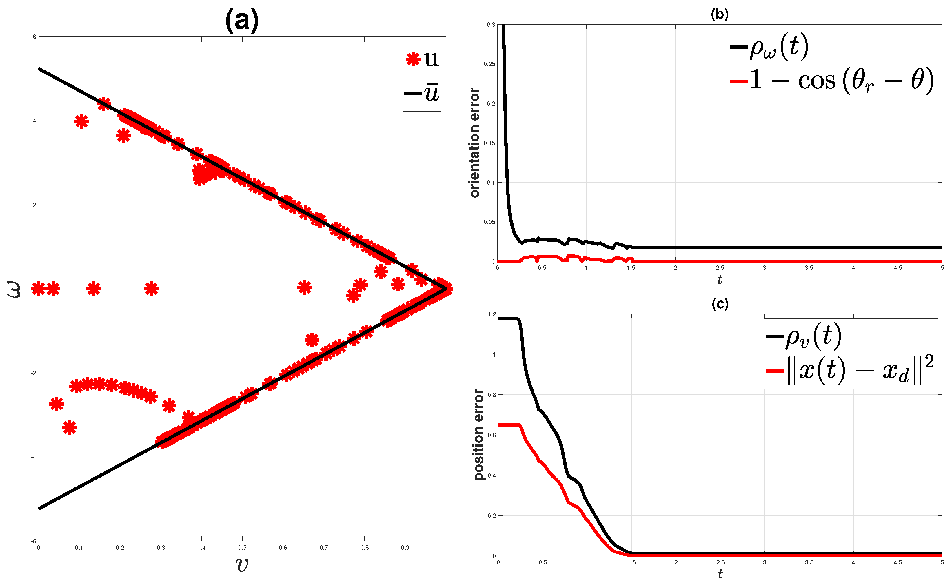
4.1. Motion Controller

The initial step of the proposed approach involves designing a control scheme to establish a well-defined transition according to Definition 6 to address the input constraints of the robot. Let p ( t k ) = [ x ( t k ) , y ( t k ) ] T F , specifically, p ( t k ) π k ( p ( t k ) π W ) for some t k R 0 and k K . Given δ R > 0 , the aim is to design a time-varying state-feedback control law u : F × [ t k , t ] U , with  t t k + δ , ensuring π k δ π ( π W δ π ). To achieve this, the free space is redefined as
F : =   W i J O i m M π m .
Henceforth, we aim to design a robust adaptive control scheme that addresses input limitations and guarantees the navigation among any two regions of interest in a prescribed time interval δ . We note that in cases of excessive input saturation, navigation in any arbitrarily prescribed time interval δ is not always possible. In such cases, the controller should ensure navigation between any two specified regions of interest in a time interval δ as close to the initially prescription as the limitations allow. The key to its functionality lies in transforming the free space F into a topologically equivalent yet geometrically simpler space. To achieve this, a diffeomorphism T : F P is employed, where P is a point world [37], i.e., an open disk modulo a finite set with cardinality equal to the number of obstacles and regions of interest | J | + | M | . The transformation described is not analytically derived but rather obtained through the solution of two boundary value problems, as described in [38] (pp. 14–17). The feedback controller that we propose ensures the prescribed navigation by adeptly avoiding obstacles. It guarantees that the distance p ( t ) c remains less than ρ v ( t ) , where ρ v ( t ) is an adaptive performance function that will be designed later. Let us now provide a path planner, which was initially proposed in [30], designed to ensure the secure navigation of holonomic mobile robots within spherical environments that are densely populated with static obstacles. The reference command is determined by the following law:
u r ( t , q ) = u γ ( t , q ) + u β ( q )
with u γ ( t , q ) = w ( t , q ) ( q q d ) , where q and q d represent the current position of the robot and its destination in the spherical world, respectively. The term w ( t , q ) corresponds to a state-dependent, time-varying control gain that vanishes as the robot approaches its destination point. The term u β ( q ) R 2 is activated when the robot approaches an obstacle beyond a predefined threshold, ensuring collision avoidance (additional details regarding (5) can be found in [30]). Note that the first term in (5) drives the robot towards its designated destination, while the second term is dedicated to enforcing collision avoidance, thus ensuring the forward invariance of the workspace. Henceforth, the control design is structured in three distinct steps, as outlined below.
Step 1. We define the normalized position error ξ v : =   p ( t ) c 2 ρ v ( t ) . Employing the coordinate transformation T : F P , we design the reference signal:
a ( t , p ) = J 1 ( T ( p ) ) k 1 ln 1 1 ξ v ( t ) ( 1 ξ v ( t ) ) ρ v ( t ) T ( p ) T ( p d ) + u β ( T ( p ) ) , k 1 > 0
where J ( · ) denotes the Jacobian of the coordinate mapping T ( · ) , and u β ( · ) is the collision avoidance term, as defined in [30]. When the motion of the robot is aligned with a ( t , p ) , i.e.,  p ˙ = a , then the prescribed time navigation problem regulated by the time parameter δ is solved for appropriately chosen parameters (see Theorem 1 in [30]). However, the pfaffian constraints, i.e., unicycle model of the robot, prevent the direct implementation of the reference signal a R 2 to the system (3), which leads us to the next design step.
Step 2. Given the reference vector a = [ a x , a y ] T R 2 , we define v r : =   a ( t , p ) and θ r : =   arctan a y a x , denoting its magnitude and direction, respectively. To avoid discontinuities of arctan ( · ) , we exploit the formula cos : =   ( θ r θ ) a x ( t , p ) a ( t , p ) cos ( θ ( t ) ) + a y ( t , p ) a ( t , p ) sin ( θ ( t ) ) to define the orientation error e ω : =   1 cos ( θ r θ ) [ 0 , 2 ] and the corresponding normalized error ξ ω : =   e ω ( t ) ρ ω ( t ) , with  ρ ω ( t ) denoting a performance function to be designed. Note that by imposing adaptive performance attributes to the normalized orientation error ξ ω , we ensure that e ω ( t ) < ρ ω ( t ) , t 0 . Since aligning with the direction of a ( t , p ) is crucial for ensuring collision avoidance, the fulfillment of orientation error constraints takes precedence over that of position constraints. To quantify this priority, we define the reference translational velocity as
v d ( t , p ) = s μ ( ρ ω ( t ) ) v r ( t , p )
with the following smooth bump function:
s μ ( ρ ω ( t ) ) = 0 if ρ ω ( t ) > μ ρ ω 2 ρ ω ( t ) ρ ω ρ ω ( μ 1 ) 3 3 ρ ω ( t ) ρ ω ρ ω ( μ 1 ) 2 + 1 if ρ ω ρ ω ( t ) μ ρ ω
with μ N { 1 } , and ρ ω denotes a performance parameter that will be defined later along with ρ ω ( t ) . In this manner, the reference translational velocity v d ( t , p ) is set to zero, i.e., the robot is commanded to stop, when the orientation error exceeds a safety threshold μ ρ ω . This pause continues until the robot aligns its orientation with the direction of (6), thereby ensuring secure navigation within the workspace. Note that when ρ ω ( t ) = ρ ω , then s μ ( ρ ω ) = 1 , which implies that v d = v r . Moreover, we design the reference angular velocity as follows:
ω d ( t , p ) = k 2 sign ( sin ( θ r θ ) ) ln 1 1 ξ ω ( t ) ( 1 ξ ω ( t ) ) ρ ω ( t ) , k 2 > 0 .
Step 3. In step 2, we designed the reference control input u d : =   [ v d ( t ) , ω d ( t ) ] T R 2 that ensures safe navigation with performance guarantees. Nevertheless, since u d ( t ) is constrained within the compact set U , we leverage a saturation function to produce the actual control input that obeys the input constraints. Hence, by selecting v ¯ = a and ω ¯ = a / b as the translational and rotational velocity saturation levels, respectively, we design a saturation function σ ( · ) : ( , ) × ( , ) U that maps the desired control signals u d U onto the boundary of the set U based on the radial distance of u d from the origin. The diamond-shaped input constraints illustrating the functionality of saturation function σ ( · ) are depicted in Figure 1. Thus, the control input incorporating both input and output constraints is obtained as follows:
u : =   [ u v ( t , p ) , u ω ( t , p ) ] T = σ ( u d ( t ) ) U .
Finally, in order to provide the necessary compromise between input and output constraints, we build on the Adaptive Performance Control (APC) technique [31], to introduce the following adaptive performance laws:
ρ ˙ v = s μ ( ρ ω ( t ) ) λ 1 ( ρ v ( t ) ρ v ) + | u v ( t , p ) v d ( t , p ) | , λ 1 , ρ v > 0
ρ ˙ ω = λ 2 ( ρ ω ( t ) ρ ω ) + | u ω ( t , p ) ω d ( t , p ) | , λ 2 , ρ ω > 0 .
with ρ v ( 0 ) > p ( 0 ) c 2 and ρ ω ( 0 ) > e ω ( 0 ) . Note that the performance specifications are incorporated through the parameters λ i , i = 1 , 2 , i.e., the convergence rate, and  ρ i , i { v , ω } , i.e., the maximum allowable steady-state error when saturation is inactive.
Remark 1. 
The performance parameters in (10) define the specifications regarding the position error p ( t ) c 2 , indicating both the maximum duration and the accuracy with which the robot will approach the desired position c . By choosing λ 1 > 1 δ ln η 2 ρ 1 ρ 1 ( 0 ) ρ 1 and ρ 1 < η 2 , the proposed control scheme (6)–(11) ensures that the robot will either reach c within a radius of η in a time interval less than δ or, in the case that transition within the time interval δ cannot be achieved, ensure the best feasible navigation time while obeying the input constraints. Concerning the performance parameters in (11), it is preferable to choose a value of λ 2 that is relatively large and a value of ρ 2 that is relatively small. This selection enables the rapid and accurate tracking of the direction of the reference vector (6), which is crucial for collision avoidance.
Remark 2. 
Note that the first term in both (10) and (11) is negative, enforcing the output constraints on the respective errors. Conversely, the second term is non-negative and becomes active when the corresponding control input reaches saturation. This activation ensures the necessary trade-off between input and output constraints. It is worth highlighting that when saturation is inactive, the adaptive performance functions revert to their prescribed form with the exponential rate dictated by the parameters λ i , i = 1 , 2 .
In order to clarify the functionality of the proposed controller, we present a simple illustrative paradigm. In this simulation, a mobile robot is commanded to navigate safely to a predetermined position inside a workspace within a specified time period of δ = 5 s or less. Figure 2 depicts both the real workspace (left) and the transformed sphere world (right). In these figures, the initial position of the robot is denoted by a green triangle, while the destination is denoted by a red ’x’. One can see that the proposed controller safely navigates the robot within the workspace and appropriately steers it to avoid collisions with the static obstacles (denoted by blue and purple boxes). The constrained control input u = [ u v , u ω ] T and the diamond-shaped input constraints are depicted in Figure 3a. Evidently, the control input obeys the input constraints, i.e.,  u ( t ) U for all t 0 . The orientation and position errors are depicted in Figure 3b,c, respectively. Notice that at the beginning of the simulation, the robot remains static until the performance function incorporating the orientation error specifications drops below a prespecified threshold, i.e., until s μ ( ρ ω ( t ) ) > 0 . Furthermore, the predefined temporal constraint, i.e.,  δ = 5  s, is achieved despite the presence of input saturation, as the decaying rate λ 1 , which determines the navigation time, has been set large enough to provide convergence to the destination at approximately t = 1.5  s.
The main properties of the proposed control strategy are outlined in the following theorem.
Theorem 1. 
Consider a unicycle robot described by (3) operating within a planar environment cluttered with obstacles and subject to the input constraints outlined in Section 3. The proposed control scheme (6)–(11) ensures the safe navigation of the robot within the workspace, preventing collisions and guiding the robot to its desired destination while also ensuring the following:
p ( t ) c 2 < ρ v ( t ) 1 cos ( θ r θ ) < ρ ω ( t ) , t 0 .
Proof. 
Let us first define the transformed errors ϵ v ln ( 1 1 ξ v ( t ) ) and ϵ ω ln ( 1 1 ξ ω ( t ) ) . Subsequently, consider the positive definite function V = 1 2 ϵ v 2 + ϵ ω 2 . Differentiating with respect to time, we get
V ˙ = ϵ v ( t ) ( 1 ξ v ( t ) ) ρ v ( t ) 2 ( p c ) T p ˙ ρ ˙ v ξ v + ϵ ω ( t ) ( 1 ξ ω ( t ) ) ρ ω ( t ) sin ( θ r ( t ) θ ( t ) ) θ ˙ r ω ρ ˙ ω ξ ω .
Substituting the control protocol (6)–(11) into V ˙ , we obtain
V ˙ = ϵ v ( t ) ( 1 ξ v ( t ) ) h 1 ( t , p , ρ v , ρ ω ) ζ 1 ( ϵ v ) + ϵ ω ( t ) ( 1 ξ ω ( t ) ) h 2 ( t , p , θ , θ r , θ ˙ r , ρ ω ) ζ 2 ( ϵ ω )
with
h 1 ( t , p , ρ v , ρ ω ) = 1 ρ v ( t ) ( p c ) T p ˙ + p ( t ) c 2 s μ ( ρ ω ( t ) ) λ 1 1 ρ v ρ v ( t ) h 2 ( t , p , θ , θ r , θ ˙ r , ρ ω ) = 1 ρ ω ( t ) sin ( θ r ( t ) θ ( t ) ) θ ˙ r ω + e ω ( t ) λ 2 1 ρ ω ρ ω ( t ) ζ 1 ( ϵ v ) = ξ v | u v ( t ) v d ( t ) | ζ 2 ( ϵ ω ) = ξ ω | u ω ( t ) ω d ( t ) | .
Owing to the continuity of s μ ( ρ ω ( t ) ) , θ r ( t ) , θ ˙ r , the fact that the system (3) is input-to-state stable, and the boundedness of the control input u ( t ) because of input constraints, it is concluded that there exist H 1 , H 2 > 0 such that h 1 ( · ) H 1 and h 2 ( · ) H 2 . These bounds are independent of upper bounds on ρ v ( t ) , ρ ω . Moreover, notice that 1 ( 1 ξ v ( t ) ) , 1 ( 1 ξ ω ( t ) ) > 1 , since | ξ v ( t ) | , | ξ ω | < 1 . Additionally, the continuous functions ζ 1 ( ϵ v ) , ζ 2 ( ϵ ω ) are strictly increasing and radially unbounded, and the transformed errors satisfy ϵ v ( t ) , ϵ ω ( t ) 0 , which leads to
V ˙ H 1 ζ 1 ( ϵ v ) ϵ v ( t ) + H 2 ζ 2 ( ϵ ω ) ϵ ω ( t ) .
Consequently, V ˙ becomes negative when ϵ v ( t ) > ζ 1 1 ( H 1 ) and ϵ ω ( t ) > ζ 2 1 ( H 2 ) . Furthermore, since ϵ v ( 0 ) and ϵ ω ( 0 ) are well defined, it can be concluded that ϵ v ( t ) , ϵ ω ( t ) are uniformly ultimately bounded, which implies that ξ v ( t ) , ξ ω ( t ) < 1 for all t 0 . Hence, it is deduced that all closed-loop signals remain bounded, as well as that p ( t ) c 2 < ρ v ( t ) and e ω < ρ ω ( t ) , t 0 , completing the proof.    □

4.2. High-Level Plan Generation

The next step in our solution involves devising a high-level timed plan spanning the regions of interest to satisfy the specified timed formula ϕ . This part is similar to the respective part in [10], and we provide a concise summary here. Leveraging the control mechanism introduced earlier, which enables transitions within the set Π , we first abstract the robot’s motion into a finite transition system denoted as T : = ( Π ˜ , Π ˜ 0 , , A P , L ˜ , γ ) , where γ : ( ) R > 0 assigns a cost to each transition, representing the distance that the robot needs to travel. This cost is intricately linked to the number and positions of obstacles and cannot be directly calculated. In the learning algorithm detailed in Section 4.3, we initially set γ ( π k π ) = | c k c | , γ ( π k π k ) = 0 , and γ ( π W π k ) = γ ( π k π W ) = | c k x ( 0 ) | , for all k , , K with k . These values are updated as the robot navigates through the workspace. Subsequently, the timed formula ϕ over the atomic propositions AP is translated to the TBA A t = ( Q , Q 0 , C L , AP , E , F ) using off-the-shelf tools [39]. Following that, we calculate the product Büchi Automaton A P as A P : =   T A t = ( S , S 0 , P , F P , γ P )  [10]. Starting from S 0 , we employ graph-search techniques to find the optimal path to the accepting states F P with respect to the cost γ P , which satisfies ϕ [7,40]. Using the abbreviation s I s for ( s , g , R , s ) in the set of edges of A P , such a path has the following form:
s ¯ p 0 I 0 , 1 s ¯ p 1 I 1 , 2 I L 1 , L s ¯ p L I L , L + 1 I L , L + 1 ( s ¯ p L + 1 I L + 1 , L + 2 I L + Z 1 , L + Z s ¯ p L + Z ) f
The first part of the path contains a finite prefix, meaning a finite sequence of states to be visited. The second part of the path, contained in the parentheses, is an infinite suffix, which is a specific sequence of states to be visited infinitely many times. This infinite frequency of visitation is represented by f. Additionally, s ¯ p j , j { 0 , , L + Z } , denotes the sequence
s ¯ p j : =   ( π p j , q j 0 ) I j 0 , 1 I j ( j 1 ) , j ( π p j , q j j )
with π p j Π ˜ , q j ι Q for j { 0 , , L + Z } , ι { 1 , , l j } and j { 0 , , | S | } . Moreover, q ( j + 1 ) 0 = q j j , q ( L + Z ) ( L + Z ) = q ( L + 1 ) 0 , and
I j , j + 1 : =   { q j , j + 1 , R j , j + 1 } , I j ι , ι + 1 : =   { q j ι , ι + 1 , R j ι , ι + 1 }
indicate the corresponding guards and reset maps for  j { 0 , 1 , , L + Z 1 } , ι { 0 , , j 1 } . The transition set I L + Z , L + 1 is defined similarly. Consider now the transitions
( π p j , q j 0 ) I j 0 , 1 I j ( j 1 ) , j ( π p j , q j j ) ( I j , j + 1 ) ( π p ( j + 1 ) , q ( j + 1 ) 0 )
that encode the physical transition from π p j to π p j + 1 in A P . The overlap between the respective guards g j , j + 1 and g ι , ι + 1 , where ι 0 , , j 1 , defines a time interval I j , j + 1 [ a , b ] , [ a , b ) , ( a , b ] , ( a , b ) , [ a , ) , ( a , ) with a , b Q > 0 and b > a . This interval satisfies t j , j + 1 I j , j + 1 if t j , j + 1 satisfies g j , j + 1 and g ι , ι + 1 for ι 0 , , j 1 , where t j , j + 1 represents the duration of the navigation from π j to π j + 1 . Similarly to [10], we frame the assignment of these transition times as a convex optimization problem. To do this, let t p : =   [ t 0 , 1 , , t L + Z 1 , L + Z , t L + Z , L + 1 ] R > 0 L + Z + 1 be the concatenation of the transition times, and let L b : =   [ l b 0 , 1 , , l b L + Z 1 , L + Z , l b L + Z , L + 1 ] represent the lower bounds for this variable. The optimization problem is as follows:
min t p j = 0 L + Z 1 ( γ ( π p j π p j + 1 ) t j , j + 1 ) + γ ( π p L + Z π p L + 1 ) t j , j + 1
s . t . t j , j + 1 I j , j + 1 , t L + Z , L + 1 I L + Z , L + 1 t j , j + 1 l b j , j + 1 , t L + Z , L + 1 l b L + Z , L + 1
for j { 0 , L + Z } . In addition to enforcing constraints arising from guard intersections, limitations are imposed on the inputs through L b . Failing to consider these bounds may result in the assignment of transition times that are unattainable due to input constraints. Similarly to the cost γ , these bounds are heavily influenced by the presence of obstacles among regions and the input constraints, making a priori computation unfeasible. In the learning algorithm outlined in Section 4.3, we initialize these bounds based on the initial costs and the input saturation level v ¯ : l b π k π l = | c k c | v ¯ , l b π k π k = 0 , and  l b π W π k = l b π k π W = | c k x ( 0 ) | v ¯ , for all k , , K with k . These values are updated as the robot navigates in the workspace. Furthermore, it is important to note that the objective function in (13) is a convex function of t p , and the constraints can be expressed as linear inequalities and lower bounds on the problem variables. Consequently, the optimization problem described above is convex and can be efficiently solved using off-the-shelf software. The choice of this specific cost function is motivated by two observations: (i) the time assigned to a transition is an increasing function of the transition cost, and (ii) shorter transition times are penalized.

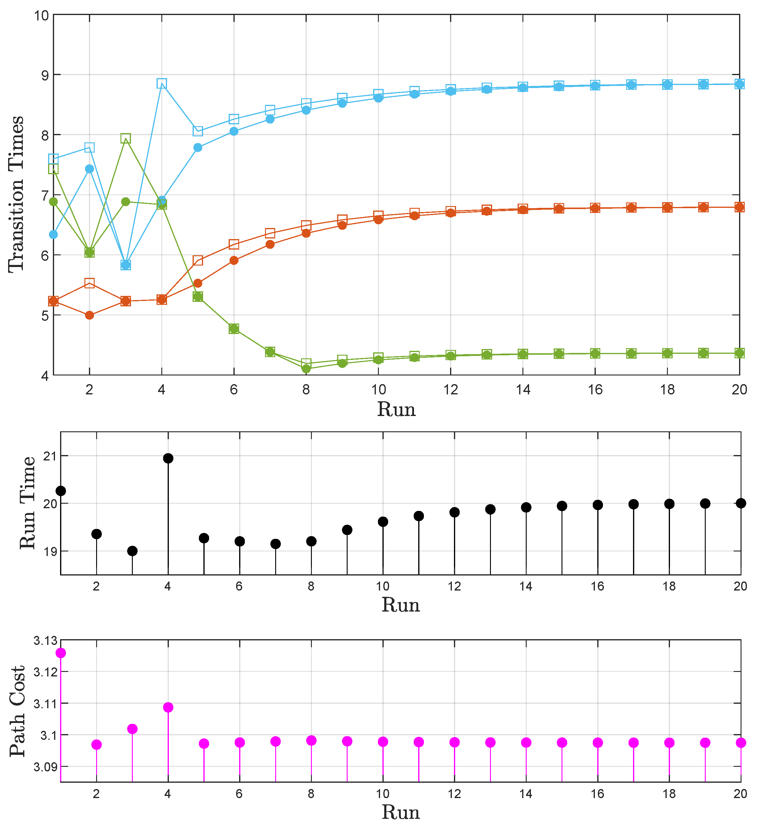
4.3. Iterative Learning

The third part of the solution is an iterative procedure that is depicted in Algorithm 1 and derives feasible paths and transition times. After the optimization problem (13) and (14) is solved and the time durations t p have been attained (line 8), the robot performs each transition using the motion controller presented in Section 4.1 (line 9). Once transition π p j ( t j , j + 1 ) π p j + 1 is completed, the corresponding transition cost γ ( π j π j + 1 ) is updated with the length of the curve for the duration of the transition (line 10), which is more accurate than the initial Euclidean-based estimate; the obstacles obstruct the straight-line path between two regions of interest. The lower time bound required to perform the transition l b π j π j + 1 is also updated accordingly. Specifically, this bound is updated only if the transition duration takes longer time than the time requested (line 11–14).
With this new information, the associated optimization problem is resolved to acquire new transition times (line 8). Notably, after each transition, the optimization problem constraints are altered. Particularly, the TBA of the formula is shifted forward by a time amount equal to the last performed transition, which induces a change in the guards and, therefore, in the constraints.
Algorithm 1 Iterative Learning Algorithm
Input: Product Büchi Automaton A P , Initial position π 0 , Formula ϕ , Input Constraint level v ¯
Output: Optimal Cost Path: P a t h
1:
Γ I n i t i a l i z e C o s t s ( π 0 )
2:
L b I n i t i a l i z e T i m e B o u n d s ( π 0 , C o s t s , v ¯ )
3:
P a t h
4:
while  P a t h ¬ ϕ do
5:
     P a t h i G r a p h S e a r c h ( A P , π 0 , Γ )
6:
    for  j 1 to ( L e n g t h ( P a t h i ) 1 )  do
7:
         π p j P a t h i ( j ) , π p j + 1 P a t h i ( j + 1 )
8:
         t j , j + 1 S o l v e ( ( , ) , Γ , L b )
9:
         P e r f o r m ( π p j π p j + 1 )
10:
         U p d a t e C o s t s ( Γ , γ ( π p j , π p j + 1 ) )
11:
        if ( π p j π p j + 1 ) not achieved in t j , j + 1  then
12:
            l b j , j + 1 t j , j + 1 ( a c t u a l )
13:
            U p d a t e B o u n d s ( L b , l b j , j + 1 )
14:
        else  t j , j + 1 ( a c t u a l ) t j , j + 1
15:
     U p d a t e P a t h ( P a t h , γ ( π p j , π p j + 1 ) , t j , j + 1 ( a c t u a l ) )
16:
return  P a t h
After each path is run, the algorithm repositions the robot in the initial state x ( 0 ) using the motion controller (Section 4.1) to explore new potential paths. This repositioning allows for an exhaustive search of timed paths, eventually deriving the one that optimally satisfies the task with respect to the traveled distance. We stress that the learning algorithm of our previous work [10], which did not accommodate input constraints, considered a fixed path by only updating the time constraints of the optimization (13) and (14). Such a setting is conservative, since the timed task might not be satisfied by all possible paths due to the input constraints, regardless of the assigned times.
Remark 3. 
Regarding the time complexities of the framework, we note that the construction of the Product Automaton is an offline procedure that does not affect the online solution time-wise. Additionally, even though the optimization problem (13) and (14) has low computational complexity, computational overhead can also be accounted for by allocating the required time or by optimizing en route to the next region of interest. What does add to the time complexity, however, is the size of the graph representing the Product Automaton. This is linked to the intricacy of the specified timed formula ϕ and can prolong the graph-search stage and, therefore, the path selection stage. We note that the time complexity of the iterative algorithm aligns with the time complexity of the graph-search method employed. When selecting this method, one must take into account the size of the graph in order to ensure the completeness and optimality of the produced solution of the search.

5. Simulation Study

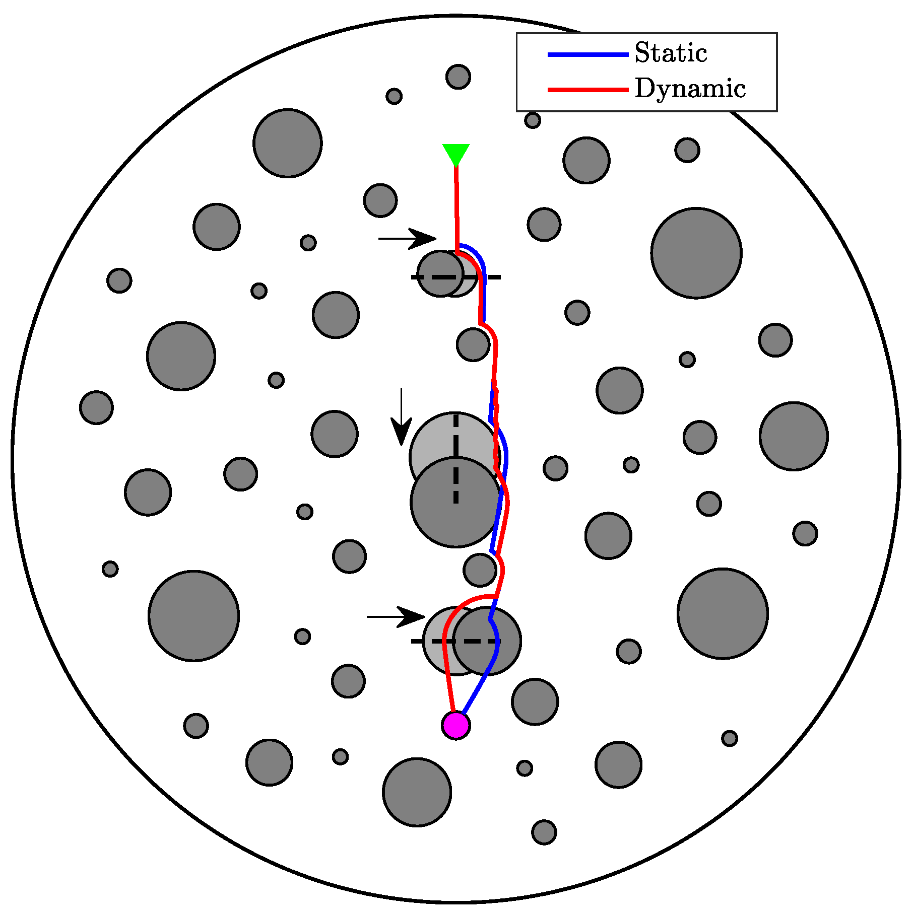
5.1. Dynamic Obstacle Environment

The first step of our simulation study involves showcasing the effectiveness of the proposed motion controller in workspaces occupied by dynamic obstacles. More specifically, we consider a sphere world (Figure 4) containing static obstacles along with three moving ones, which follow oscillatory trajectories denoted by dotted lines. Arrows represent suggestive directions of movement along each trajectory, and the dynamic obstacles are depicted at indicative time instances. From a starting configuration in the workspace (green triangle), we request a transition time of 10 time units (tu) for navigation to a destination region (purple circle). We repeat the same scenario in a static equivalent of the workspace by replacing the three moving obstacles with stationary ones, as displayed with the light gray color in Figure 4. Observing the two cases, it is evident that the controller ensures safe navigation in both static (blue path) and dynamic obstacle environments (red path). Furthermore, the scheme naturally attempts to achieve the requested transition time specifications, but the obstacle movement can add to the existing effect of the input constraints, increasing both the required distance and the necessary transition time, as shown in Table 1.

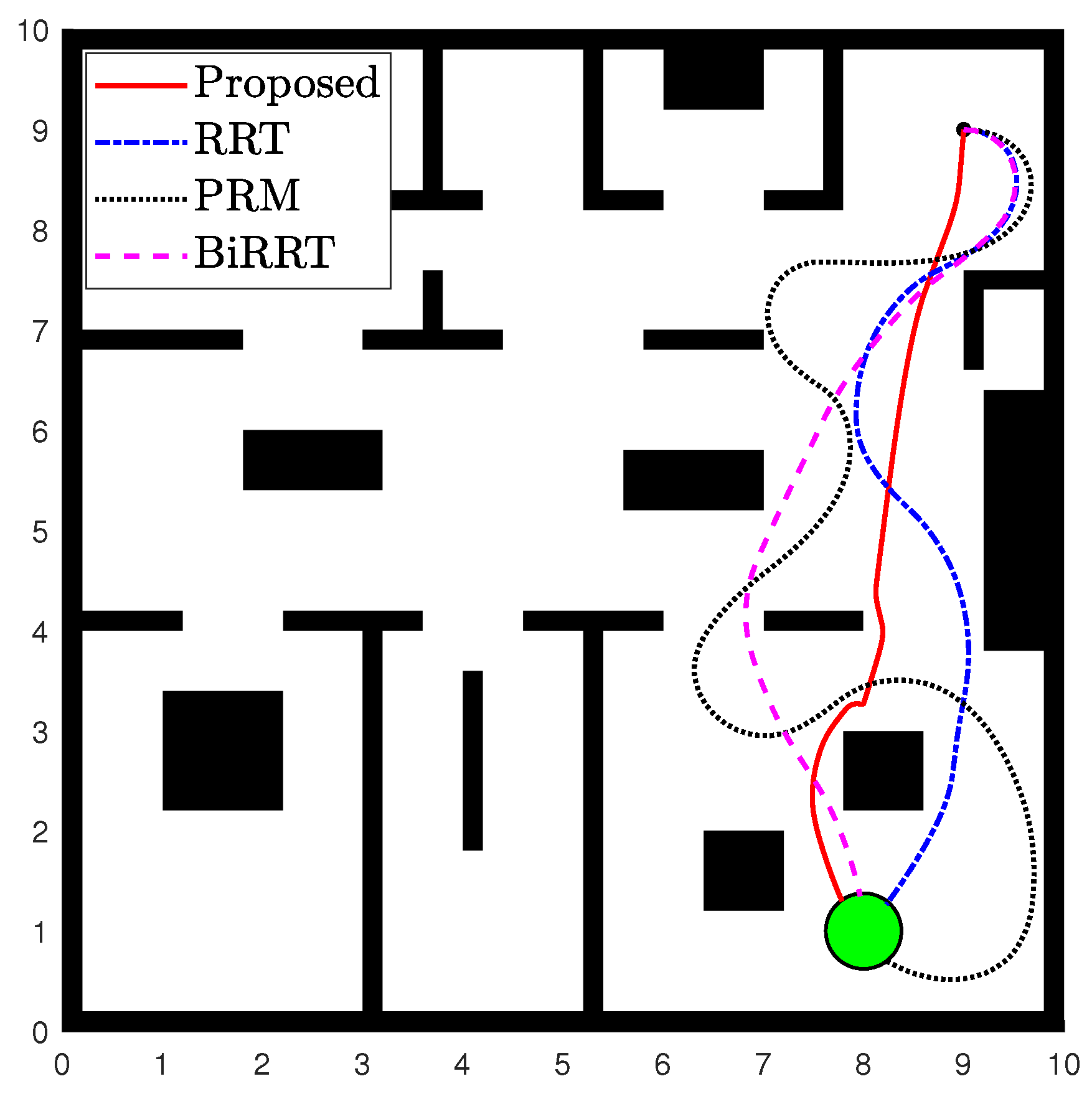
5.2. Comparison of Path Planners

In the following, we employ different planners to calculate the path between a starting configuration and a destination region in the workspace, and we subsequently assess their performance. To be precise, we utilize the following path planners:
  • Proposed motion controller (Section 4.1)
  • Rapidly Exploring Random Tree (RRT) planner
  • Probabilistic Road Map (PRM) planner
  • Bidirectional Rapidly Exploring Random Tree (BiRRT) planner
In addition, we examine the required transition time and the distance covered, since these metrics are essential for the effective application of the three-layer approach (Section 4). The scenario is illustrated in Figure 5. Examining the results in Table 2, it is evident that the proposed controller is more efficient in calculating the distance-wise optimal path. Additionally, it is the only one out of the four planners that can incorporate transition time requirements, which are necessary when tackling complex motion planning tasks. Finally, contrary to the other planners, the proposed scheme works online, rendering it more dexterous in dealing with complex and dynamic environments.

5.3. Examination of the Proposed Scheme

The complete proposed scheme is now exemplified through an extensive study. We consider an agent governed by the unicycle dynamics of Section 3, operating in an obstacle-cluttered environment with three regions of interest π k = B ¯ ( c k , r ) , which define the set Π = { π k } , k K . The set of atomic propositions is AP = Π ˜ , and the labeling function L ˜ : Π 2 AP is defined as π k { π k } , k K . Starting from an initial position in the free space F , we require the robot to “always visit each region of interest at least once every x time units”, corresponding to the following MITL formula:
ϕ = k K ( I π k ) , I = [ 0 , x ]
We examine the scheme in both a sphere and a generalized world. For each world, we additionally consider the following two cases:
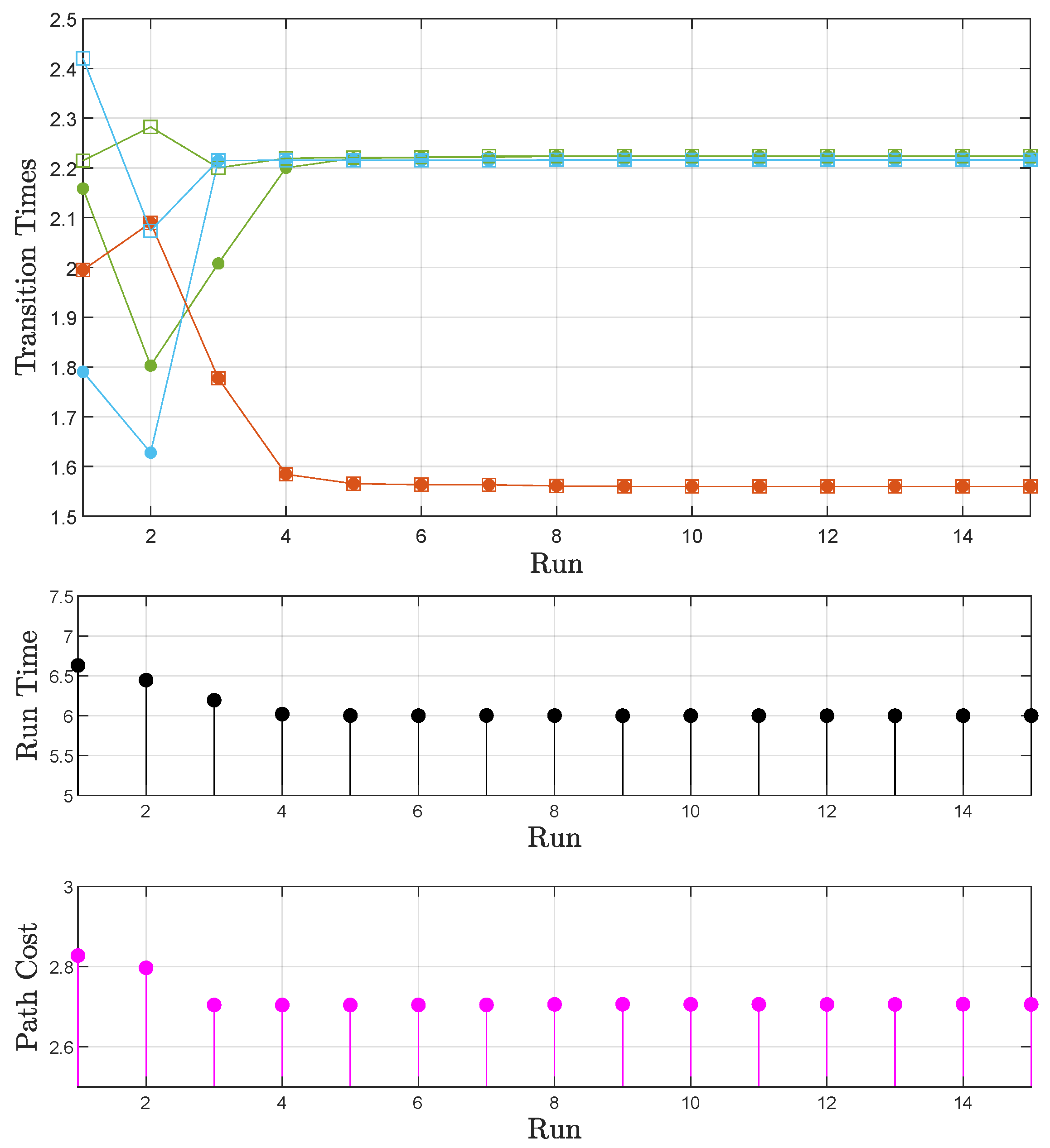
  • Case A: The time available for task execution is sufficient. After the reassignment of the transition times through the iterative learning algorithm, the satisfaction of the formula ϕ in the time frame I = [ 0 , x ] is possible.
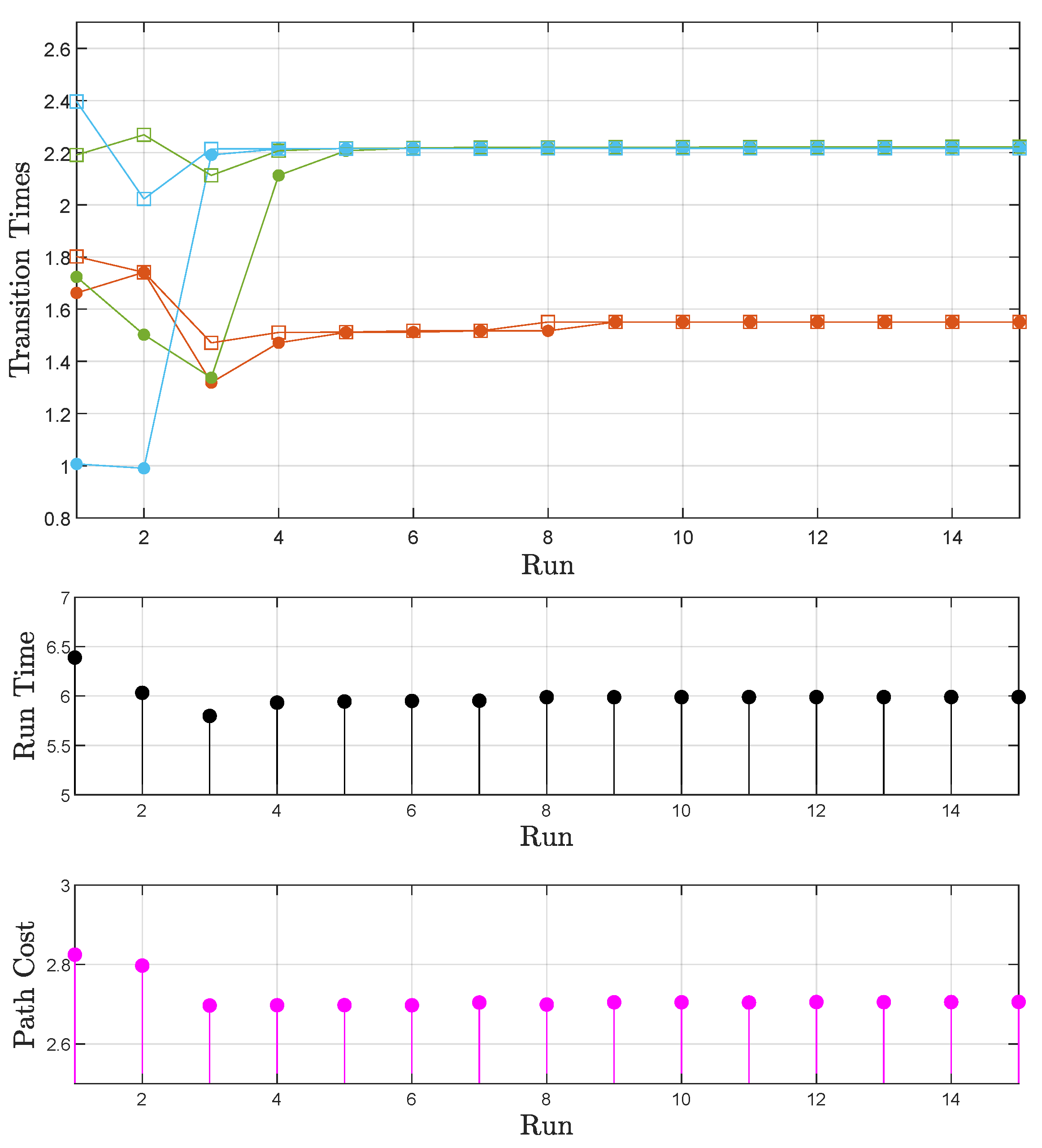
  • Case B: The time available for task execution is not sufficient. Here, the scheme should again be able to find the optimal path while also taking into account the inability to satisfy the formula ϕ in the requested time frame.

5.3.1. Sphere World

The agent operates in an obstacle-cuttered sphere world, as illustrated in Figure 6. The three regions of interest are denoted as discs (red, green, blue), and the initial position of the agent is the black dot.

Sphere World: Case A

We request a time frame of 20 time units ( I = [ 0 , 20 ] ) for the satisfaction of the formula ϕ . Using the Euclidean distances as the only initial knowledge regarding the different path options, the algorithm explores different routes, some with large costs and large runtimes (e.g., Run 1 Figure 7) and others with smaller distances but with heavier input saturation encountered and, therefore, larger runtimes (e.g., Run 4 Figure 7). The results are depicted in Figure 7. We observe that as the iterative learning process evolves, the transition times calculated by (13) and (14) converge to the actually used times (Figure 7 (top)). Moreover, the total runtime of the path (consisting of three individual transitions), while initially not satisfying the task (>20 tu), converges to a task-satisfying duration (Figure 7 (middle)). Finally, the path cost per suffix execution is reduced as the agent gathers information about the transition times and costs (Figure 7 (bottom)). The optimal path traced by the algorithm can be observed in Figure 6 (bottom).

Sphere World: Case B

For a requested time frame of 19 time units, the satisfaction of the formula is not possible. However, with convergence to a minimum cost with respect to the traveled distance, a path can still be achieved, as presented in Figure 8 (bottom). Additionally, we observe convergence to the actual time frame in which the task can be satisfied while simultaneously following the optimal-cost path (Figure 8 (middle)), which is again the one in Figure 6 (bottom). This time frame is obviously greater than the one initially requested (20 tu). This comes as a result of the progressively improved transition time assignment, which establishes the times corresponding to consistent transitions (Figure 8 (top)).

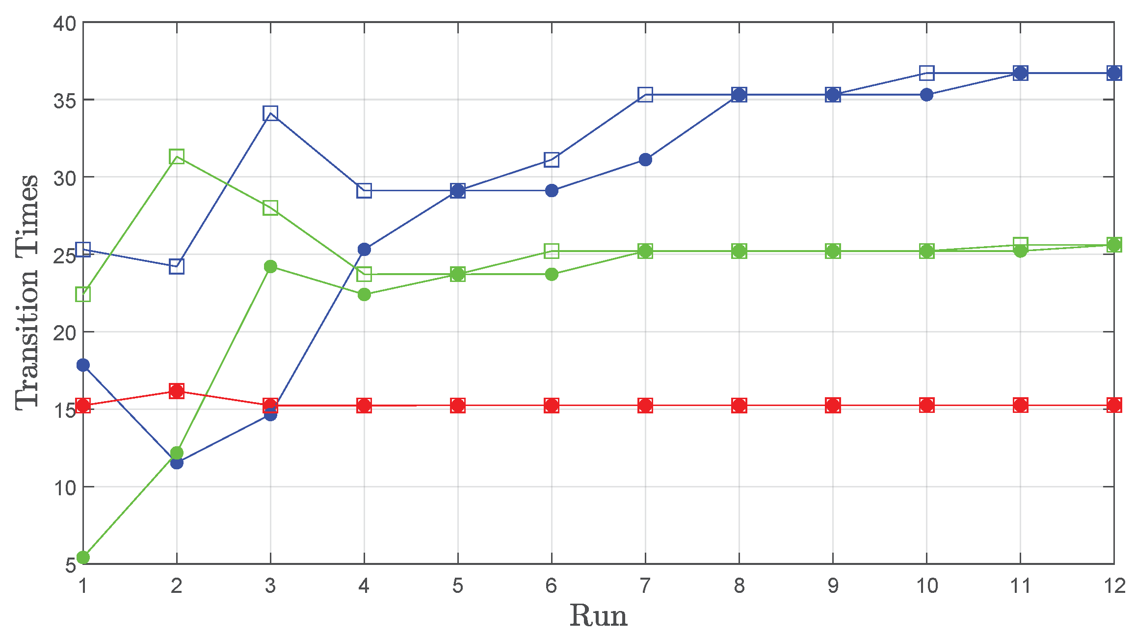
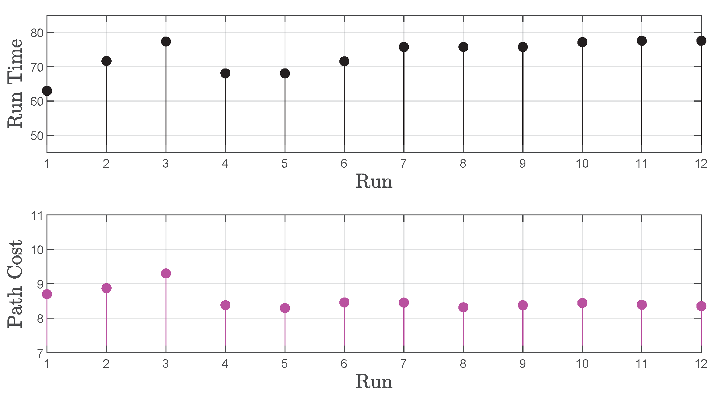
5.3.2. Generalized World

An agent operates in an office environment with three regions of interest. The scenario is illustrated in Figure 9. The regions of interest and the initial position remain the blue, green, and red discs and the black dot, respectively.

Generalized World: Case A

We seek a time frame of six time units ( I = [ 0 , 6 ] ) for the fulfillment of ϕ . The outcomes are illustrated in Figure 10. Similarly to the sphere world, as the iterative learning process advances, the transition times converge to the actual times (Figure 10 (top)). Additionally, although the total path runtime initially falls short of meeting the task requirement (>6 tu), it gradually converges to a duration that satisfies the task (Figure 10 (middle)). Lastly, the path cost decreases as the agent acquires information about the transition times and distances (Figure 10 (bottom). The optimal path found is the one depicted in Figure 9 (bottom).

Generalized World: Case B

While a requested time frame of five time units ( I = [ 0 , 5 ] ) does not allow satisfaction of the formula, convergence to a minimum-cost path (Figure 9 (bottom)) is still attainable, as illustrated in Figure 11 (bottom). Furthermore, there is observable convergence to the actual time frame necessary for task satisfaction while adhering to the optimal cost path (Figure 11 (middle)). The actual time frame surpasses the initially requested one of 5 tu (6 tu), a result of the progressively refined assignment of transition times, aligning them with consistent transitions (Figure 11 (top)).
In the context of both the sphere and generalized world cases, there are notable observations to consider. Firstly, as the accuracy of transition time assignment gradually improves, the optimal cost path may settle at a value slightly exceeding the initially calculated one during its primary traversal (see, for example, Figure 7 (bottom)). This outcome is attributed to the refined time assignment, preventing the agent from adopting a rushed approach and leading to transitions that are slightly smoother and more prolonged. Naturally, should the refined path cost value cease to represent the optimal path option, the algorithm would opt for an alternative, following a similar procedure.
Moreover, beyond the consideration of the path cost, it is evident that certain traversed paths (such as Run 3 in Figure 8) may appear achievable within the requested time frame. However, it is crucial to recognize that these paths may not be temporally reliable yet. To elaborate, they might involve transitions accomplished without the requested transition times accurately aligning with the actual durations (see, for example, Run 3 of the green transition in Figure 8). In practical terms, this implies that to achieve such a transition, a smaller time must be requested than what is actually needed. To purposely adopt such a practice, however, would mean forcing the agent to work through heavier saturation. Additionally, we would not acquire durations that result in consistent and time-wise repeatable transitions, which would be necessary for the completion of timed tasks. In the proposed algorithm, even though it may extend the given time frame post-convergence, assurance is established that the times assigned to each transition are not only consistent but also safe and repeatable, deeming the path temporally reliable.

6. Experimental Study

We also conducted an experimental study to verify the validity of our findings. We consider an AmigoBot mobile robot operating in a workspace with three regions of interest (blue, red, and yellow), as shown in Figure 12. An Odroid computer was attached to the AmigoBot to run the Robotic Operating System (ROS). Additionally, an RPLIDAR-A1 was mounted on the agent in order to extract the workspace map using Simultaneous Localization and Mapping (SLAM). More precisely, the map of the workspace was created using the gmapping ROS implementation [41,42], and the boundaries necessary for the diffeomorphism T : F P for scheme implementation in generalized worlds were extracted using OpenCV. Regarding the localization process, the ROS implementation deployed was Adaptive Monte Carlo Localization (AMCL) [43], utilizing odometry data and a laser scan to estimate the precise location of the agent in the workspace and provide online localization during each run. A basic schematic of the ROS setup can be observed in Figure 13.
Starting from an initial position in the free space, we require the robot to “always visit each region of interest at least once every 45 seconds”, corresponding to the MITL formula (15), with I = [ 0 , 45 ] s. The scenario is illustrated in Figure 12, indicative runs of the algorithm are depicted in Figure 14 and the results are shown in Figure 15. We can observe that the requested time frame is not sufficient for the satisfaction of the formula, but convergence to an optimal cost path is still achieved, as shown in Figure 15 (bottom). This path is depicted in Figure 14 (bottom). In Figure 15 (top), we examine the times corresponding to the three transitions of each path; red represents the first transition, green represents the second, and blue represents the third. The actual values of these individual transitions meet the ones calculated by the algorithm while simultaneously settling into the optimal-cost path. Finally, we detect convergence to the actual time frame in which the task can be satisfied in Figure 15 (middle). A video of the agent traversing a single indicative path and a video of the complete iterative learning process (12 Runs) can be accessed through the following hyperlinks:

7. Conclusions and Future Work

A novel three-layer algorithm designed to ensure timed temporal specifications within obstacle-cluttered environments in the presence of input constraints was proposed in this work. Through an iterative learning framework, a high-level plan adeptly generates navigation paths that adhere to specified timed requirements. The integration of a novel low-level controller that takes into account diamond input constraints ensures safe navigation within the workspace, optimizing navigation time while respecting input constraints. Validation through comparative simulations and real-world experimentation confirms the effectiveness and superiority of the proposed scheme. Future efforts will emphasize incorporating runtime considerations into optimal path selection criteria, exploring more intricate timed specifications and more complex workspaces and researching formula relaxation techniques. Future endeavors will prioritize integrating runtime considerations into optimal path selection criteria, exploring more intricate timed specifications, and investigating formula relaxation techniques. Additionally, extending the results to multi-agent systems subject to communication and safety constraints requires further investigation.

Author Contributions

Conceptualization, C.K.V. and C.P.B.; methodology, F.C.T. and P.S.T.; software, F.C.T. and T.-F.B.; validation, C.K.V. and C.P.B.; formal analysis, F.C.T. and P.S.T.; investigation, F.C.T. and P.S.T.; writing—original draft preparation, F.C.T. and P.S.T.; writing—review and editing, C.K.V. and C.P.B.; visualization, F.C.T.; supervision, C.K.V. and C.P.B.; project administration, C.P.B. All authors have read and agreed to the published version of the manuscript.

Funding

This work was funded by the Hellenic Foundation for Research and Innovation (H.F.R.I.) under the second call for research projects to support postdoctoral researchers (HFRI-PD19-370). The work of C.P.B. was also supported by the project “Applied Research for Autonomous Robotic Systems” (MIS 5200632), which is implemented within the framework of the National Recovery and Resilience Plan “Greece 2.0” (Measure: 16618- Basic and Applied Research) and is funded by the European Union—NextGenerationEU.

Institutional Review Board Statement

Not applicable.

Informed Consent Statement

Not applicable.

Data Availability Statement

The data presented in this study are available upon request from the corresponding author. The data are not publicly available due to privacy restrictions.

Conflicts of Interest

The authors declare no conflicts of interest.

Abbreviations

The following abbreviations are used in this manuscript:
MTLMetric Temporal Logic
MITLMetric Interval Temporal Logic
TBATimed Büchi Automaton
APCAdaptive Performance Control
R Set of real numbers
R 0 Set of non-negative numbers
R > 0 Set of positive numbers
· Absolute value of a scalar
· Spectral (euclidean) norm of a matrix (vector), respectively
· Infinity norm
ϕ MITL formula
F Free space
K Points of interest within the free space
L Labeling function
δ Prescribed time interval
θ Orientation of robot
uCommanded linear velocity of robot
ω Commanded angular velocity of robot
u d Nominal linear velocity of robot
ω d Nominal angular velocity of robot
ρ u , ρ ω Performance functions regarding the evolution of position and orientation error, respectively
s μ ( χ ) Continuous function vanishing when χ > μ χ min
σ ( χ ) Saturation function constraining the vector χ within a compact set based on the radial distance of χ from the origin

References

  1. Bhatia, A.; Kavraki, L.E.; Vardi, M.Y. Sampling-based motion planning with temporal goals. In Proceedings of the 2010 IEEE International Conference on Robotics and Automation, Anchorage, AK, USA, 3–7 May 2010; pp. 2689–2696. [Google Scholar]
  2. Belta, C.; Isler, V.; Pappas, G.J. Discrete abstractions for robot motion planning and control in polygonal environments. IEEE Trans. Robot. 2005, 21, 864–874. [Google Scholar] [CrossRef]
  3. Fainekos, G.E.; Girard, A.; Kress-Gazit, H.; Pappas, G.J. Temporal logic motion planning for dynamic robots. Automatica 2009, 45, 343–352. [Google Scholar] [CrossRef]
  4. Kloetzer, M.; Belta, C. Automatic deployment of distributed teams of robots from temporal logic motion specifications. IEEE Trans. Robot. 2009, 26, 48–61. [Google Scholar] [CrossRef]
  5. Kress-Gazit, H.; Fainekos, G.E.; Pappas, G.J. Temporal-logic-based reactive mission and motion planning. IEEE Trans. Robot. 2009, 25, 1370–1381. [Google Scholar] [CrossRef]
  6. Loizou, S.G.; Kyriakopoulos, K.J. Automatic synthesis of multi-agent motion tasks based on ltl specifications. In Proceedings of the 2004 43rd IEEE conference on decision and control (CDC)(IEEE Cat. No. 04CH37601), Nassau, Bahamas, 14–17 December 2004; Volume 1, pp. 153–158. [Google Scholar]
  7. Guo, M.; Johansson, K.H.; Dimarogonas, D.V. Motion and action planning under LTL specifications using navigation functions and action description language. In Proceedings of the 2013 IEEE/RSJ International Conference on Intelligent Robots and Systems, Tokyo, Japan, 3–7 November 2013; pp. 240–245. [Google Scholar]
  8. Bouyer, P.; Laroussinie, F.; Markey, N.; Ouaknine, J.; Worrell, J. Timed temporal logics. In Models, Algorithms, Logics and Tools: Essays Dedicated to Kim Guldstrand Larsen on the Occasion of His 60th Birthday; Springer: Cham, Switzerland, 2017; pp. 211–230. [Google Scholar]
  9. Verginis, C.K.; Dimarogonas, D.V. Timed abstractions for distributed cooperative manipulation. Auton. Robot. 2018, 42, 781–799. [Google Scholar] [CrossRef]
  10. Verginis, C.K.; Vrohidis, C.; Bechlioulis, C.P.; Kyriakopoulos, K.J.; Dimarogonas, D.V. Reconfigurable motion planning and control in obstacle cluttered environments under timed temporal tasks. In Proceedings of the 2019 International Conference on Robotics and Automation (ICRA), Montreal, QC, Canada, 20–24 May 2019; pp. 951–957. [Google Scholar]
  11. Faied, M.; Mostafa, A.; Girard, A. Dynamic optimal control of multiple depot vehicle routing problem with metric temporal logic. In Proceedings of the 2009 American Control Conference, St. Louis, MO, USA, 10–12 June 2009; pp. 3268–3273. [Google Scholar]
  12. Fu, J.; Topcu, U. Computational methods for stochastic control with metric interval temporal logic specifications. In Proceedings of the 2015 54th IEEE Conference on Decision and Control (CDC), Osaka, Japan, 15–18 December 2015; pp. 7440–7447. [Google Scholar]
  13. Karaman, S.; Frazzoli, E. Vehicle routing problem with metric temporal logic specifications. In Proceedings of the 2008 47th IEEE Conference on Decision and Control, Cancun, Mexico, 9–11 December 2008; pp. 3953–3958. [Google Scholar]
  14. Edelkamp, S.; Lahijanian, M.; Magazzeni, D.; Plaku, E. Integrating temporal reasoning and sampling-based motion planning for multigoal problems with dynamics and time windows. IEEE Robot. Autom. Lett. 2018, 3, 3473–3480. [Google Scholar] [CrossRef]
  15. Zhou, Y.; Maity, D.; Baras, J.S. Timed automata approach for motion planning using metric interval temporal logic. In Proceedings of the 2016 European Control Conference (ECC), Aalborg, Denmark, 29 June–1 July 2016; pp. 690–695. [Google Scholar]
  16. Andersson, S.; Nikou, A.; Dimarogonas, D.V. Control synthesis for multi-agent systems under metric interval temporal logic specifications. IFAC-PapersOnLine 2017, 50, 2397–2402. [Google Scholar] [CrossRef]
  17. Nikou, A.; Boskos, D.; Tumova, J.; Dimarogonas, D.V. On the timed temporal logic planning of coupled multi-agent systems. Automatica 2018, 97, 339–345. [Google Scholar] [CrossRef]
  18. Verginis, C.K.; Dimarogonas, D.V. Distributed cooperative manipulation under timed temporal specifications. In Proceedings of the 2017 American Control Conference (ACC), Seattle, WA, USA, 24–26 May 2017; pp. 1358–1363. [Google Scholar]
  19. Wang, W.; Schuppe, G.; Tumova, J. Decentralized Multi-agent Coordination under MITL Specifications and Communication Constraints. In Proceedings of the 2023 31st Mediterranean Conference on Control and Automation (MED), Limassol, Cyprus, 26–29 June 2023; pp. 842–849. [Google Scholar]
  20. Hustiu, S.; Dimarogonas, D.; Mahulea, C.; Kloetzer, M. Multi-robot Motion Planning under MITL Specifications based on Time Petri Nets. In Proceedings of the 2023 European Control Conference (ECC), Bucharest, Romania, 13–16 June 2023. [Google Scholar]
  21. Gol, E.A.; Belta, C. Time-constrained temporal logic control of multi-affine systems. Nonlinear Anal. Hybrid Syst. 2013, 10, 21–33. [Google Scholar] [CrossRef]
  22. He, K.; Lahijanian, M.; Kavraki, L.E.; Vardi, M.Y. Towards manipulation planning with temporal logic specifications. In Proceedings of the 2015 IEEE International Conference on Robotics and Automation (ICRA), Seattle, WA, USA, 26–30 May 2015; pp. 346–352. [Google Scholar]
  23. Barbosa, F.S.; Lindemann, L.; Dimarogonas, D.V.; Tumova, J. Integrated Motion Planning and Control Under Metric Interval Temporal Logic Specifications. In Proceedings of the 2019 18th European Control Conference (ECC), Naples, Italy, 25–28 June 2019; pp. 2042–2049. [Google Scholar]
  24. Seong, H.; Lee, K.; Cho, K. Reactive Planner Synthesis Under Temporal Logic Specifications. IEEE Access 2024, 12, 13260–13276. [Google Scholar] [CrossRef]
  25. Huang, Z.; Lan, W.; Yu, X. A Formal Control Framework of Autonomous Vehicle for Signal Temporal Logic Tasks and Obstacle Avoidance. IEEE Trans. Intell. Veh. 2024, 9, 1930–1940. [Google Scholar] [CrossRef]
  26. Yu, X.; Yin, X.; Lindemann, L. Efficient STL Control Synthesis Under Asynchronous Temporal Robustness Constraints. In Proceedings of the 2023 62nd IEEE Conference on Decision and Control (CDC), Singapore, 13–15 December 2023; pp. 6847–6854. [Google Scholar]
  27. Li, S.; Park, D.; Sung, Y.; Shah, J.; Roy, N. Reactive Task and Motion Planning under Temporal Logic Specifications. In Proceedings of the 2021 IEEE International Conference on Robotics and Automation (ICRA), Xi’an, China, 30 May–5 June 2021; pp. 9228–9234. [Google Scholar]
  28. Fotiadis, F.; Verginis, C.K.; Vamvoudakis, K.G.; Topcu, U. Assured learning-based optimal control subject to timed temporal logic constraints. In Proceedings of the 2021 60th IEEE Conference on Decision and Control (CDC), Austin, TX, USA, 14–17 December 2021; pp. 750–756. [Google Scholar]
  29. Bonnah, E.; Nguyen, L.; Hoque, K. Motion Planning Using Hyperproperties for Time Window Temporal Logic. IEEE Robot. Autom. Lett. 2023, 8, 4386–4393. [Google Scholar] [CrossRef]
  30. Vrohidis, C.; Vlantis, P.; Bechlioulis, C.P.; Kyriakopoulos, K.J. Prescribed time scale robot navigation. IEEE Robot. Autom. Lett. 2018, 3, 1191–1198. [Google Scholar] [CrossRef]
  31. Trakas, P.S.; Bechlioulis, C.P. Approximation-free Adaptive Prescribed Performance Control for Unknown SISO Nonlinear Systems with Input Saturation. In Proceedings of the 2022 IEEE 61st Conference on Decision and Control (CDC), Cancun, Mexico, 6–9 December 2022; pp. 4351–4356. [Google Scholar]
  32. Alur, R.; Dill, D.L. A theory of timed automata. Theor. Comput. Sci. 1994, 126, 183–235. [Google Scholar] [CrossRef]
  33. Bouyer, P.; Markey, N.; Ouaknine, J.; Worrell, J. The cost of punctuality. In Proceedings of the 22nd Annual IEEE Symposium on Logic in Computer Science (LICS 2007), Wroclaw, Poland, 10–14 July 2007; pp. 109–120. [Google Scholar]
  34. D’Souza, D.; Prabhakar, P. On the expressiveness of MTL in the pointwise and continuous semantics. Int. J. Softw. Tools Technol. Transf. 2007, 9, 1–4. [Google Scholar] [CrossRef]
  35. Ouaknine, J.; Worrell, J. On the decidability of metric temporal logic. In Proceedings of the 20th Annual IEEE Symposium on Logic in Computer Science (LICS’05), Chicago, IL, USA, 26–29 June 2005; IEEE: Piscataway, NJ, USA, 2005; pp. 188–197. [Google Scholar]
  36. Chen, X.; Jia, Y.; Matsuno, F. Tracking Control for Differential-Drive Mobile Robots With Diamond-Shaped Input Constraints. IEEE Trans. Control Syst. Technol. 2014, 22, 1999–2006. [Google Scholar] [CrossRef]
  37. Loizou, S.G. The navigation transformation. IEEE Trans. Robot. 2017, 33, 1516–1523. [Google Scholar] [CrossRef]
  38. Vlantis, P. Distributed Cooperation of Multiple Robots under Operational Constraints via Lean Communication. Ph.D. Thesis, National Technical University of Athens, Athens, Greece, 2020. [Google Scholar]
  39. Brihaye, T.; Geeraerts, G.; Ho, H.M.; Monmege, B. Mighty L: A Compositional Translation from MITL to Timed Automata. In Proceedings of the Computer Aided Verification: 29th International Conference, CAV 2017, Heidelberg, Germany, 24–28 July 2017; Proceedings, Part I 30. Springer: Cham, Switzerland, 2017; pp. 421–440. [Google Scholar]
  40. Baier, C.; Katoen, J.P. Principles of Model Checking; MIT Press: Cambridge, MA, USA, 2008. [Google Scholar]
  41. Grisetti, G.; Stachniss, C.; Burgard, W. Improving grid-based slam with rao-blackwellized particle filters by adaptive proposals and selective resampling. In Proceedings of the 2005 IEEE International Conference on Robotics and Automation, Barcelona, Spain, 18–22 April 2005; pp. 2432–2437. [Google Scholar]
  42. Grisetti, G.; Stachniss, C.; Burgard, W. Improved techniques for grid mapping with rao-blackwellized particle filters. IEEE Trans. Robot. 2007, 23, 34–46. [Google Scholar] [CrossRef]
  43. Dellaert, F.; Fox, D.; Burgard, W.; Thrun, S. Monte carlo localization for mobile robots. In Proceedings of the 1999 IEEE International Conference on Robotics and Automation (Cat. No. 99CH36288C), Detroit, MI, USA, 10–15 May 1999; Volume 2, pp. 1322–1328. [Google Scholar]
Figure 1. Saturation function to address diamond-shaped constraints; u d denotes the desired control input, and σ ( u d ) denotes the feasible constrained control input based on the radial distance of u d from the origin.
Robotics 13 00065 g001
Figure 2. Real (left) vs. transformed (right) workspace: the green triangle denotes the initial position of the robot; the red ’x’ denotes the destination of the robot; the black dotted line denotes the trajectory of the robot.
Robotics 13 00065 g002
Figure 3. Input constraints: (a) the actual control input u ( t ) (red asterisks) vs. the diamond-shaped constraints (black line); (b,c) the orientation and position tracking error, respectively. The red line corresponds to the tracking error, and the black line denotes the adaptive performance boundary.
Robotics 13 00065 g003
Figure 4. Navigation in a dynamic obstacle environment. The green triangle represents the starting position, and the purple circle represents the destination. The arrows indicate directions of motion for the three dynamic obstacles along their trajectories (dotted lines). Depicted with the light gray color are stationary obstacles, corresponding to the static environment case, and plotted with blue is the resulting path. The red path represents the transition in the dynamic environment, and the moving obstacles are displayed at indicative time instances along their trajectories.
Robotics 13 00065 g004
Figure 5. Paths resulting from different planners. The starting position is the black dot, and the destination region is the green circle.
Robotics 13 00065 g005
Figure 6. The sphere world workspace. The blue, green, and red discs correspond to the three regions of interest, and the starting position is the black dot. Plotted are three indicative paths (runs) implemented by the iterative learning algorithm. Each path consists of three individual transitions (orange, green, and cyan), corresponding to the respective transition times between the regions.
Robotics 13 00065 g006
Figure 7. Sphere world: Case A. (top) The transition times calculated before each transition are denoted by filled circles; square marks correspond to actually used transition times. Orange corresponds to the first individual transition of each path, green to the second, and cyan to the third (Figure 6). Together, they form the total time of each run (runtime). (middle) The evolution of the path runtime. (bottom) The evolution of the path cost.
Robotics 13 00065 g007
Figure 8. Sphere world: Case B. (top) The transition times calculated before each transition are denoted by filled circles; square marks correspond to actually used transition times. Orange corresponds to the first individual transition of each path, green to the second, and cyan to the third (Figure 6). Together, they form the total time of each run (runtime). (middle) The evolution of the path runtime. (bottom) The evolution of the path cost.
Robotics 13 00065 g008
Figure 9. The workspace in the generalized world. The blue, green, and red discs represent the three regions of interest, with the starting position indicated by the black dot. Depicted are three sample paths generated by the iterative learning algorithm. Each path comprises three distinct transitions (orange, green, and cyan), aligning with the respective transition times between the regions.
Robotics 13 00065 g009aRobotics 13 00065 g009b
Figure 10. Generalized world: Case A. (top) The transition times calculated before each transition are denoted by filled circles; square marks correspond to actually used transition times. Orange corresponds to the first individual transition of each path, green to the second, and cyan to the third (Figure 9). Together, they form the total time of each run (runtime). (middle) The evolution of the path runtime. (bottom) The evolution of the path cost.
Robotics 13 00065 g010
Figure 11. Generalized world: Case B. (top) The transition times calculated before each transition are denoted by filled circles; square marks correspond to actually used transition times. Orange corresponds to the first individual transition of each path, green to the second, and cyan to the third (Figure 9). Together, they form the total time of each run (runtime). (middle) The evolution of the path runtime. (bottom) The evolution of the path cost.
Robotics 13 00065 g011
Figure 12. The workspace in the experimental study.
Robotics 13 00065 g012
Figure 13. ROS setup schematic. The controller providing the agent with the appropriate velocity is the one proposed in Section 4.1.
Robotics 13 00065 g013
Figure 14. Three indicative runs of the algorithm in the experimental workspace. The green path depicts the position of the agent provided by the localization process.
Robotics 13 00065 g014
Figure 15. Experimental study results. (top) The transition times calculated before each transition are denoted by filled circles; square marks correspond to actually used transition times. Red corresponds to the first individual transition of each path, green to the second, and blue to the third. Together, they form the total time of each run (runtime). (middle) The evolution of the path runtime. (bottom) The evolution of the path cost.
Robotics 13 00065 g015aRobotics 13 00065 g015b
Table 1. Transition characteristics.
EnvironmentTransition TimeTransition Distance
Static Obstacle Environment 26.7822 tu 1.3583 du
Dynamic Obstacle Environment 59.228 tu 1.3991 du
Table 2. Comparison of path planners.
Path PlannerTransition TimeTransition Distance
(Time Units (tu))(Distance Units (du))
Proposed Motion Controller 9.32 tu 8.11 du
RRT 9.23 tu 9.28 du
PRM 16.09 tu 16.08 du
BiRRT 9.1 tu 9.18 du
Disclaimer/Publisher’s Note: The statements, opinions and data contained in all publications are solely those of the individual author(s) and contributor(s) and not of MDPI and/or the editor(s). MDPI and/or the editor(s) disclaim responsibility for any injury to people or property resulting from any ideas, methods, instructions or products referred to in the content.

