

Acoustic Target Strength of Thornfish (Terapon jarbua) Based on the Kirchhoff-Ray Mode Model
by
Bin Li
1,2,3,
Jiahao Liu
1,2,3,
Xiujing Gao
1,2,3,
Hongwu Huang
1,2,3,*,
Fang Wang
1,2,3 and
Zhuoya Huang
1,2,3 1
School of Smart Marine Science and Technology, Fujian University of Technology, Fuzhou 350118, China
2
Fujian Provincial Key Laboratory of Marine Smart Equipment, Fujian University of Technology, Fuzhou 350118, China
3
Institute of Smart Marine and Engineering, Fujian University of Technology, Fuzhou 350118, China
*
Author to whom correspondence should be addressed.
Electronics 2024, 13(7), 1279; https://0-doi-org.brum.beds.ac.uk/10.3390/electronics13071279
Submission received: 18 January 2024
/
Revised: 26 March 2024
/
Accepted: 28 March 2024
/
Published: 29 March 2024
(This article belongs to the Special Issue Applications and Challenges in Sonar Signal Processing)
Abstract
:Thornfish (Terapon jarbua) is a significantly commercial species inhabiting the shallow coastal waters of the Indo-Pacific Ocean. To achieve effective underwater acoustic (UWA) monitoring on the abundance and population dynamics of this species, the comprehensive target strength (TS) characteristics should be investigated and understood. In this study, the Kirchhoff-ray mode (KRM) model was adopted to evaluate and analyze the acoustic TS of T. jarbua and its variations with the sound wave frequency, pitch angle distributions as well as morphological characteristics in the South China Sea. A total of 19 samples were captured and evaluated at four types of frequencies of 38 kHz, 70 kHz, 120 kHz, and 200 kHz. The results demonstrated that the TS of T. jarbua varied with the pitch angle shifts, and the number of secondary TS peaks increased as the increasing frequency accordingly. Two classic pitch angle distributions that included N[−5°, 15°] and N[0°, 10°] were adopted to calculate the average TS of T. jarbua. The fitted TS-L regression formulations and the standard b20 form equations were determined at different pitch angle distributions as well as frequencies. These results could support the accurate and reliable UWA abundance estimation in the South China Sea to facilitate a better understanding of the abundance and population dynamics of T. jarbua.
1. Introduction
Thornfish (Terapon jarbua) is a significantly commercial fish species that likes to inhabit warm shallow coastal waters throughout the Indo-Pacific Ocean [1]. Recently the populations of T. jarbua have declined dramatically due to overfishing and habitat degradation. Therefore, it has become an urgent issue to ensure sustainable fishing with effective monitoring and reasonable management.
Underwater acoustic (UWA) technology has drawn significant attention in evaluating abundance, habitat distribution and behavior characteristics with its capability of high efficiency, large spatial scale, non-contact without damage to marine organisms [2,3]. In addition, it is also widely applied to species detection and identification [4,5]. Generally, the acoustic target strength (TS) is an extremely important parameter that determines the accuracy of abundance evaluation as well as target identification [6]. It has been reported that the inaccurate TS information can induce an estimation error of up to 50% in biomass estimation [7]. Thus, accurate TS measurement is a prerequisite for efficient abundance assessment with the UWA surveys.
The TS of marine organisms is generally affected by some basics that include swim bladder, body size, pitch angle, depth, and acoustic frequency. While TS can be formulated as a function of body length (L) [8], the TS characteristics of marine organisms can be acquired by identifying its spatiotemporal patterns through UWA methods [9,10]. Hence, a thorough relationship between TS and L is requested to ensure the estimation precision of biomass [11,12].
TS acquisition approaches can be divided into three categories, which include in situ measurement, ex situ measurement and acoustic scattering model [13]. The classic in situ strategies apply UWA instruments to determine the TS of discrete targets in the natural state. The depth-dependent TS of Anchovy (Engraulis japonicus) in situ measurements was investigated in the Yellow Sea [14]. An acoustic-optical system was applied to the TS, length, and tilt angle in situ measurements of Pacific Saury (Cololabis saira) and Japanese Anchovy (Engraulis japonicus) [15]. The first in situ TS measurement of Black Triggerfish (Melichthys niger) and Ocean Triggerfish (Canthidermis sufflamen) were conducted with combining acoustic and optical recordings [16]. The in situ TS measurements of Chrysaora melanaster were reported to further partition the relative contribution to acoustic backscattering in mixed communities [17].
However, in situ TS measurements of marine organisms in their natural environment may encounter some difficulties that lead to inaccurate TS information. A typical problem is that some pelagic fishes gather in schools during the daytime that are too dense to distinguish individual targets. Several potential mitigation strategies are employed to suppress the influence of fish clusters on in situ TS measurements, including reducing the sampling volume by placing the transducer closer to the fishes [18,19] and conducting the field experiments at night with discrete species state [20]. Moreover, it exists the ideal status that the dominant target species are considered as study members in their habitat [21,22].
An alternative approach is carried out to accomplish ex situ TS measurements of marine organisms, which can provide better species isolation and density control to supplement the in situ strategies [23]. The TS formula of Luciobarbus sp. related to L in ex situ experiments was established in the lateral, oblique, and head-tail orientations [24]. The ex situ TS equation based on the total length and wet weight of Japanese Anchovy was formulated in the coastal northwest Pacific [25]. As further research, the ex situ TS measured comparison between different growth stages of Japanese Anchovy was investigated to intend for the comprehensive awareness of its acoustic characteristics over every growth stage [26]. The first attempt about ex situ TS measurements of three commercial species that included Whitespotted Spinefoot (Siganus canaliculatus), Black Porgy (Acanthopagrus schlegelii), and Creek Red Bream (Lutjanus Argentimaculatus) was performed using split-beam acoustics in the South China Sea [27].
Nevertheless, this type of ex situ TS measurements poses probable issues, including the changes of target species in aspect of their behavior and the short-range problems with the close proximity of the target species to the transducers in an artificial experimental arena [28,29]. Meanwhile, it is extremely difficult to set up the acoustical experiment platform with poor flexibility. In order to gain profound insight regarding the impact of behavior on TS, theoretical acoustic models were developed to compensate for the shortcomings of the above experimental measurement schemes.
The theoretical model approximates the main acoustic scattering source as a regular geometric shape with simplicity, flexibility, and low cost, and then its TS corresponding to various factors is determined by numerical simulations [30]. Otherwise, it also has the ability to reduce the uncertainty of abundance estimation and facilitates target identification and classification in echograms [31,32]. Many models have been constructed to facilitate TS estimation, which include the spheroid model [33], prolate spheroid model [34], and deformed cylinder model [35].
The Kirchhoff-ray mode (KRM) model can conveniently imitate the interaction process of sound waves entering the fish body and swim bladder from seawater [36]. Moreover, low-mode solutions and Kirchhoff-ray approximations are adopted to evaluate resonant and geometric backscattering [37]. The KRM model was adopted to quantify the TS variation of walleye pollock (Theragra chalcogramma) for elaborating the influence of its ontogeny, physiology, and behavior [38]. In addition, it was also used to evaluate the impacts of morphological characteristics on the TS of chub mackerel (Scomber japonicus) [39]. It has also been extensively confirmed that the predicted results of the KRM model were consistent with those of in situ and ex situ measurement strategies [40,41].
In this paper, the influences of morphological characteristics on the TS of T. jarbua in the South China Sea were investigated and evaluated to facilitate the reliable and accurate UWA abundance estimation as well as target classification. First, all fish samples were scanned in a X-ray scanner to generate the X-ray images that can be used to extract the morphological information of their shapes and sizes. Second, the KRM model was adopted to compute the TS of T. jarbua, as well as its variations with pitch angle at different frequencies were analyzed. Four types of conventional frequencies used in acoustic abundance estimation, including 38 kHz, 70 kHz, 120 kHz, and 200 kHz, were selected. Moreover, angle-averaged TS was applied to derive a series of fitting TS-L formulations and compare these formulations with their b20-forms.
The above research could support the accurate and reliable UWA abundance estimation in the South China Sea to facilitate a better understanding of the abundance and population dynamics of T. jarbua. The rest of this paper is organized as follows. In Section 2, the detailed fish samples collection, morphological parameters measurement and TS calculation are introduced. Section 3 describes the results corresponding to the morphology, TS variations with pitch angle and TS-L formulations of T. jarbua. In Section 4, some factors affecting TS of T. jarbua are discussed. Conclusions are summarized in Section 5.
2. Materials and Methods
2.1. Fish Samples Collection
The fish samples were collected through a trawl net on board a fishing vessel during the UWA survey of inshore fishery resources in the South China Sea. A midwater trawl was used to capture the specimens at a speed of 6~8 kn. All samples were free of external damage to ensure their integrality. Specially, each sample was stored in the ice-water mixture immediately in an insulated box to ensure its maximum freshness.
2.2. Morphological Information Acquisition
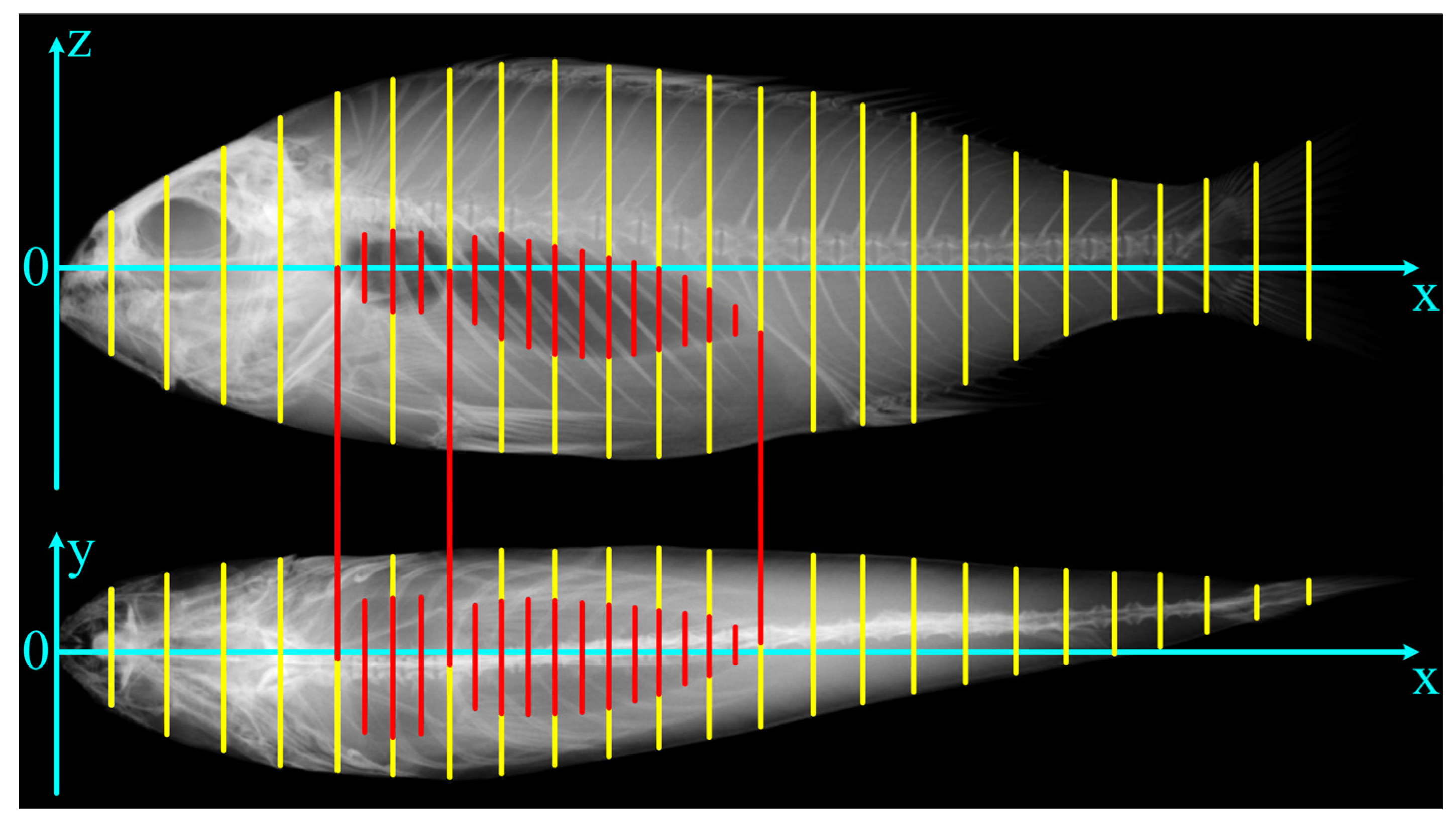
The samples with ice-water mixture were transferred to the laboratory within 24 h to minimize any changes in their body and swim bladder shape. Before recording the body length and body weight, each captured individual was radiographed in both the lateral and dorsoventral orientations. A state-of-the-art X-ray imaging system (SOFTEX M-100) was adopted to trace the outlines of fish body and swim bladder of each sample, with the input voltage of AC 200 V and the maximum tube voltage of 100 kV. Morphological parameters from 19 individuals were measured and recorded as shown in Figure 1, for facilitating the spatial reconstruction of fish body and swim bladder and TS modelling.
2.3. TS Model Calculation and Estimation
The acoustic backscatter of T. jarbua was modelled utilizing the spatial three-dimensional fish body and swim bladder shapes. The KRM model approximates every scattering individual as an adjacent series of finite cylinders to characterize the acoustic properties of each captured sample. The swim bladder was regarded as a set of gas-filled cylinders surrounded by the fish body, which can be treated as a range of fluid-filled cylinder sections. Total fish TS was formulated as the coherent sum of both fish body and swim bladder cylindrical elements.
Due to the TS calculation demands of the KRM model, typical parameters are provided in Table 1 [36]. The critical acoustic parameters including the density contrast and sound velocity contrast can be calculated by the above parameters. Since the TS of T. jarbua is extremely correlated with acoustic frequency as well as the pitch angle, the selections of both acoustic frequency and pitch angle distribution are considerable. Referring to the common frequencies used in the UWA investigation of offshore fisheries resources in the South China Sea, four types of frequencies of 38 kHz, 70 kHz, 120 kHz, and 200 kHz were determined for TS estimation. Meanwhile, the pitch angle ranged from −50° to 50° was adopted to calculate the TS variations on the premise that the pitch angle was defined as 0° while the incident sound wave was perpendicular to the dorsal aspect of fish body [42].
The evaluated TS across the pitch angle distribution was applied to compute the average TS, which represented the TS of individual T. jarbua. Note that the pitch angle follows a normal distribution, and two classic pitch angle distributions that include and are adopted to calculate the average TS of T. jarbua [34]. As total fish TS can be treated as the coherent sum of both fish body and swim bladder cylindrical elements, the average TS of T. jarbua was calculated as follows [36].
The scattering length of swim bladder can be formulated as [36]
where and are the reflection coefficients at the fish body-swim bladder interface and the fish body-seawater interface, respectively. is the number of swim bladder segments, and represents empirical amplitude. denotes the sound wave number inside the fish body, and is the equivalent radius of cylinder. is the angle from the horizontal axis to the axis of cylinder, denotes the empirical phase adjustment, and represents the projection of slice on the horizontal axis in the rotated coordinates.
The scattering length of fish body can be expressed as [36]
where is the number of fish body segments, and denotes the sound wave number in the water. and are the coordinates of the upper and lower surfaces of the cylinder, respectively. is the transmission coefficient of sound wave incidence from the seawater to the fish body, denotes the transmission coefficient of sound wave incidence from the fish body to the seawater, and represents an empirical phase correction.
The total scattering length can be treated as a coherent summation, hence, the total backscattering cross section can be written as
Accordingly, the TS of fish can be expressed as
The relationship between TS and L was analyzed and summarized to derive a regression equation utilizing the least-squares approach, which can be formulated as
where is the slope of regression equation, and b denotes the intercept. Let , Equation (5) can be rewritten as
where represents the intercept while , and Equation (6) is also known as a standard form.
3. Results
3.1. Biological Sampling and Measurement
A total of 19 T. jarbua were caught to facilitate the TS calculation, and the detailed morphological parameters are provided in Table 2. From Table 2 we can notice that the body length range of 19 T. jarbua was distributed from 9.97 cm to 20.52 cm, with an average of 16.14 cm. The body weight range of all samples was 26.5 g to 240.3 g, with an average of 129.7 g. In conclusion, the regression relationship between W and L can be determined through the least-squares method as shown in Figure 2.
From Figure 2, we can conclude that the W-L regression equation could be fitted as , where the 95% confidence intervals of its fitted coefficients are [0.005129 0.07307] and [2.580 3.178], respectively. Moreover, indicates that there exists the excellent goodness of fit between the factual data and the fitted curve.
3.2. TS Variation with Pitch Angle
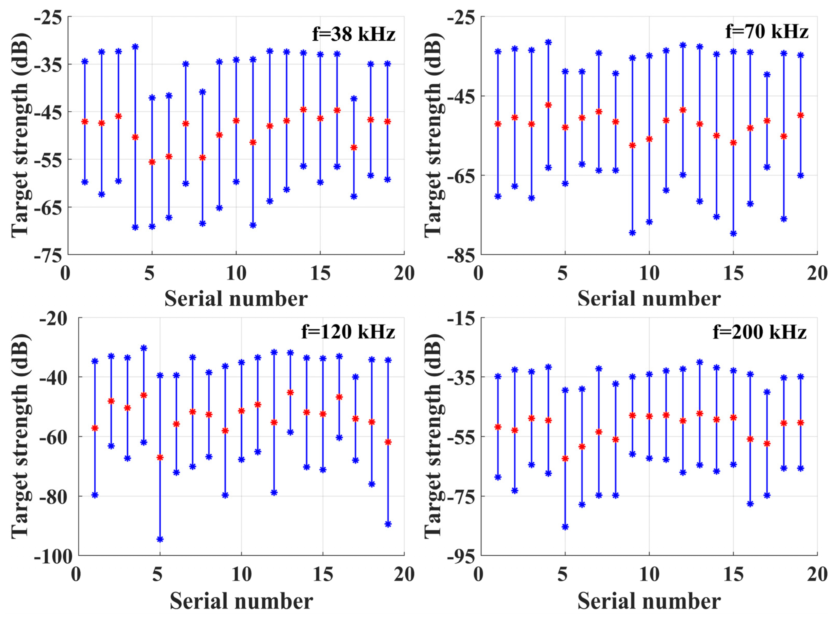
The spatial structure coordinate parameters of the fish body and swim bladder were acquired and established by measuring the X-ray images of all the samples. Then these parameters were used to calculate the TS with the pitch angles ranging from −50° to 50°. Let denote the TS variational scale, the scopes of the 19 T. jarbua at four frequencies are provided in Figure 3. From Figure 3, we can see that the scopes at four types of frequencies of 38 kHz, 70 kHz, 120 kHz, and 200 kHz were 20.51–37.85 dB, 23.27–45.77 dB, 26.65–55.01 dB and 25.85–45.86 dB, respectively.
As a particular analysis, the TS variation with respect to fish body, swim bladder and the whole fish (L = 16.01 cm) corresponding to the pitch angle transformations are provided in Figure 4. From Figure 4, we can notice that the TS variation of the whole fish is primarily consistent with that of the swim bladder other than the fish body regardless of the frequencies, which indicates that the swim bladder is the dominant component of acoustic backscattering in the whole fish.
The TS characteristics of T. jarbua were significantly affected by the pitch angle and exhibited a multimodal distribution. Moreover, the frequency was also a considerable element that affects the TS features. At four types of frequencies of 38 kHz, 70 kHz, 120 kHz, and 200 kHz, the dominant TS peaks were located at the pitch angle of about −15° to −5°. As the frequency increased, the number of secondary TS peaks also increased gradually. These results indicated that the influence of fish posture corresponding to the fish behavior on TS would be enhanced with increasing frequency.
3.3. TS Variation with Body Length
The average TS of each specimen corresponding to the different pitch angle distributions at 38 kHz, 70 kHz, 120 kHz, and 200 kHz were investigated and calculated to ultimately formulate the TS-L equation. At the same frequency, the differences in average TS between the individuals with the maximum and minimum body length at the two pitch angle distributions were not less than 1 dB, which increased as the increasing frequency.
Moreover, the average TS of all samples with respect to the two pitch angle distributions at 38 kHz, 70 kHz, 120 kHz, and 200 kHz are provided in Table 3. From Table 3, we can see that the differences in average TS between two pitch angle distributions at the same frequency do not exceed 0.3 dB. For the same pitch angle distribution, the maximum difference in average TS between different frequencies was about 2 dB.
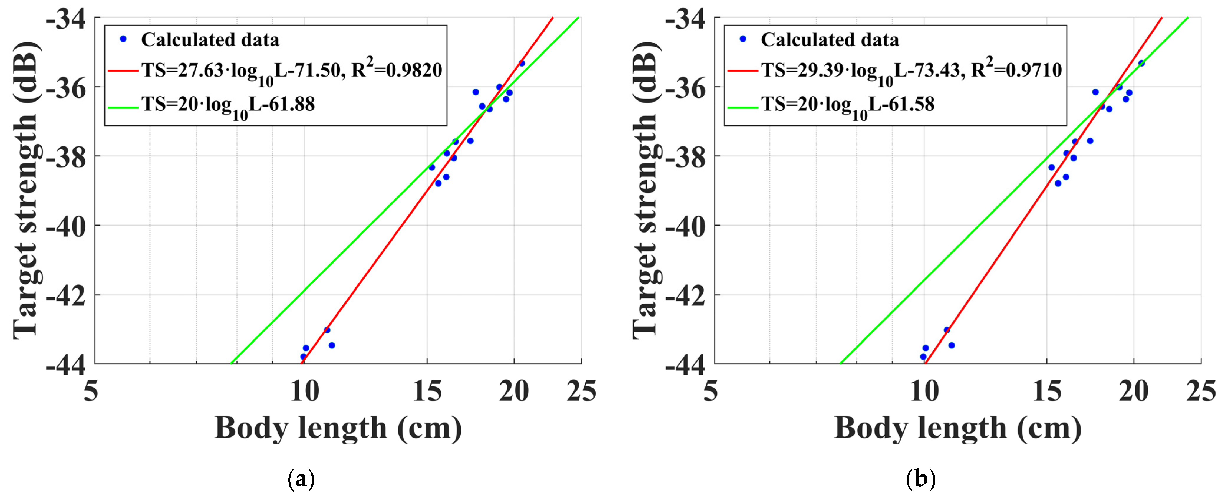
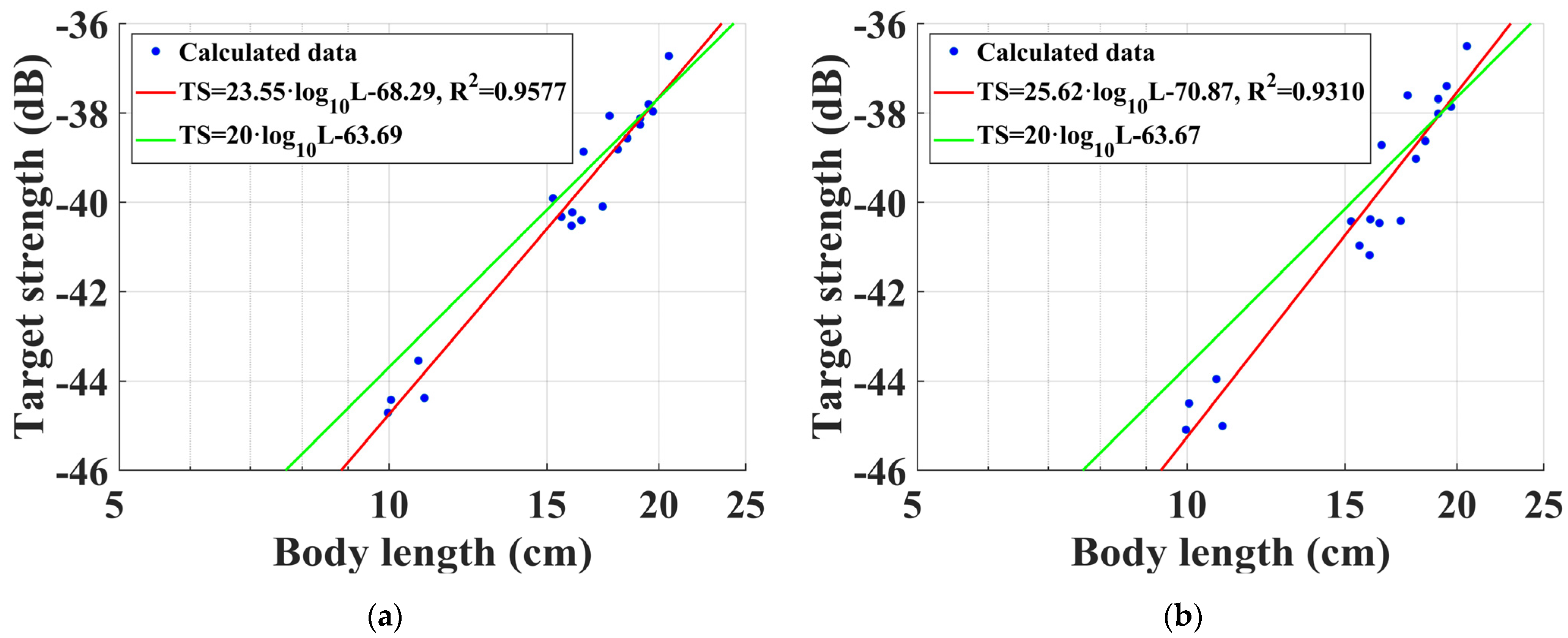
After analyzing the TS characteristics of T. jarbua, a crucial objective was to acquire the TS-L equation using the least-squares algorithm. The relationships between TS and body length for different pitch angle distributions at four types of frequencies of 38 kHz, 70 kHz, 120 kHz, and 200 kHz are displayed in Figure 5, Figure 6, Figure 7 and Figure 8. Furthermore, the fitted TS-L regression formulations as well as the standard form equations are listed in Table 4.
From Figure 5, Figure 6, Figure 7 and Figure 8, we can conclude that TS increases with the increasing body length at different pitch angle distributions and frequencies. The fitted TS-L regression equations generally exhibited a difference from the standard equations with the form. For four frequencies, the R-squared values of the fitted TS-L regression equations at were larger than those at , which might be caused by the fact that the activity habits of T. jarbua were in line with the .
As displayed in Table 4, when , the corresponding first decreased and then slightly increased as the frequency increased. Accordingly, the TS reached the maximum at 38 kHz and the minimum at 120 kHz in the same pitch angle distribution. The values for the two pitch angle distributions at the same frequency almost differed by less than 0.3 dB.
4. Discussion
The premise of TS calculation using the KRM model is to accurately measure and record the particular morphological parameters of fish body and swim bladder for constructing the three-dimensional spatial coordinate of T. jarbua. Hence, a state-of-the-art X-ray imaging system with a resolution of 0.01 mm was adopted to generate a X-ray image for tracing the outlines of fish body and swim bladder of each individual, which could authentically and precisely reflect the internal structure of the whole fish.
The freshness quality of samples significantly affected by the storage and transportation conditions resulted in the swim bladder structure might be deformed or even damaged, so not each X-ray image could be adopted to calculate the TS of T. jarbua. In this study, all samples were collected by a midwater trawl in situ and stored on the ice-water mixture in an insulated box for ensuring its relative integrality of the biological structure of T. jarbua. Different from freezing and then thawing, the samples were transferred to the laboratory and completed for X-ray photography within 24 h, which minimized any changes in their body and swim bladder shape to improve the measurement accuracy of morphological parameters. It is desirable to implement in situ X-ray photography to avoid the effects of storage and transportation on fish samples.
The TS of T. jarbua is affected by many factors, one of which is the frequency of the sound wave [37]. In the low frequency case of 38 kHz, the TS variation with the pitch angle exhibited a relatively stable state, with a dominant peak and a small number of secondary peaks. The interaction between sound waves in the fish generated more interference at the high frequency conditions, leading to more secondary peaks. Therefore, we can conclude that the low frequency is more suitable for the abundance estimation of T. jarbua since its TS was sensitive to the pitch angle at high frequencies. In fact, 38 kHz is also used as a main frequency in the offshore fisheries resources assessment in the South China Sea.
Another significant factor affecting the TS of T. jarbua is the pitch angle, which is related to the individual size, swimming posture as well as living conditions [39]. In this study, two classic types of pitch angle distributions were adopted to calculate the average TS of T. jarbua [34]. At the same frequency, there was almost no difference in the average TS calculated for the two pitch angle distributions, which indicated that the pitch angle distribution had little effects on the TS of T. jarbua using the KRM. A more reasonable approach is to use an optical camera to record and investigate the actual pitch angle distribution, for computing the average TS of T. jarbua.
T. jarbua is a type of fish with a two-chamber swim bladder, which is filled with gas. It has been reported that the swim bladder contribution approximately accounts for 90–95% of the overall acoustic backscattering of the whole fish and determines the magnitude of the TS [43]. Therefore, those factors that can significantly affect the shape and size of the swim bladder, such as stomach fullness, the development degree of gonadal as well as the living water layer, have become considerable reasons for the scale of TS. It is also necessary to implement comprehensive research on the TS variations with the physiological characteristics of T. jarbua.
5. Conclusions
Effective UWA surveys on the biomass require comprehensive knowledge of the TS characteristics of T. jarbua. In this study, the KRM model was adopted to investigate and evaluate the influences of morphological characteristics on the acoustic TS of T. jarbua in the South China Sea, in order to improve the accuracy and reliability of acoustic abundance assessment. A total of 19 individuals were captured and applied to estimate and analyze the TS variations of T. jarbua with the sound wave frequency, pitch angle distribution as well as body length. The results indicated that the TS of T. jarbua varied with the pitch angle shifts, and the number of secondary TS peaks increased as the increasing frequency accordingly. At four types of frequencies of 38 kHz, 70 kHz, 120 kHz, and 200 kHz, the dominant TS peaks were located at the pitch angle of about −15° to −5°. The fitted TS-L regression equations as well as the standard b20 form formulations were determined at different pitch angle distributions and frequencies. These findings could provide significant references for the accurate and reliable acoustic abundance estimation in the South China Sea, facilitating a better understanding of the population dynamics of T. jarbua.
Author Contributions
Conceptualization, B.L. and J.L.; methodology, B.L.; software, X.G.; validation, B.L., J.L. and X.G.; formal analysis, F.W.; investigation, Z.H.; resources, B.L.; data curation, B.L.; writing—original draft preparation, B.L.; writing—review and editing, H.H.; visualization, F.W.; supervision, H.H.; project administration, X.G.; funding acquisition, B.L., X.G. and H.H. All authors have read and agreed to the published version of the manuscript.
Funding
This research was funded by the Research Start-up Funding of Fujian University of Technology, grant numbers GY-Z220198 and GY-Z23027, the Fujian Provincial Department of Science and Technology Announces Major Special Projects, grant number 2023HZ025003, and the Key Scientific and Technological Innovation Projects of Fujian Province, grant number 2023XQ015. The APC was funded by the Fujian Provincial Department of Science and Technology Announces Major Special Projects, grant number 2023HZ025003.
Data Availability Statement
The data presented in this study are available on request from the corresponding author. As the data are a part of an ongoing study, the data are not publicly available.
Conflicts of Interest
The authors declare no conflicts of interest.
References
- Chien, L.T.; Hwang, D.F.; Jeng, S.S. Effect of Thermal Stress on Dietary Requirement of Vitamin C in Thornfish Terapon jarbua. Fish. Sci. 1999, 65, 731–735. [Google Scholar] [CrossRef]
- Koslow, J.A. The Role of Acoustics in Ecosystem-Based Fishery Management. ICES J. Mar. Sci. 2009, 66, 966–973. [Google Scholar] [CrossRef]
- Davison, P.C.; Koslow, J.A.; Kloser, R.J. Acoustic Biomass Estimation of Mesopelagic Fish: Backscattering from Individuals, Populations, and Communities. ICES J. Mar. Sci. 2015, 72, 1413–1424. [Google Scholar] [CrossRef]
- Deshpande, K.; Kelkar, N. Acoustic Identification of Otomops wroughtoni and Other Free-Tailed Bat Species (Chiroptera: Molossidae) from India. Acta Chiropterol. 2015, 17, 419–428. [Google Scholar] [CrossRef]
- Korneliussen, R.J. The Acoustic Identification of Atlantic Mackerel. ICES J. Mar. Sci. 2010, 67, 1749–1758. [Google Scholar] [CrossRef]
- Tan, X.; Kang, M.; Tao, J.; Li, X.; Huang, D. Hydroacoustics Survey of Fish Density, Spatial Distribution, and Behavior Upstream and Downstream of the Changzhou Dam on the Pearl River, China. Fish. Sci. 2011, 77, 891–901. [Google Scholar] [CrossRef]
- Foote, K.G. Fish Target Strengths for Use in Echo Integrator Surveys. J. Acoust. Soc. Am. 1987, 82, 981–987. [Google Scholar] [CrossRef]
- Simmonds, E.J.; MacLennan, D.N. Fisheries Acoustics: Theory and Practice, 2nd ed.; Blackwell Publishing Science: Oxford, UK, 2005; pp. 1–437. ISBN 9780632059942. [Google Scholar]
- Doray, M.; Josse, E.; Gervain, P.; Reynal, L.; Chantrel, J. Acoustic Characterization of Pelagic Fish Aggregations around Moored Fish Aggregating Devices in Martinique (Lesser antilles). Fish. Res. 2006, 82, 162–175. [Google Scholar] [CrossRef]
- Barange, M. Acoustic Identification, Classification and Structure of Biological Patchiness on the Edge of the Agulhas Bank and Its Relation to Frontal Features. S. Afr. J. Mar. Sci. 1994, 14, 333–347. [Google Scholar] [CrossRef]
- Bernasconi, M.; Patel, R.; Nøttestad, L.; Pedersen, G.; Brierley, A.S. The Effect of Depth on the Target Strength of A Humpback Whale (Megaptera novaeangliae). J. Acoust. Soc. Am. 2013, 134, 4316–4322. [Google Scholar] [CrossRef]
- Mukai, T.; Lida, K. Depth Dependence of Target Strength of Live Kokanee Salmon in Accordance with Boyle’s Law. ICES J. Mar. Sci. 1996, 53, 245–248. [Google Scholar] [CrossRef]
- Sobradillo, B.; Boyra, G.; Pérez-Arjona, I.; Martinez, U.; Espinosa, V. Ex Situ and In Situ Target Strength Measurements of European Anchovy in the Bay of Biscay. ICES J. Mar. Sci. 2021, 78, 782–796. [Google Scholar] [CrossRef]
- Zhao, X.; Wang, Y.; Dai, F. Depth-Dependent Target Strength of Anchovy (Engraulis japonicus) Measured In Situ. ICES J. Mar. Sci. 2008, 65, 882–888. [Google Scholar] [CrossRef]
- Sawada, K.; Takahashi, H.; Abe, K.; Ichii, T.; Watanabe, K.; Takao, Y. Target-Strength, Length, and Tilt-Angle Measurements of Pacific Saury (Cololabis saira) and Japanese Anchovy (Engraulis japonicus) Using an Acoustic-Optical System. ICES J. Mar. Sci. 2009, 66, 1212–1218. [Google Scholar] [CrossRef]
- Salvetat, J.; Lebourges-Dhaussy, A.; Travassos, P.; Gastauer, S.; Roudaut, G.; Vargas, G.; Bertrand, A. Corrigendum to: In Situ Target Strength Measurement of the Black Triggerfish Melichthys niger and the Ocean Triggerfish Canthidermis sufflamen. Mar. Freshw. Res. 2021, 72, 449. [Google Scholar] [CrossRef]
- Robertis, A.D.; Taylor, K. In Situ Target Strength Measurements of the Scyphomedusa Chrysaora melanaster. Fish. Res. 2014, 153, 18–23. [Google Scholar] [CrossRef]
- Murase, H.; Kawabata, A.; Kubota, H.; Nakagami, M.; Amakasu, K.; Abe, K.; Miyashita, K. Effect of Depth-Dependent Target Strength on Biomass Estimation of Japanese Anchovy. J. Mar. Sci. Tech. 2011, 19, 267–272. [Google Scholar] [CrossRef]
- Fernandes, P.G.; Copland, P.; Garcoa, R.; Nicosevici, T.; Scoulding, B. Additional Evidence for Fisheries Acoustics: Small Cameras and Angling Gear Provide Tilt Angle Distributions and Other Relevant Data for Mackerel Surveys. ICES J. Mar. Sci. 2016, 73, 2009–2019. [Google Scholar] [CrossRef]
- Glass, C. Dynamics of Pelagic Fish Distribution and Behaviour: Effect on Fisheries and Stock Assessment. Pierre Fréeon and Ole Arve Misund. Rev. Fish. Biol. Fisher. 2000, 10, 124. [Google Scholar] [CrossRef]
- Peltonen, H.; Balk, H. The Acoustic Target Strength of Herring (Clupea harengus L.) in the Northern Baltic Sea. ICES J. Mar. Sci. 2005, 62, 803–808. [Google Scholar] [CrossRef]
- Zhang, J.; Chen, Z.; Chen, G.; Zhang, P.; Qiu, Y.; Yao, Z. Hydroacoustic Studies on the Commercially Important Squid Sthenoteuthis Oualaniensis in the South China Sea. Fish. Res. 2015, 169, 45–51. [Google Scholar] [CrossRef]
- Kang, D.; Hwang, D. Ex Situ Target Strength of Rockfish (Sebastes schlegeli) and Red Sea Bream (Pagrus major) in the Northwest Pacific. ICES J. Mar. Sci. 2003, 60, 538–543. [Google Scholar] [CrossRef]
- Rodríguez-Sánchez, V.; Encina-Encina, L.; Rodríguez-Ruiz, A.; Sánchez-Carmona, R. Horizontal Target Strength of Luciobarbus sp. in Ex Situ Experiments: Testing Differences by Aspect Angle, Pulse Length and Beam Position. Fish. Res. 2015, 164, 214–222. [Google Scholar] [CrossRef]
- Kang, D.; Cho, S.; Lee, C.; Myoung, J.; Na, J. Ex Situ Target-Strength Measurements of Japanese Anchovy (Engraulis japonicus) in the Coastal Northwest Pacific. ICES J. Mar. Sci. 2009, 66, 1219–1224. [Google Scholar] [CrossRef]
- Kim, H.; Cho, S.; Kim, M.; Kim, S.; Kang, D. Acoustic Target Strength According to Different Growth Stages of Japanese Anchovy (Engraulis japonicus): A Comparison of Juvenile and Adult Fish. J. Mar. Sci. Eng. 2023, 11, 1575. [Google Scholar] [CrossRef]
- Chen, G.; Li, Y.; Chen, P.; Zhang, J.; Fang, L.; Li, N. Measurement of Single-Fish Target Strength in the South China Sea. Chin. J. Oceanol. Limn. 2012, 30, 554–562. [Google Scholar] [CrossRef]
- Chu, D.; Eastland, G.C. Calibration of a Broadband Acoustic Transducer with a Standard Spherical Target in the Near Field. J. Acoust. Soc. Am. 2015, 137, 2148–2157. [Google Scholar] [CrossRef]
- Foote, K.G. Discriminating between the Nearfield and the Farfield of Acoustic Transducers. J. Acoust. Soc. Am. 2014, 136, 1511–1517. [Google Scholar] [CrossRef]
- Hazen, L.E.; Horne, J.K. A Method for Evaluating the Effects of Biological Factors on Fish Target Strength. ICES J. Mar. Sci. 2003, 60, 555–562. [Google Scholar] [CrossRef]
- Khodabandeloo, B.; Agersted, M.D.; Klevjer, T.; Macaulay, G.J.; Melle, W. Estimating Target Strength and Physical Characteristics of Gas-Bearing Mesopelagic Fish from Wideband In Situ Echoes using a Viscous-Elastic Scattering Model. J. Acoust. Soc. Am. 2021, 149, 673–691. [Google Scholar] [CrossRef] [PubMed]
- Jech, J.M.; Horne, J.K. Three-Dimensional Visualization of Fish Morphometry and Acoustic Backscatter. Acoust. Res. Lett. 2002, 3, 35–40. [Google Scholar] [CrossRef]
- Tang, Y.; Nishimori, Y.; Furusawa, M. The Average Three-Dimensional Target Strength of Fish by Spheroid Model for Sonar Surveys. ICES J. Mar. Sci. 2009, 66, 1176–1183. [Google Scholar] [CrossRef]
- Furusawa, M. Prolate Spheroidal Models for Predicting General Trends of Fish Target Strength. J. Acoust. Soc. Jpn. 1988, 9, 13–24. [Google Scholar] [CrossRef]
- Stanton, T.K. Sound Scattering by Cylinders of Finite Length. III. Deformed Cylinders. J. Acoust. Soc. Am. 1989, 86, 691–705. [Google Scholar] [CrossRef]
- Clay, C.S.; Horne, J.K. Acoustic Models of Fish: The Atlantic Cod (Gadus Morhua). J. Acoust. Soc. Am. 1994, 96, 1661–1668. [Google Scholar] [CrossRef]
- Gauthier, S.; Horne, J.K. Acoustic Characteristics of Forage Fish Species in the Gulf of Alaska and Bering Sea Based on Kirchhoff-Approximation Models. Can. J. Fish. Aquat. Sci. 2004, 61, 1839–1850. [Google Scholar] [CrossRef]
- Horne, J.K. The Influence of Ontogeny, Physiology, and Behaviour on the Target Strength of Walleye Pollock (Theragra chalcogramma). ICES J. Mar. Sci. 2003, 60, 1063–1074. [Google Scholar] [CrossRef]
- Tong, J.; Xue, M.; Zhu, Z.; Wang, W.; Tian, S. Impacts of Morphological Characteristics on Target Strength of Chub Mackerel (Scomber japonicus) in the Northwest Pacific Ocean. Front. Mar. Sci. 2022, 9, 856483. [Google Scholar] [CrossRef]
- Kusdinar, A.; Hwang, B.K.; Shin, H.O. Determining the Target Strength Bambood Wrasse (Pseudolabrus japonicus) Using Kirchhoff-Ray Mode. J. Kor. Soc. Fish. Technol. 2014, 50, 427–434. [Google Scholar] [CrossRef]
- Kang, D.; Sadayasu, K.; Mukai, S.; Lida, K.; Hwang, D.; Sawada, K.; Miyashita, K. Target Strength Estimation of Black Porgy Acanthopagrus Schlegeli Using Acoustic Measurements and A Scattering Model. Fish. Sci. 2004, 70, 819–828. [Google Scholar] [CrossRef]
- Love, R.H. Dorsal-aspect Target Strength of an Individual Fish. J. Acoust. Soc. Am. 1971, 49, 816–823. [Google Scholar] [CrossRef]
- Foote, K.G. Importance of the Swimbladder in Acoustic Scattering by Fish: A Comparison of Gadoid and Mackerel Target Strength. J. Acoust. Soc. Am. 1980, 67, 2084–2089. [Google Scholar] [CrossRef]
Figure 1.
Geometric construction of lateral and dorsoventral X-ray images. The air-filled swim bladder can be regarded as a black shape in the fish body. The definition of the morphological parameters of the fish body and swim bladder used to calculate the TS can be referred to [40].
Figure 1.
Geometric construction of lateral and dorsoventral X-ray images. The air-filled swim bladder can be regarded as a black shape in the fish body. The definition of the morphological parameters of the fish body and swim bladder used to calculate the TS can be referred to [40].

Figure 2.
The regression equation of body weight of T. jarbua with body length.

Figure 3.
TS scales of every individual with respect to the pitch angle ranging from −50° to 50°. Note that the blue points located at the top and bottom endpoints of the vertical lines are the maximum and minimum values of TS, respectively. The red middle point represents the half of .
Figure 3.
TS scales of every individual with respect to the pitch angle ranging from −50° to 50°. Note that the blue points located at the top and bottom endpoints of the vertical lines are the maximum and minimum values of TS, respectively. The red middle point represents the half of .

Figure 4.
TS variation of fish body, swim bladder and the whole fish (L = 16.01 cm) corresponding to the pitch angle transformations at four types of frequencies of 38 kHz, 70 kHz, 120 kHz, and 200 kHz.
Figure 4.
TS variation of fish body, swim bladder and the whole fish (L = 16.01 cm) corresponding to the pitch angle transformations at four types of frequencies of 38 kHz, 70 kHz, 120 kHz, and 200 kHz.

Figure 5.
TS variation of T. jarbua with body length calculated using the two pitch angle distributions at 38 kHz. (a) TS variation with body length at ; (b) TS variation with body length at .
Figure 5.
TS variation of T. jarbua with body length calculated using the two pitch angle distributions at 38 kHz. (a) TS variation with body length at ; (b) TS variation with body length at .

Figure 6.
TS variation of T. jarbua with body length calculated using the two pitch angle distributions at 70 kHz. (a) TS variation with body length at ; (b) TS variation with body length at .
Figure 6.
TS variation of T. jarbua with body length calculated using the two pitch angle distributions at 70 kHz. (a) TS variation with body length at ; (b) TS variation with body length at .

Figure 7.
TS variation of T. jarbua with body length calculated using the two pitch angle distributions at 120 kHz. (a) TS variation with body length at ; (b) TS variation with body length at .
Figure 7.
TS variation of T. jarbua with body length calculated using the two pitch angle distributions at 120 kHz. (a) TS variation with body length at ; (b) TS variation with body length at .

Figure 8.
TS variation of T. jarbua with body length calculated using the two pitch angle distributions at 200 kHz. (a) TS variation with body length at ; (b) TS variation with body length at .
Figure 8.
TS variation of T. jarbua with body length calculated using the two pitch angle distributions at 200 kHz. (a) TS variation with body length at ; (b) TS variation with body length at .


Table 1.
Typical parameters used in the KRM model.
| Medium | Sound Velocity (m/s) |
|---|---|
| Sound velocity in seawater (m/s) | 1490 |
| Sound velocity in fish body (m/s) | 1570 |
| Sound velocity in swim bladder (m/s) | 345 |
| Density of seawater (kg/m3) | 1030 |
| Density of fish body (kg/m3) | 1070 |
| Density of swim bladder (kg/m3) | 1.24 |
Table 2.
Morphological parameters of T. jarbua samples.
| Serial Number | Body Length (cm) | Body Weight (g) |
|---|---|---|
| 1 | 16.01 | 133.4 |
| 2 | 19.06 | 181.1 |
| 3 | 19.06 | 174.5 |
| 4 | 20.52 | 240.3 |
| 5 | 10.05 | 30.0 |
| 6 | 10.95 | 33.3 |
| 7 | 15.24 | 109.5 |
| 8 | 10.78 | 35.0 |
| 9 | 16.39 | 125.3 |
| 10 | 17.31 | 130.5 |
| 11 | 16.48 | 119.6 |
| 12 | 17.62 | 154.1 |
| 13 | 19.70 | 200.2 |
| 14 | 19.48 | 213.3 |
| 15 | 18.44 | 177.5 |
| 16 | 18.00 | 171.1 |
| 17 | 9.97 | 26.5 |
| 18 | 15.98 | 108.0 |
| 19 | 15.57 | 100.5 |
Table 3.
Average TS of two pitch angle distributions at four types of frequencies of 38 kHz, 70 kHz, 120 kHz, and 200 kHz.
Table 3.
Average TS of two pitch angle distributions at four types of frequencies of 38 kHz, 70 kHz, 120 kHz, and 200 kHz.
| Pitch Angle Distribution | Frequency (kHz) | Average TS (dB) |
|---|---|---|
| 38 | −37.72 | |
| 70 | −38.86 | |
| 120 | −39.63 | |
| 200 | −39.53 | |
| 38 | −37.42 | |
| 70 | −38.70 | |
| 120 | −39.72 | |
| 200 | −39.51 |
Table 4.
The regression equations as well as standard b20 form equations of T. jarbua for two pitch angle distributions at 38 kHz, 70 kHz, 120 kHz, and 200 kHz.
Table 4.
The regression equations as well as standard b20 form equations of T. jarbua for two pitch angle distributions at 38 kHz, 70 kHz, 120 kHz, and 200 kHz.
| Pitch Angle Distribution | Frequency (kHz) | Regression Equation | Standard b20 Form Equation |
|---|---|---|---|
| 38 | |||
| 70 | |||
| 120 | |||
| 200 | |||
| 38 | |||
| 70 | |||
| 120 | |||
| 200 |
Disclaimer/Publisher’s Note: The statements, opinions and data contained in all publications are solely those of the individual author(s) and contributor(s) and not of MDPI and/or the editor(s). MDPI and/or the editor(s) disclaim responsibility for any injury to people or property resulting from any ideas, methods, instructions or products referred to in the content. |
© 2024 by the authors. Licensee MDPI, Basel, Switzerland. This article is an open access article distributed under the terms and conditions of the Creative Commons Attribution (CC BY) license (https://creativecommons.org/licenses/by/4.0/).
Share and Cite
MDPI and ACS Style
Li, B.; Liu, J.; Gao, X.; Huang, H.; Wang, F.; Huang, Z. Acoustic Target Strength of Thornfish (Terapon jarbua) Based on the Kirchhoff-Ray Mode Model. Electronics 2024, 13, 1279. https://0-doi-org.brum.beds.ac.uk/10.3390/electronics13071279
AMA Style
Li B, Liu J, Gao X, Huang H, Wang F, Huang Z. Acoustic Target Strength of Thornfish (Terapon jarbua) Based on the Kirchhoff-Ray Mode Model. Electronics. 2024; 13(7):1279. https://0-doi-org.brum.beds.ac.uk/10.3390/electronics13071279
Chicago/Turabian StyleLi, Bin, Jiahao Liu, Xiujing Gao, Hongwu Huang, Fang Wang, and Zhuoya Huang. 2024. "Acoustic Target Strength of Thornfish (Terapon jarbua) Based on the Kirchhoff-Ray Mode Model" Electronics 13, no. 7: 1279. https://0-doi-org.brum.beds.ac.uk/10.3390/electronics13071279
Note that from the first issue of 2016, this journal uses article numbers instead of page numbers. See further details here.