1. Introduction
With the rapid advancement of science and technology, increasing attention is being drawn to intelligent navigation technology for ships in the domains of maritime and marine technology. Although progress has been made, challenges still exist [
1]. Extensive research has been conducted by scholars worldwide on local path planning, which is a critical component of ship intelligent navigation. It involves the analysis and consideration of various environmental information and influencing factors. Difficulties arise in predicting the behavior of interfering ships due to ambiguous descriptions in the International Regulations for Preventing Collisions at Sea (COLREGS), such as “seafarers’ usual practice” and “good seamanship”. As a result, ensuring safe autonomous navigation necessitates addressing various issues in the ship’s local path planning process. Included in these considerations is the design of a path that conforms to the COLREGS, which involves incorporating information on the multiple interfering ships and static obstacles while ensuring effectiveness. Furthermore, it is crucial to scientifically and effectively validate the reliability of the ship’s local path.
Representative studies on the ship’s local path planning are mainly as follows:
To achieve local path optimization for unmanned ships, Almeida et al. [
2] employed an onboard video acquisition system to obtain environmental information, construct a map, and assess the danger level based on the distance between the unmanned ship and obstacles. A real-time path planning algorithm for surface unmanned vehicles (USVs) considering angular rate constraints was proposed by Kim et al. [
3], and the steering performance of the ship was taken into account. To solve the problem of heading constraint faced by USV during actual navigation, a course-angle-oriented fast-traveling square algorithm (AFMS) was proposed by Liu and Bucknall [
4]. In an unknown environment, to achieve dynamic path planning, the wind-driven optimization algorithm was utilized by Pandey and Parhi [
5] to optimize and adjust the parameters of the fuzzy controller’s input/output membership function. A multi-layer fast-travel path planning algorithm was proposed by Song et al. [
6] for the real-time generation of a USV trajectory in dynamic environments. The planning spatial information and sea surface current information are considered comprehensively. A path-planning method for multiple moving targets in complex water navigation environments was introduced by Du et al. [
7]. The method entails the utilization of complex map construction, employing the complexity theory. Furthermore, the A* algorithm is combined with the constructed map to generate an optimal path that minimizes the travel distance and prevents local minima. An approach for optimal path selection in ship navigation, aimed at ensuring ship stability, was proposed by Krata and Szlapczynska [
8]. In this approach, the method of equivalent eccentric height is employed to simulate waves’ natural rolling period, establishing the resonant motion of ships as the basis for dynamic path optimization. Ship collision avoidance was transformed into an optimal control problem by Kozynchenko et al. [
9]. They formulated a nonlinear three-dimensional ship dynamic motion model and validated the efficacy of the proposed method in a two-ship intersection scenario. A ship’s path optimization method based on three-dimensional dynamic programming was proposed by Zaccone et al. [
10]. The method incorporates meteorological conditions and takes into account the ship’s motion performance and the resistance caused by waves. It parameterizes the sailing process into a multi-stage decision-making process, calculates the seaworthiness of each segment, and enables dynamic path planning. The velocity barrier method was combined with an enhanced artificial potential field algorithm by Song et al. [
11]. They established the velocity vector relationship between the ship and the obstacle by generating a complex potential field around the obstacle. The collision between the ship and the obstacle was prevented by utilizing the repulsive and centrifugal potential fields. Ma et al. [
12] took the influence of obstacles and ocean currents into consideration, transformed the path planning problem of USVs into a problem about multi-objective nonlinear optimization, which is constrained by collision avoidance, moving boundary and speed, and sought the optimal path length, smoothness, economy, and safety, and solved it. Song et al. [
13] proposed an improved A* algorithm. Three path-smoothing devices are used to smooth the path. The performance of the improved A* algorithm is compared with the performance of the traditional A* algorithm.
In recent years, by reviewing the existing commonly used research methods and classical algorithms, and based on multi-modal constraints, the path planning research was divided by Zhou et al. [
14] into three aspects: path planning, motion planning, and trajectory planning. The problems in existing research were analyzed, and suggestions for future research were put forward. Yan et al. [
15] proposed a path-planning method based on anisotropic Fast Marching. The method combines a repulsive force field and joint potential field to estimate the navigation cost, and optimizes the path using expert knowledge to effectively avoid dynamic and static obstacles. The simulation results demonstrate the method’s effectiveness in path planning for busy waters. Vagale et al. [
16] examined the current research on the path-planning of unmanned ships and introduced a Guidance, Navigation, and Control (GNC) algorithm. A local path optimization method for unmanned ships was proposed by Wang et al. [
17] based on particle swarm optimization (PSO) calculation and dynamic optimal control to ensure the dynamic optimization of the cruise path of unmanned ships under time-varying conditions. A multi-subjective artificial potential field algorithm was proposed by Sang et al. [
18] to enhance the conventional method for local path planning of unmanned vehicle formation. This algorithm ensures path continuity and smoothness while considering the dynamic characteristics of unmanned vehicles. A method based on Deep Reinforcement Learning (DRL) and Artificial Potential Field (APF) algorithms was proposed by Li et al. [
19], and it is pointed out that in future work, the influence of uncertain environmental factors should be considered. A path planning method was proposed by Krell et al. [
20] combining PSO and a visibility graph, and optimized the path according to energy efficiency and reward function. An improved BA* algorithm for the path planning of unmanned surface ships in coverage scenarios was proposed by Ma et al. [
21]. The algorithm’s benefits in terms of the path length, number of turns, units, and coverage were experimentally verified. A method for multi-ship swarm path planning based on local sensor information was proposed by Wang et al. [
22], achieving collision-free, smooth, and dynamically feasible path generation through dynamic path search and B-spline curve optimization. Yang et al. [
23] improved the A* algorithm based on the artificial potential field method to consider the influence of ocean currents and static obstacles on path planning, and smoothed the generated paths. Given the focus on constant flow conditions, further research efforts are required for practical applicability.
In the ship’s local path planning process, the incorporation of COLREGS is crucial to ensure coordinated actions and navigation safety. Consequently, some scholars have conducted research on ships’ local path planning methods with a greater emphasis on COLREGS constraints. Naeem et al. [
24] proposed a reactive path planning algorithm that takes into account ship dynamics, COLREGS constraints, and dynamic and static obstacles. A collaborative path planning algorithm was proposed by Tam and Bucknall [
25], which considered the requirements of collision avoidance rules, output consistency, path applicability, and computational performance. Taking COLREGS requirements into account, a trajectory planning method based on the Ant Colony Algorithm (ACO) was proposed by Lazarowska [
26] in a dynamic environment. A three-degree-of-freedom ship dynamic path planning method was proposed by Candeloro et al. [
27] based on the Voronoi Diagram under the conditions of complying with COLREGS. However, when static or dynamic obstacles are detected, the path will be replanned to avoid obstacles. To address the real time, smoothness, and seaworthiness requirements of generating an initial reference path in a cluttered environment, Shi et al. [
28] introduced a hybrid A* algorithm with initial motion constraints. Additionally, the algorithm automatically computed the return path while considering both COLREGS and the vehicle’s motion characteristics. Lyu and Yin [
29] proposed an improved artificial potential field, and based on this, proposed a real-time path planning method for unmanned ships within a complex dynamic navigation environment. The method takes into account dynamic and static obstacles, collision avoidance rules, and the uncertainty of other ship actions. Zaccone et al. [
30] proposed a method of introducing COLREGS constraints into the ship path planning process from the perspective of two ships encountering, and demonstrated the applicability of the method proposed to the Rapidly Exploring Random Tree (RRT) algorithm through some test examples. The optimal path planning algorithm proposed by Zaccone, R. [
31] is based on RRT* and has been combined with guidance and control modules to achieve ship maneuverability. The algorithm’s collision avoidance performance, compliance with COLREGS, path feasibility, and optimality are thoroughly discussed and verified through simulation. Long et al. [
32] introduced a hybrid bacterial foraging optimization algorithm that incorporates a simulated annealing mechanism while considering COLREGS constraints and dynamic obstacle constraints. The effectiveness of the algorithm was evaluated through numerical simulation analysis and computer simulation experiments. While previous studies have explored the incorporation of COLREGS in path planning algorithms, a comprehensive review of path planning algorithms for Maritime Autonomous Surface Ships (MASS), with a specific focus on navigation safety, was conducted by Öztürk et al. [
33]. Their study highlighted that existing research has not fully addressed the issue of COLREGS compliance in path planning. This identifies a promising avenue for future investigations.
The above-mentioned path planning research can be categorized into five main groups: traditional algorithms, graphics-based methods, sampling-based techniques, intelligent bionic algorithms, and other approaches (e.g., simulated annealing and reinforcement learning). The first four algorithm types, along with their respective advantages and disadvantages, are presented in
Table 1, accompanied by relevant literature references.
It is apparent that existing local path planning methods for ships inadequately consider navigation situation analysis for the target ship in complex multi-ship encounter situations that involve both multiple dynamic and static obstacles. In the entire process of local path planning, there has been relatively little research utilizing logical flow to ensure that collision avoidance strategies align with COLREGS, and it has not received sufficient attention. The “situation” mentioned here is the ship group situation which means the states and situations constituted by the deployment and actions of all traffic entities in the interest-perception area of the ship. The interest–perception area means the region within a certain distance (set as 6 n miles in this paper) around the target ship. For analytical simplicity, in this paper, dynamic and static obstacles, as well as other ships only within the surface regions of the interest–perception area of the target ship are primarily considered. The objective of this study is to explore a ship local path planning method that can be applied to multi-ship encounter scenarios with both multiple dynamic and static obstacles coexisting, which also employs dynamic inference of the target ship’s navigation situation and carefully accounts for COLREGS requirements. We hope that the findings offer a better interpretable theoretical reference for unmanned ships’ autonomous local path planning process.
To facilitate the presentation of the research process and results as the main focus inn multi-ship encounter scenarios, in this article, the own ship is defined as the target ship (TS), and all other ships that may affect the navigation of the TS are defined as interfering ships (ISs).
In this paper, a generation method of a time–space overlapping equivalent static obstacle line is proposed for the multi-ship encounter scenario where multiple dynamic and static obstacles coexist, and the concrete logic flow chart of the method is provided. Based on the dynamic inference of the encounter situation of the ship and considering the requirements of COLREGS, the influences of interfering ships and static obstacles on the navigation of target ships at different times in the near future are equivalent to static obstacle lines, and are presented in the scenario that the target ship encountered at the path planning moment. By making full use of existing path planning methods, the local path planning of unmanned ships based on situation inference and COLREGS constraints is realized. Simulation and comparative experiments with many kinds of common path planning methods are conducted in random scenarios to validate the effectiveness and reliability of the proposed method.
The remaining portion of the article is organized mainly as follows. The proposed local path planning method and its construction logic flow chart are presented in
Section 2. In
Section 3, the verification experiment procedure, parameter settings, and results are provided. The analysis of the experimental results and the discussion of the study’s limitations are provided in
Section 4, followed by the conclusion presented in
Section 5.
2. Materials and Methods
In this section, initially, an explanation of the multi-ship encounter scenarios involving both multiple dynamic and static obstacles is provided. Subsequently, the general idea of local path planning of the target ship is presented. In subsequent sections, focusing on the key components of the proposed idea, the specific methods proposed and their implementation approaches are elucidated.
2.1. Multi-Ship Encounter Scenario in which Multiple Dynamic and Static Obstacles Coexist
It is common for multiple dynamic and static obstacles to coexist in multi-ship encounter scenarios, for example, in busy waterways, ocean-going ships, freighters, fishing boats, buoys, lighthouses, shipwrecks, and so on. At this time, to ensure the coordination of actions between ships, all ships shall, as far as possible, take appropriate actions by the requirements of the COLREGS to ensure the safety of navigation. When the target ship faces a potential collision risk without immediate urgency, sufficient time is typically available to plan a safe local path to avoid collision. Therefore, based on the multi-ship encounter scenario where multiple dynamic and static obstacles coexist, the method of local path planning for ships is studied in this paper.
2.2. General Idea of Local Path Planning of the Target Ship
To plan the local path of the target ship, it is necessary to ensure that all static obstacles can be effectively avoided by the planned path (including static ships), which can be easily achieved by the existing algorithm. Secondly, it is necessary to make sure that other ships can be effectively avoided by the planned path at the same time, which needs to predict or obtain in advance the next behavior of other ships in the near future, ultimately ensuring that the above avoidance behavior is consistent with the relevant provisions in COLREGS as much as possible, which requires the analysis of the encounter situation of the target ship and the selection of the navigation strategy in line with COLREGS.
Therefore, the general idea of path planning for the TS in this paper is mainly as follows. At first, local path planning is performed for all interfering ships within a certain area (12 n miles selected in this study) surrounding the line connecting the starting point and the endpoint of the target ship, as for the prediction of interfering ships’ behaviors. Existing path planning algorithms will be selected, ensuring avoidance of static obstacles and other ships at the time. Alternatively, the local routes of partial or all interfering ships are already known, and only that of the remaining unknown interfering ships are planned. An initial path for the target ship is planned using the same algorithm as that of the interfering ship, effectively avoiding static obstacles. The target ship’s encounter situation is dynamically inferenced along the initial path, considering COLREGS requirements and maintaining a safe distance from interfering ships. If, at a given moment, the distance between the TS and an interfering ship is less than a certain safety distance, the current situation is analyzed, and based on the requirements of COLREGS, an assessment is made regarding the navigability of the target ship’s path. If the path does not comply with COLREGS under the current situation, it will be corrected. This process will be repeated until the TS is at a safe distance from all of the other ISs or the path is consistently navigable to reach the end. Finally, the obtained path is smoothed and taken as the final local path of the target ship. The overall flow of the target ship’s local path planning is illustrated in
Figure 1.
2.3. Local Path Planning Method of Interfering Ships
From the perspective of the target ship, the interfering ship is more inclined to choose a shorter path that can avoid all obstacles and ships. Therefore, in this paper, the interfering ship path planning algorithm still adopts the existing algorithms, such as the algorithm based on graphics, and regards other ships as equivalent obstacles, and the obstacle area is the ship domain of the corresponding ship.
Combined with existing research on the ship domain [
34,
35] and considering the complexity of the study and safety of ship navigation, the ship domain is simplified into a hexagon, selecting larger parameter values. The ship domain refers to the water area around a ship where other ships are preferably avoided to ensure safe navigation. Let the length of the ship be denoted by L. The equivalent front half-shaft length is 6.4 times the ship’s length (6.4 L), the equivalent rear half-shaft length is 6 L, the equivalent left half-shaft length is 1.75 L, and the equivalent right half-shaft length is 3.25 L. The simplified ship domain is illustrated in
Figure 2.
2.4. Smooth Processing of Interfering Ship’s Local Path
The local path of the interfering ship, gained by the path planning algorithm, comprises a series of contiguous straight-line segments. To improve the path’s adherence to the ship’s motion principle, the path is smoothed. Specifically, at the junction of two straight lines, a smooth transition is achieved by introducing an arc with a specific radius. To simplify the analysis, the ship is assumed to maintain full speed during turning, and follows an arc [
36]. The turning radius of the ship is calculated by multiplying a relaxation coefficient by the longitudinal distance covered during a
full-rudder turn, as presented in Equation (1):
where
represents the turning radius of the ship in meters and
stands for the longitudinal distance traveled when the ship’s course turns 90° in meters. Based on the IMO Resolution A.749(18) and sea trial experience,
is equated to
times the ship’s length in this study. Additionally,
denotes the relaxation coefficient, which is set at 1.2 for this research.
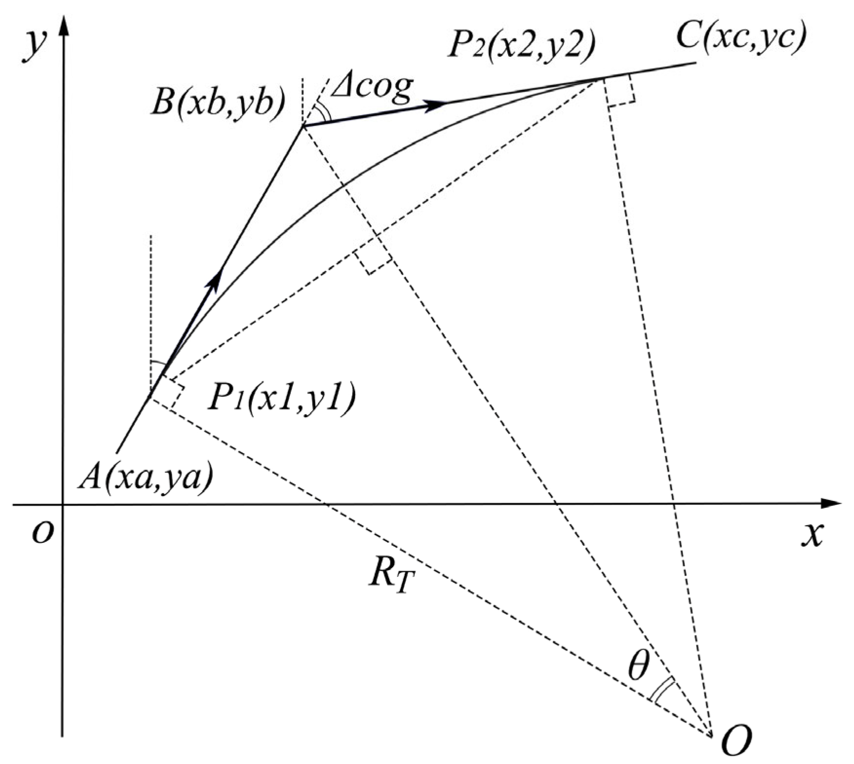
In
Figure 3 below, a certain path
is taken as an example. The coordinates of the three nodes are
,
, and
, and the coordinates of the two tangent points are
and
, respectively. According to the geometric relationship, the size of the center angle corresponding to the excessive arc is equal to the size of the ship’s course change angle
.
can be calculated according to the relationship between the ship’s course angle before and after turning. The calculation method of the ship course angle
(unit:
) is shown in Equation (2), where
denotes the course angle corresponding to vector
,
denotes the course angle corresponding to vector
, and the calculation method of
is shown in Equation (3).
where, when
, to avoid a denominator of zero,
.
The calculation method of the center half angle
corresponding to the arc is shown in Equation (4).
The distance between the starting point
of the arc and the inflection point
is calculated according to the trigonometric function relationship, as shown in Equation (5).
The coordinates of the starting point
P1 of the circular arc can be obtained by the proportionate relationship of the segment lengths, as shown in Equation (6). Where,
represents the Euclidean distance between points
A and
B.
Similarly, the coordinates of endpoint of the arc can be obtained.
The number of circular arc intermediate nodes is determined according to the interpolation accuracy. Here, interpolating once every center angle of
is taken as an example, and the coordinates of the next interpolation node can be obtained through the
rotating of the previous interpolation node about the center of the arc circle. Therefore, the center coordinates need to be calculated first. The line segment
and
are regarded as vectors
and
, respectively, and the orientation of the circle center relative to
can be obtained from the property of the cross product of the vectors. The calculation method is shown in Equation (7).
where
is the vector product of vector
and vector
. When
, the center of the circle is to the left of the vector
. When
, the center of the circle is to the right of the vector
. When
, two vectors are collinear or at least one of them is the zero vector.
Then, from the starting point of the arc, the unit vector
of the vector
is rotated
around the starting point of the arc in the direction of the center of the circle, and the unit vector pointing to the center of the circle is obtained. Multiplied by the radius length, the coordinates of the center of the circle can be obtained. The specific calculation method is shown in Equation (8).
The starting point of the arc rotates
around the center of the circle to obtain the coordinates of the next interpolation point
, as shown in Equation (9).
where
is the vector from the center of the circle to the start of the arc.
2.5. Local Path Detection and Correction Method of the Target Ship
According to the general idea of local path planning of the target ship proposed above, the next step is to realize the detection and correction of the target ship’s path according to the requirements of COLREGS and the effect of static obstacles on its navigation.
2.5.1. Logical Flow of Local Path Detection and Correction of the TS
According to the target ship’s path planning approach, when the distance between the TS and an interfering ship is within the specified safety distance at a given time, the target ship’s encounter situation should be analyzed and the navigability of the current path segment should be assessed. Based on the condition of the two ships’ collision risk [
37], encounter situation, and COLREGS requirements, the potential course interval of the target ship is preliminarily determined. Additionally, taking into account the influence of static obstacles and the relative position of the TS’s local target point, the course interval is further narrowed down. If the target ship is currently in a multi-ship encounter situation, it is necessary to further compress the course interval of the target ship by combining the complex encounter situation expression and prediction [
38] results based on bounded rational game. If the original path falls within this narrowed course range, no immediate course correction for the target ship is needed. Otherwise, a correction is required. The detailed logical flow is depicted in
Figure 4.
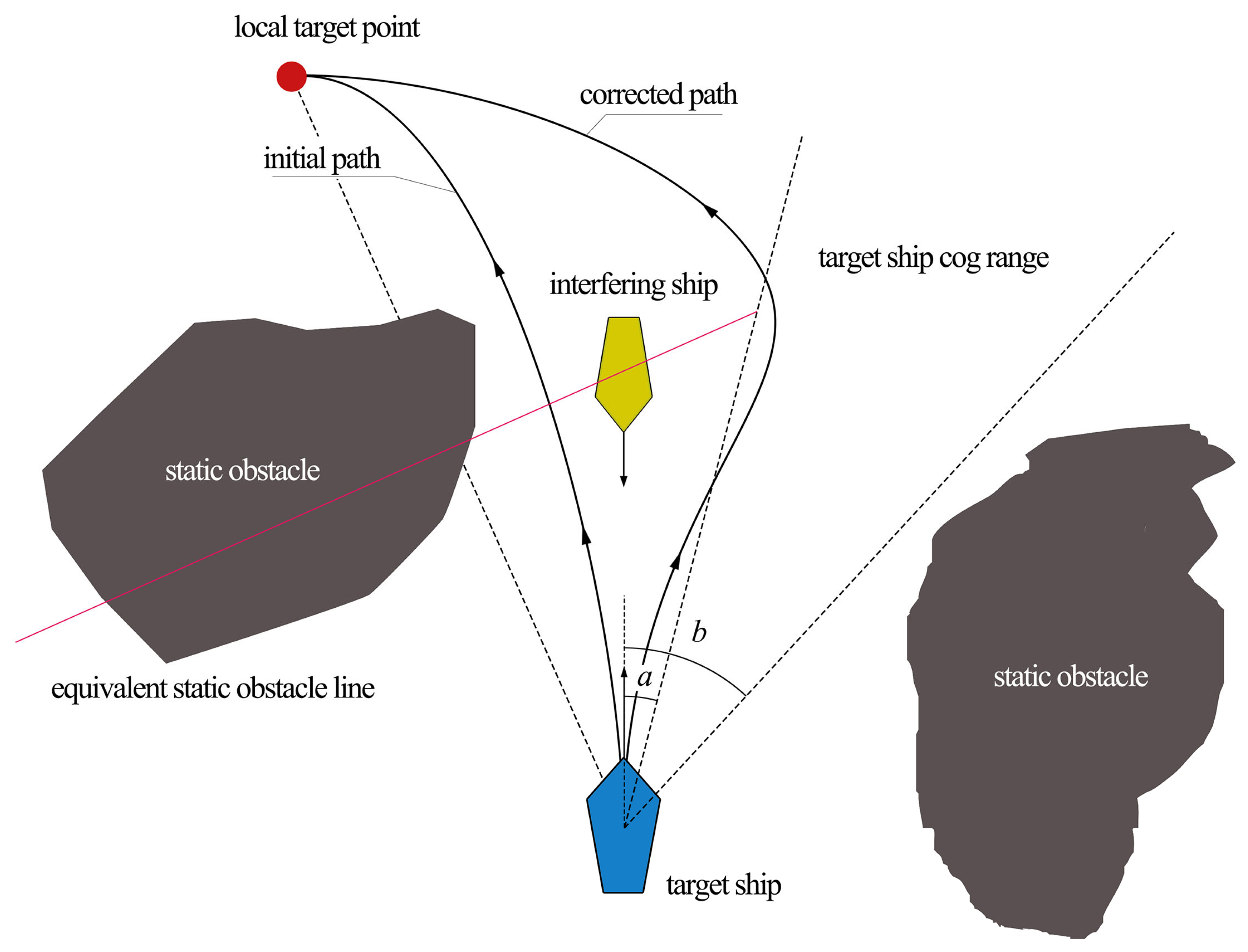
Based on the aforementioned logical flow, if the current path segment of the target ship is deemed unnavigable, it needs to be corrected. To achieve this, a method that generates time–space overlapping equivalent static obstacle lines based on situation inference is proposed. Essentially, the obstructive impact of interfering ships and static obstacles on the target ship’s navigation can be represented as one or more line segments within the scenario at the path planning moment. For instance, considering the logical flow in
Figure 4, the suitable target ship course interval
was determined. At this stage, the generation method for equivalent static obstacle lines for the TS is illustrated in
Figure 5, taking the two-ship encounter situation as an example. As presented in
Figure 5, the initial path of the target ship does not adhere to the avoidance responsibilities and obligations described in COLREGS for encounter situations. Sailing along this original path would increase the risk of collision or even result in accidents. However, by representing the influence of interfering ships and static obstacles as equivalent static obstacle lines, the planned path will not only effectively help avoid obstacles, but also ensure that the target ship’s navigation strategies comply with COLREGS. The process of determining navigability and correcting the target ship’s path segment is repeated continuously during the situation inference of the target ship until the entire path is deemed navigable, thus completing the target ship’s path correction.
In
Figure 5, the red line segment is an equivalent static obstacle line, which consists of a line segment perpendicular to the line between the TS and the local target point, and passes through the position of the interfering ship. In this line segment, the part contained in the course interval of the target ship is deleted. The logical flow chart of the equivalent static obstacle line’s construction method is shown in
Figure 6. In multiple-ship encounter situations, the form of the equivalent static obstacle line is similar to that of a two-ship encounter. The difference lies in the calculation of the target ship’s course interval, which is derived from the expression and prediction methods of complex encounter situations. Moreover, the equivalent static obstacle line intersects with the interfering ship which poses the highest collision risk with the TS. Therefore, the construction method is essentially the same.
2.5.2. Smooth Processing of the Target Ship’s Local Path
For the smooth processing of the target ship’s local path, in addition to adopting the method used for the interfering ship in
Section 2.4, the local path is divided into two parts to ensure that the sailing direction at the path’s start point is consistent with the current course of the target ship. The first part is from the current position of the target ship to position
, which is
distance forward along the target ship’s current course. The second part is from
to the final position of the target ship’s local path. The first part ensures that the initial segment of the planned path can conform to the ship’s movement law. Finally, the method described in
Section 2.4 is adopted to smooth the entire path.
3. Results
To verify the effectiveness and reliability of the local path planning method proposed in this study, it is compared with many common path planning methods, and the effectiveness of the method is verified by comparing and analyzing the characteristics of the path. The reliability is verified by the comparative analysis of the navigation conditions of ships along different local paths. In view of the high cost and risk of scenario construction of multi-ship encounter experiments, the simulation experimental method is temporarily adopted.
The basic idea of this experiment is mainly as follows. The proposed method is verified mainly from two perspectives. On the one hand, it is assumed that all interfering ships in encounter scenarios utilize the A* algorithm for path planning. The target ship, upon learning about the interfering ships’ paths, adopts different methods to plan its path, avoiding dynamic and static obstacles. A comparative analysis of the planned paths obtained using different methods is conducted to highlight the advantages of the proposed method. On the other hand, to simulate real navigation scenarios more realistically, the target ship, may not know the exact paths of the interfering ships. In this situation, the target ship utilizes the proposed method to plan its local path based on predictions of the interfering ships’ paths (assuming they all utilize the A* algorithm). The interfering ships, on the other hand, randomly select commonly used path planning algorithms to plan their paths. The adaptability of the target ship’s path to uncertain scenarios is analyzed to verify the advantages of the proposed method. To enhance the reliability of the experimental results, multiple random scenarios are set up for each group of experiments.
3.1. Experimental Setting
3.1.1. Experimental Ship and Parameter Setting
In this paper, the following method is adopted to construct a multi-ship encounter scenario involving dynamic and static obstacles: one target ship and four interfering ships are designated, with the interfering ships being randomly positioned within a radius around the target ship. Constraints are applied to ensure that the interfering ships generate in areas that significantly impact the target ship’s navigation. The course setting of the interfering ships is also controlled to form specific encounter situations with the target ship.
The parameters of the TS and ISs are outlined in
Table 2. Static obstacles are randomly generated as irregular polygons located farther than
distances from all ships. To facilitate the result presentation, the experiment duration is set to
min. The local target point of each ship is a coordinate point which is located in the place the target ship will reach in 120 min if the target ship is sailing straight according to its initial position, course, and speed, and it will remain unchanged throughout the simulation.
The in the table is set for relevant parameters of the interfering ships, which means that the length, width, and speed of the interfering ships fluctuate randomly based on the set value, and the fluctuation range is within . In this way, ships of different sizes and speeds in the scene are simulated, and the uncertainty of the real encounter scene is simulated as much as possible.
3.1.2. Experimental Procedure Setting
To verify the effectiveness of the local path planning method proposed in this paper, the paths obtained by using the proposed method for target ships are compared with those obtained by only using A* (A-Star), Dijkstra, RRT, PRM (Probabilistic Roadmap), PSO, and GA (Genetic Algorithm) algorithm. Four random scenarios are set. According to the basic idea of the control variable method, the A* algorithm is adopted for the path planning of interfering ships. The specific setting is shown in
Table 3. Through the consistency analysis of the local path planned by this method with the expected effect and the characteristics comparison analysis of the path planned by other methods, the effectiveness of the proposed method is verified. In the table,
represents the local path planning method proposed herein,
represents the target ship, and
represents interfering ships.
To verify the reliability of the proposed method, simulation experiments were conducted according to the scenarios set in
Table 3. In other words, both the target ship and the interfering ships sail according to their own planned paths, and the reliability of the proposed method is verified by comparing several indicators that can present the sailing efficiency and safety of the ship during the voyage.
In addition, in actual sailing scenarios, due to privacy, trade secrets, poor communication, and other reasons, the local paths or the path planning methods that interfering ships adopted are often not directly available. To enhance the realism of the simulation, the path planning methods for interfering ships are randomly assigned. Specifically, the interfering ships randomly select the A*, Dijkstra, RRT, PRM, PSO, or GA path planning algorithms. The target ship adopts the local path planning method proposed. During the target ship’s path planning, it remains unaware of the specific path planning method chosen by the interfering ships. As a provisional assumption, the interfering ships will utilize the A* algorithm for path planning and simulation, resulting in the collection of corresponding navigation indicators for the four scenarios mentioned above. Comparative analysis is conducted to further verify the proposed method’s reliability. To further increase the reliability of the experimental results, six repeated experiments were conducted in each scenario, and the specific scheme settings are shown in
Table 4. In the table, “Random” indicates that the interfering ships randomly select one of the six commonly used path planning algorithms mentioned above.
3.2. Experimental Data Processing
The experimental result data included the relevant parameters of all ships (including target ships and interfering ships). Part of the data is extracted and calculated [
39] to obtain the data required for the result analysis, which mainly includes the following:
Time series of the distance percentage between the TS and its local target point to its original distance (), which can present the navigation efficiency to a certain extent.
Time series of the minimum distance between the TS and ISs (), which can present the safety of ship navigation to a certain extent.
Time percentage of collision risk with value 1 for each ship (), which can also present the safety of ship navigation to a certain extent.
Taking scheme
as an example, the original data recording format of experimental results are shown in
Table 5. Due to the large amount of data, only specific time points,
,
, and
, were taken as examples. The table consists of attribute parameters of all ships in the simulation scenario that do not vary with time (first 6 rows, including the title row), followed by the state parameters of all ships at different times. In the experiment, a set of state parameters for all ships was generated every
s, as the situation inference duration was set to
s. In the actual recording of experimental results, the relevant parameters and state data of the same ship were recorded sequentially in the same row. To facilitate the presentation in the paper, we made some adjustments to the order of the data.
is calculated based on the parameters of the ship. The calculation method is depicted in Equation (10), where
indicates the distance between two points;
represents the ship’s current coordinate;
represents the coordinate of the ship’s local target point;
indicates the start coordinate value for calculation of the local target point.
can be obtained directly by comparing experimental data.
is obtained by counting the number of times each ship has a collision risk of 1 during the entire simulation period and then calculating its ratio to total times.
3.3. Experimental Process and Result Presentation
3.3.1. Experimental Process
In scenario
, according to the experimental scheme, the path planning results are shown in
Figure 7. The long white triangle with an arrow in the figure represents the TS, the long yellow triangle with an arrow represents the interfering ship, and the yellow filled area on the interfering ship represents the ship domain of the interfering ship. To present the ship identification in the figure as much as possible, and to maintain certain coordination between the size of the ship and the scene, the display size of the ship in the figure has been uniformly set to
times its actual size. The color of the target ship’s planned path is yellow, and that of the interfering ship’s planned path is green. To facilitate the distinction between the TS and ISs on the simulation interface, the TS’s initial course is set to 0 degrees, which corresponds to the upward direction on the simulation interface. The subgraph
shows the grid division and equivalent static obstacle lines of the target ship when the path planning method proposed in this paper is adopted. The red grid is the grid occupied by equivalent static obstacle lines.
In scenarios SCENE2, SCENE3, and SCENE4, the path planning results are shown in
Figure 8,
Figure 9, and
Figure 10, respectively, according to the experimental scheme.
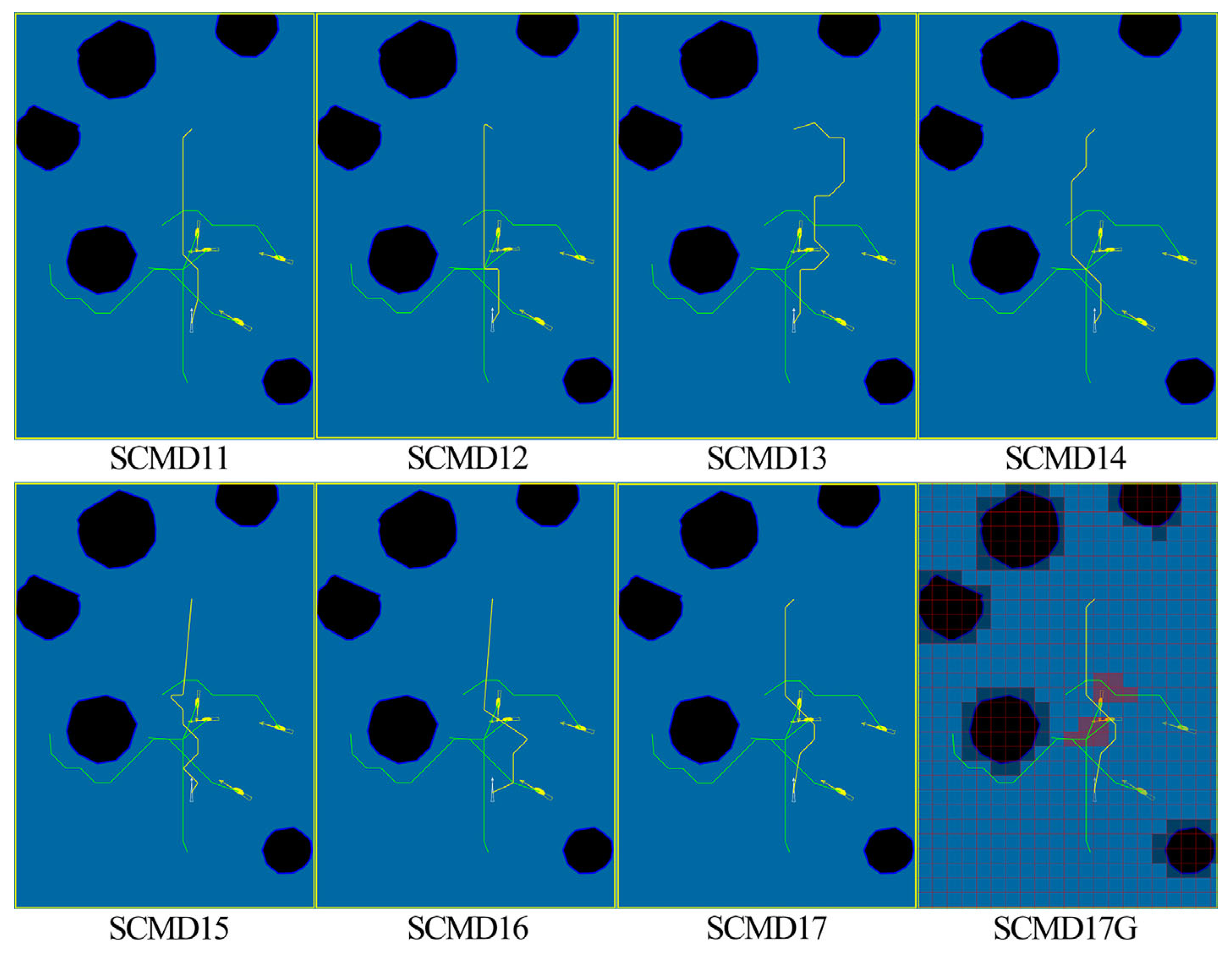
In the four scenarios, according to the experimental scheme, when the interfering ships randomly selected the path planning method, six repeated experiments were carried out. Taking the first experiment (
) as an example, the results were shown in
Figure 11. The path planning method proposed is adopted for target ships, and the effect of grid division and equivalent static obstacle line is consistent with the scheme
in the corresponding scenario (
represents the scheme using the path planning method proposed in this paper, such as
,
, etc.). Therefore, grid division and equivalent static obstacle line renderings are no longer repeated.
3.3.2. Reliability Verification Results
The
curves of the results for scenarios
are shown in
Figure 12.
The
curves of the results for scenarios
are shown in
Figure 13.
Figure 14 shows the data distribution of
of the target ship for scenarios
.
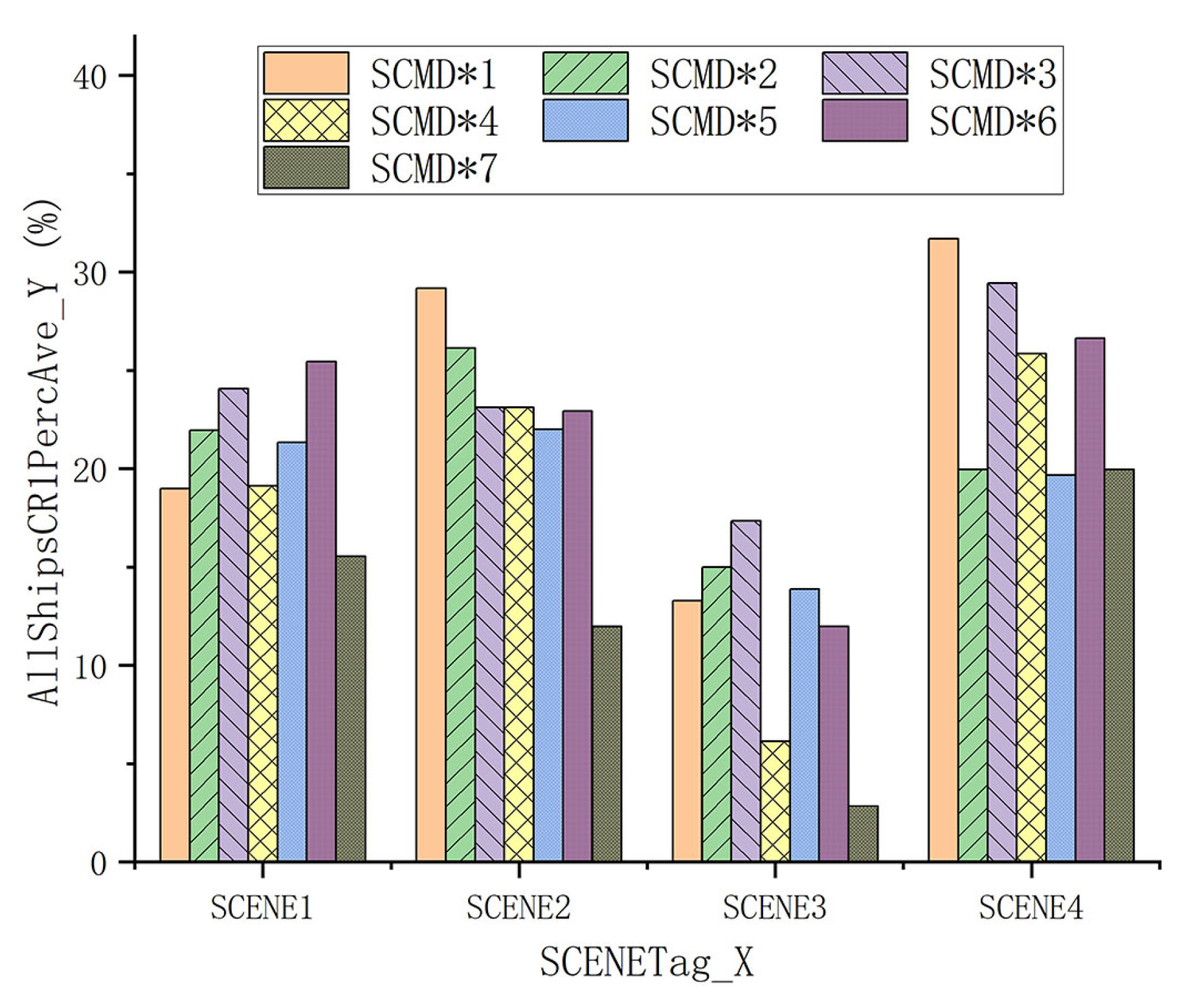
Figure 15 shows all ships’ mean value distribution of
for scenarios
.
3.3.3. Results of Six Rounds of Experiments under Uncertain Conditions
In the
rounds of experiments in different scenarios, the target ship adopted the proposed method in this paper; that is, the experimental scheme corresponding to
was selected. The
curves were consistent with the corresponding curves in
Figure 12, so they were not repeated. The
curves of the repeated experiments’ results are shown in
Figure 16.
In different scenarios, the data distribution of
of the target ship in six rounds of experiments with different scenarios are shown in
Figure 17.
In different scenarios, the mean value distribution of
data of all ships in
rounds of experiments with different scenarios are shown in
Figure 18.

 ,
, 


