
An Underwater Localization Method Based on Visual SLAM for the Near-Bottom Environment

1
School of Naval Architecture, Ocean and Civil Engineering, Shanghai Jiao Tong University, Shanghai 200240, China
2
State Key Laboratory of Ocean Engineering, Shanghai Jiao Tong University, Shanghai 200240, China
*
Author to whom correspondence should be addressed.
J. Mar. Sci. Eng. 2024, 12(5), 716; https://0-doi-org.brum.beds.ac.uk/10.3390/jmse12050716
Submission received: 20 March 2024
/
Revised: 23 April 2024
/
Accepted: 25 April 2024
/
Published: 26 April 2024
(This article belongs to the Topic Applications and Development of Underwater Robotics and Underwater Vision Technology)
Abstract
:The feature matching of the near-bottom visual SLAM is influenced by underwater raised sediments, resulting in tracking loss. In this paper, the novel visual SLAM system is proposed in the underwater raised sediments environment. The underwater images are firstly classified based on the color recognition method by adding the weights of pixel location to reduce the interference of similar colors on the seabed. The improved adaptive median filter method is proposed to filter the classified images by using the mean value of the filter window border as the discriminant condition to retain the original features of the image. The filtered images are finally processed by the tracking module to obtain the trajectory of underwater vehicles and the seafloor maps. The datasets of seamount areas captured in the western Pacific Ocean are processed by the improved visual SLAM system. The keyframes, mapping points, and feature point matching pairs extracted from the improved visual SLAM system are improved by 5.2%, 11.2%, and 4.5% compared with that of the ORB-SLAM3 system, respectively. The improved visual SLAM system has the advantage of robustness to dynamic disturbances, which is of practical application in underwater vehicles operated in near-bottom areas such as seamounts and nodules.
1. Introduction
Underwater inspection and surveys are important underwater applications such as seafloor resource exploration. Visual technology is widely used for Underwater inspection and surveys. Deep-sea mining and seafloor oil and gas exploration utilized by AUVs are popular topics to research [1,2,3]. Wang uses a robust Real-Time AUV Self-Localization method for deep-sea exploration [4]. Hong presents a portable autonomous underwater vehicle (AUV) named Shark for vision-based underwater inspection [5]. Chemisky conducts a review of the close-range optical methods for the underwater oil and gas industry [6]. Stenius presents the application of AUVs for seaweed farm inspection [7]. Underwater visual localization technology such as underwater visual SLAM is one of the key technologies for underwater inspection tasks. Underwater visual SLAM is utilized for the trajectory localization of underwater vehicles and the construction of the surrounding environment by feature matching and tracking the captured video images in the underwater scene [8,9]. Underwater navigation is necessary for the operation of autonomous underwater vehicles [10]. The position of the underwater vehicle is a prerequisite for underwater navigation [11]. Due to the absence of GPS information in the underwater environment, underwater localization is difficult and has been extensively investigated. Multi-sensor information fusion is commonly applied to obtain the position information of autonomous underwater vehicles. A passive inverted Ultra-Short Baseline (piUSBL) positioning system is proposed by Wang [12], which provides accurate and instantaneous positioning for small Autonomous Underwater Vehicles (AUVs) by single-beacon tracking at low cost and power consumption. The acoustic image processing based on multi-beam bathymetric sonar data is utilized in underwater terrain-aided navigation, which is more stable when direction error is more significant than 10°, and the accuracy is approximately 50% better. At the same time, noise and scale vary in the real-time images compared with the terrain contour matching algorithm [13]. In addition to using additional sensor information to aid navigation, improved underwater navigation algorithms are also proposed for underwater localization [14,15,16]. However, accumulated errors are unavoidable in traditional integrated navigation methods, and devices such as DVL and USBL fail in near-bottom environments. Machine vision can work steadily for long periods with tiny cumulative time errors [17,18]. Thus, underwater visual SLAM has been developed and applied for location awareness of the underwater environment and assisted navigation in recent years, which has excellent potential for unmanned surveys and free cruising applications [19,20,21,22,23]. The application of underwater SLAM is widely studied. Issartel uses SLAM technology for the underwater military to achieve underwater hiding for tasks [24]. Zhang utilizes BSLAM (Bathymetric Particle Filter SLAM) which is accurate and fast for oceanographic surveys, demining, and seabed mappings [25]. Yang proposes a SLAM localization algorithm using forward-looking sonar for deep-sea mining [26]. Mahajan proposed a pilot aid using visual SLAM for seabed surveying applications [27].
Joshi verifies and analyzes multiple visual algorithms in the underwater environment, such as OKVIS, SVO, ROVIO, VINS-Mono, and ORB-SLAM3, based on the datasets tested [28]. The Fugu-f (Fugu flexible) system is presented to provide visual localization in submarine tasks such as navigation, surveying, and mapping under good visibility with the main advantages of robustness and flexibility [29]. An omnidirectional and positioning-tolerant miniaturized prototype AUV docking system based on the integrated visual navigation and docking algorithm is proposed to solve the planar-type docking issues in a transparent water environment [30]. Although underwater visual SLAM has been used for AUV navigation tasks, it is not always feasible for all cases due to limitations in underwater image quality. A keyframe-based monocular visual odometry method is proposed by adding a re-tracking mechanism to enhance optical flow tracking, realizing a robust vision-based underwater localization in the turbid underwater environment [31]. However, underwater raised sediments sometimes occur in near-bottom environments. The feature matching of visual SLAM is affected by the randomness of motion direction of the underwater raised sediments. There are few studies on this influence.
When visual SLAM is affected by the external environment, there are two main solutions: adding sensors or image pre-processing [32]. Since the role of visual SLAM is auxiliary rather than central in underwater navigation, the solution of adding sensors for visual SLAM is not adopted in underwater navigation. Image pre-processing for visual SLAM includes two parts: image classification and image denoising.
Because the raised sediment phenomenon is occasional and does not always exist, image classification can reduce the computational effort to increase real-time performance, which is essential for visual SLAM. Image classification methods use underwater image features such as color, texture, shape, and spatial distribution to classify images. Mittal uses deep learning and image color analysis to classify underwater photographs and recognize numerous things, such as fish, plankton, coral reefs, submarines, and the gestures of sea divers [33]. Mahmood proposes a new image feature (called ResFeats) extracted from images’ textures and shapes. ResFeats has state-of-the-art classification accuracies on MLC, Benthoz15, EILAT, and RSMAS datasets compared with the traditional CNN method [34]. Lopez-Vazquez designs a pipeline using integrated spatial distribution and temporal dynamics information to perform well in mobile and sessile megafauna recognition and classification tasks [35]. The accuracy value of the classification method reaches 76.18% in deep-sea videos taken at 260 m depth in the Barents Sea. As the underwater raised sediments have the characteristics of noticeable color difference with seawater and strong randomness of shape and spatial distribution, the color features of the underwater image are utilized for image classification. However, the color of the underwater raised sediments is similar to that of the sea floor in the near-bottom environment, affecting image classification. There are few studies for image classification based on image color features in near-bottom environments.
The images that need to be denoised are obtained through image classification. The image-denoising methods include learning-based and filtering-based [36]. Deep learning techniques such as convolutional neural networks (CNN) are widely utilized for the image-denoising method of learning [37]. Pang proposed a data augmentation technique called corrupted-to-corrupted (R2R) to achieve unsupervised image denoising. The method is competitive to representative supervised image denoising [38]. Li proposes a self-supervised image denoising (SSID) method for real-world sRGB images to seek spatially adaptive supervision on real-world sRGB photographs [39]. Dasari uses GAN architecture and histogram equalization to enhance the underwater images. The 2186 real-world underwater images are used for verification [40]. Raj uses SURF (Speeded-Up Robust Features) and SVM (Support Vector Machines) algorithms to attain maximum accuracy in underwater image classification [41]. Moghimi uses a two-step image enhancement method which includes color correction and a convolutional neural network (CNN) with deep learning capability to realize the underwater image quality enhancement [42].
However, underwater raised sediments are often random and unknown during underwater operations. The background has also changed due to the movement of underwater vehicles. There are not enough sample sets to train and learn underwater image classification and denoising in an underwater survey task when the operating area is unknown. Terrestrial training models are directly used whose results are not good. Therefore, filtering-based methods are utilized for image denoising. There are extensive studies on filtering-based image-denoising methods [43]. Kumar proposes different median filter methods to eliminate salt-and-pepper noise [44]. Sagar presents a circular adaptive median filter (CAMF) to denoise salt-and-pepper noise of varying noise densities for magnetic resonance imaging (MRI) images [45]. It can be seen that the primary filter-based methods are effective for salt-and-pepper noise. The underwater raised sediments are similar to salt-and-pepper noise in terms of significant color differences. However, there is a big difference in size and shape. There is little research on underwater raised sediments denoised through filter-based methods.
In this paper, an improved visual SLAM system is proposed to reduce the impact of the underwater raised sediments to the feature matching of the visual SLAM to improve the robustness of the visual SLAM. The weights of pixel position are added to improve the color recognition method in HSV color space for image classification to reduce the interference of similar colors on the seabed to improve the real-time of the visual SLAM. An improved adaptive median filtering method is proposed by utilizing the mean value of the window border pixels as a filtering criterion, which enhances the retained feature information of the classified images to retain more original features of the images to improve the success rate of feature matching. The filtered images are finally processed by the tracking module to obtain the trajectory of underwater vehicles and the seafloor maps. The video datasets captured in the western Pacific Ocean at 3000 m depth are processed by the improved visual SLAM system. Keyframes, mapping points, and feature point matching pairs are extracted from the improved visual SLAM system, which improved by 5.2%, 11.2%, and 4.5%, respectively. The improved visual SLAM system has the advantage of robustness to dynamic disturbances such as underwater raised sediments, water bubbles, etc., which is of practical application in underwater vehicles operated in near-bottom areas such as seamounts, rockfall, and nodules.
This paper is organized as follows. Section 2 describes the underwater raised sediments phenomenon and proposes a novel visual SLAM system in the underwater raised sediments environment. Section 3 presents the image classification and denoising methods to achieve image pre-processing. Then, image classification and quality evaluation results are obtained to verify the effectiveness of the methods. Section 4 shows the experimental tests and results. Section 5 presents the conclusions of the paper.
2. The Visual SLAM System for Underwater Raised Sediments Environment Establishment
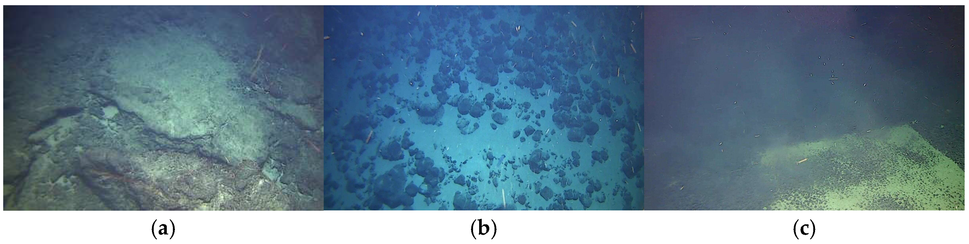
Underwater images taken by the autonomous underwater vehicles while working at a depth of 3000 m in the western Pacific seamount area are shown in Figure 1. Underwater no-raised sediment images that expressed different areas during the movement and operation of autonomous underwater vehicles are shown in Figure 1, respectively. The seamount area is shown in Figure 1a, the rockfall area is shown in Figure 1b, and the nodules area is shown in Figure 1c. The images of the underwater different areas are clear and rich in texture detail. When the autonomous underwater vehicles operate in the seamount area near the bottom, the localization of the low-cost autonomous underwater vehicles is realized generally by an inertial navigation system (INS) with IMU as the core sensor and integrated navigation assisted by underwater acoustic equipment such as Doppler velocity log(DVL) and ultra-short baseline (USBL). However, there is a dead band due to the installation position of the Doppler velocity log(DVL) on the low-cost autonomous underwater vehicles that are too close to the seabed. The ultra-short baseline (USBL) is disturbed by bubbles generated by propeller disturbance. Underwater acoustic equipment fails when it moves and inspects underwater near-bottom seamount areas. Because the images taken in the underwater seamount area are clear and texture features are sufficient, the visual localization method is utilized instead of underwater acoustic equipment to assist integrated navigation.
Due to the movement of the underwater vehicle and the disturbance of the propeller near the bottom, the underwater raised sediments will sometimes be generated in near-bottom areas in Figure 2. The degrees of the underwater raised sediments are different in different areas. The underwater raised sediment in the seamount area is light degree shown in Figure 2a, the underwater raised sediment occupies a small part of the images, and most of the feature information of the underwater images is retained compared with the origin images; the underwater raised sediment in the rockfall area is medium degree shown in Figure 2b, the underwater raised sediment takes up most of the images, and most of the feature information of the underwater images are influenced by the underwater raised sediments; and the underwater raised sediment in the area of the nodule is heavy degree shown in Figure 2c, and there is fog dust apart from line dust. Few of the feature information is retained in underwater images. The impact of underwater raised sediments on visual localization techniques such as ORB-SLAM3 is mainly divided into two parts: the original images are obscured by the underwater raised sediments, reducing the feature information. Image recovery techniques are generally used to recover characteristics, but image recovery techniques require accurate image information, which is often unknown in the underwater near-bottom environment; the direction of motion of underwater raised sediments is random and different from the motion direction of underwater vehicles. When the degree of underwater dust increases, it will cause a reduction in the number of feature point-matching pairs due to the directional consistency detection of the tracking module. Therefore, image pre-processing is necessary to remove raised sediments which can increase feature point matching pairs and increase the robustness of visual SLAM.
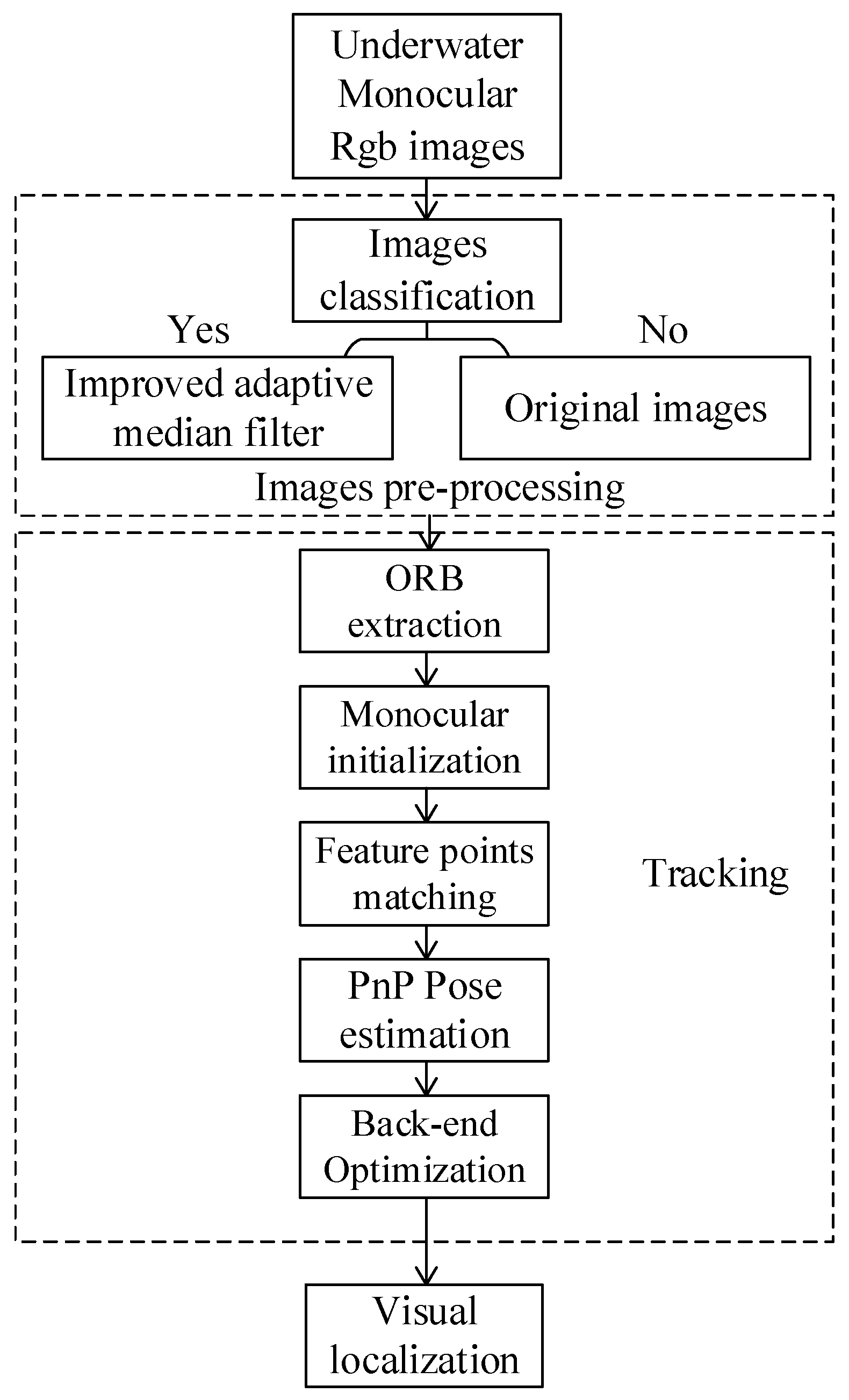
An improved visual SLAM system is proposed for visual localization in the underwater raised sediments environment. The block diagram of the improved underwater visual SLAM system is shown in Figure 3. The monocular video is extracted frame by frame into an image stream, and each image is classified as to whether or not it has to be pre-processed. The improved adaptive median filtering algorithm is then utilized to perform image denoising on the raised sediment images. The ORB feature points are retrieved from pre-processed images, and the matching between the initial frame and the current frame is achieved by performing monocular initialization using the Homography matrix or the Fundamental matrix. The pose of the initialization is obtained by Epipolar Geometry. The matching feature point pairs are then projected into 3D map points using triangulate. Via tracking the motion model or key frame, feature matching is conducted. Then, the pose of the current frame is estimated by PnP (Perspective-n-Point) such as DLT (Direct Linear Transform), and optimized by the Back-end Optimization such as BA (Bundle Adjustment). The Loop Closure Detection is not necessary, as the underwater vehicle does not return to its starting point in the underwater exploration task.
3. Underwater Raised Sediments Image Pre-Processing Method
The underwater raised sediments image pre-processing method consists of image classification and image denoising, which removes dynamic interference in underwater images. The proposed image classification method is presented in Section 3.1. The underwater images are classified based on the color recognition method in HSV color space to obtain the images that need to be denoised by adding the weights of pixel location to reduce the interference of similar colors on the seabed. The improved adaptive median filtering method is proposed in Section 3.2. The improved adaptive median filter method is proposed to denoise the classified images by using the mean value of the filter window border as the discriminant condition to reduce the disturbance of underwater raised sediments and to retain the original features of the image. The filtered image quality assessment is shown in Section 3.3 through Mean Gradient (MG), Structural Similarity (SSIM), and Peak Signal-to-Noise Ratio (PSNR) methods.
3.1. The Proposed Image Classification Method
The flowchart of the proposed image classification method is shown in Figure 4, where the dotted box indicates the proposed image classification method. The original underwater images are first converted to HSV color space. The location weight values are set by the application scenes added in color recognition to reduce the interference of similar colors on the seabed. When the color recognition value of the image exceeds the discriminant threshold, the image needs to be filtered; otherwise, the original image is retained. The classified images are entered into the filter module, and the remaining images are entered directly into the tracking module.
The color space of an image includes RGB (Red, Green, and Blue) color space, CMY (Cyan, Magenta, and Yellow) color space, and HSV (Hue, Saturation, and Value) color space, etc. The CMY color space is used to represent a printed image and the digital images commonly use RGB color space and HSV color space. The RGB color space is the most used way to describe electronic images, but parameter changes in RGB can cause significant color changes. Therefore, it is not suitable for classifying images by color. Conversely, the HSV color space can be used to classify underwater images by setting a parameter range for the color.
Images are classified based on the color and location of the underwater raised sediments to determine if the images need to be denoised. The color of the underwater raised sediments is different from the water, so the image classification can be realized through color recognition. However, since the seabed’s color is similar to that of the underwater raised sediments, location is also necessary to determine the color weights. Depending on the camera mounting angle and distance from the bottom, underwater-raised sediments in near-bottom images suspended in seawater are present in the image’s upper half, not the seafloor’s lower half. Therefore, the yellow pixel weight for the seawater is , and the yellow pixel weight for the seabed is , , The size of the photo is , and the pixel point location is expressed by , and the location weight is expressed in Equation (1):
The images captured by the underwater camera are stored in RGB color space. RGB color space uses a linear combination of three-color components to represent color. But in color recognition, any color is highly correlated with these three components, so it is not intuitive to continuously change colors, and these three components need to change to adjust the color of the image. Therefore, we need to convert the RGB into HSV color space expressed in Equation (2). The color component value of a pixel point is R, G, B, respectively; is the maximum of the three color components, is the minimum of the three color components, is the luminance Value, is the Saturation, and is the hue. Color is only highly correlated with Hue. Adjusting Saturation and Value will result in similar colors.
The original purpose of image classification was to reduce the amount of computation. The purpose of the increase in position weights is to increase the accuracy of image classification based on color. The limitations of the positional weights are such that it is not able to correctly classify all images, but the ORB-SLAM3 system itself is robust to images that are not correctly classified. The range of values for the color of underwater raised sediments is set in Equation (3):
where H is expressed using radians.
is a Boolean value, if the HSV value of the pixel satisfies Equation (3), the value is 1; otherwise, it is 0. is the position weight, is the number of pixels identified by adding the position weight, and is the discriminant threshold.
When , the image is considered to need image noise denoising, otherwise the original image is kept.
For the underwater videos of the different areas, 2000 underwater images were extracted at 15 fps, respectively. Let discriminant threshold , there are classification results shown in Table 1, Table 2 and Table 3. The ‘real’ respects the true results which are used to compare. The title of Need-Denoising shows the number of classified images. The title of Original shows the number of the remaining images. Accuracy is obtained by the number of correctly detected images divided by the total number of images.
The image classification in the seamount area has high accuracy, when . The real number of Need-Denoising images in the rockfall area is more than that in the seamount area. The number of Need-Denoising images in the rockfall area is more than the real number because the underwater raised sediment takes up most of the images. During the underwater operation of an underwater vehicle, underwater raised sediments are not present at every moment, so not all the images need to be denoised. The image classification method proposed in this paper can significantly reduce the computational effort and retain original image features.
3.2. The Improved Adaptive Median Filtering Method
The flowchart of the improved adaptive median filtering method is shown in Figure 5, where the dotted box indicates the improved adaptive median filtering method. One pixel in the classified image is chosen, and the filter window length is initialized (set in 3). The mean value of the window border is compared with the mean value of the background, which is the mean value of the image. The window length is determined through the compared result based on the Pauta criterion. The mean value of the window border is utilized for the filter discriminant condition, which is compared with the value of the chosen pixel to decide whether to filter or not. The median value of the filter window is used to replace the filtered pixel. Otherwise, the original value is retained. Then, the next pixel repeats the same steps until the end of the loop. The filtered image is entered in the tracking module at last.
Underwater-raised sediments are small in the image, and the color is significantly different from seawater. Due to the relative motion of underwater raised sediments and underwater vehicles, there is a smear in the underwater image, as shown in Figure 2. The smear can be seen as a kind of line salt-and-pepper noise. Adaptive median filtering can effectively filter out salt-and-pepper noise of different sizes through adaptive window size. The original adaptive median filter is more suitable for granular noise. This paper proposes an improved adaptive median filter for line noise. The window size is determined according to the mean pixel value of the window border compared with the mean pixel value of the background. Then, the center point is compared with the mean pixel value of the window border to decide whether to filter or retain. If the filter is decided, the filtered pixel points are replaced by the median value within the window. The improved adaptive filtering has a better effect of denoising the line noise.
The underwater raised sediments are small in the image, and the color is significantly different from seawater. Due to the relative motion of underwater raised sediments and underwater vehicles, there is a smear in the underwater image, as shown in Figure 2. The smear can be seen as a kind of line salt-and-pepper noise. Adaptive median filtering can effectively filter out salt-and-pepper noise of different sizes through adaptive window size. The original adaptive median filter is more suitable for granular noise. This paper proposes an improved adaptive median filter for line noise. The window size is determined according to the mean pixel value of the window border compared with the mean pixel value of the background. Then, the center point is compared with the mean pixel value of the window border to decide whether to filter or retain. If the filter is decided, the filtered pixel points are replaced by the median value within the window. The improved adaptive filtering has a better effect of denoising the line noise.
- Filter window size determination
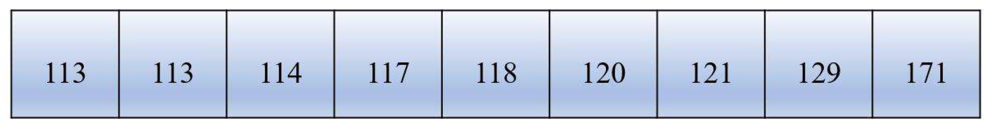
The size of the filter window should be chosen to be as small as possible to retain more feature information about the underwater images. Thus, an adaptive filter method for the selection of filter window size is applied. The window is a square, and the initial value of the window length is 3. The gray value of the center point is shown in the cell of the window, as shown in Figure 6. The gray value of the center point is 171, and the pixels are sorted from most minor to most significant, as shown in Figure 7. The maximum gray value of the window is 171, the maximum gray value of the window is 113, and the median gray value of the window is 118. The mean gray value of the window border is 139.5. The mean of the background grayscale value is , and the standard deviation of the background grayscale value is . According to the Pauta criterion, if , determine the window length and enter the filtering session. Otherwise, add 2 to the window length and perform a new cycle until the window length is determined. The maximum value of the window length is . When , the filtering session is entered directly.
- 2.
- Filtering session
The method of mean value filtering is a common method for image denoising. However, the method of median filtering has less computational effort which increases the real-time performance of ORB-SLAM3, and the image processed by median filtering retains more feature information compared to mean filtering to improve the stability of the ORB-SLAM3. Therefore, the method of median filtering is applied for the underwater image denoising. The gray value of the center point is , the mean gray value of the window border is in Figure 8, and the standard deviation of the background grayscale value is . According to the Pauta criterion, if , the gray value of the center point is replaced by the median gray value of the window , otherwise the original value is retained.
3.3. The Filtered Image Quality Assessment
The assessment of image quality focuses on three aspects. Firstly, measuring whether the sharpness and contrast of the images are effectively improved, is generally evaluated by the Mean Gradient (MG). Secondly, detecting whether the enhanced images retain the information of the original image as much as possible, which generally uses Structural Similarity (SSIM) and Peak Signal-to-Noise Ratio (PSNR) to calculate the structural similarity of the images. Finally, visually analyze the denoising effect by observing the images before and after processing.
- (1)
- Mean Gradient (MG) is used to measure the contrast of images, and the larger the mean gradient, the greater the contrast.
- (2)
- Structural Similarity (SSIM) is applied to evaluate the pixel correlation between the processed and original images.
- (3)
- Peak Signal-to-Noise Ratio (PSNR) reflects the degree of similarity between the processed and original images and is similar to the SSIM function.
MSE is the Mean Square Error (MSE) of the two images before and after processing and is the number of pixel bits in binary, which is taken as 8.
The assessment of image quality focuses on three aspects. Firstly, measuring whether the sharpness and contrast of the images are effectively improved, is generally evaluated by the Mean Gradient (MG). Secondly, detect whether the enhanced images retain the information of the original image as much as possible, which generally uses Structural Similarity (SSIM) and Peak Signal-to-Noise Ratio (PSNR) to calculate the structural similarity of the images. Finally, visually analyze the denoising effect by observing the images before and after processing.
Because the degree of underwater raised sediments is severe in the rockfall and nodules areas, the feature matching of ORB-SLAM3 is affected leading to initialization failure. The effectiveness of image pre-processing and the enhancement of ORB-SLAM3 is validated in the seamount area.
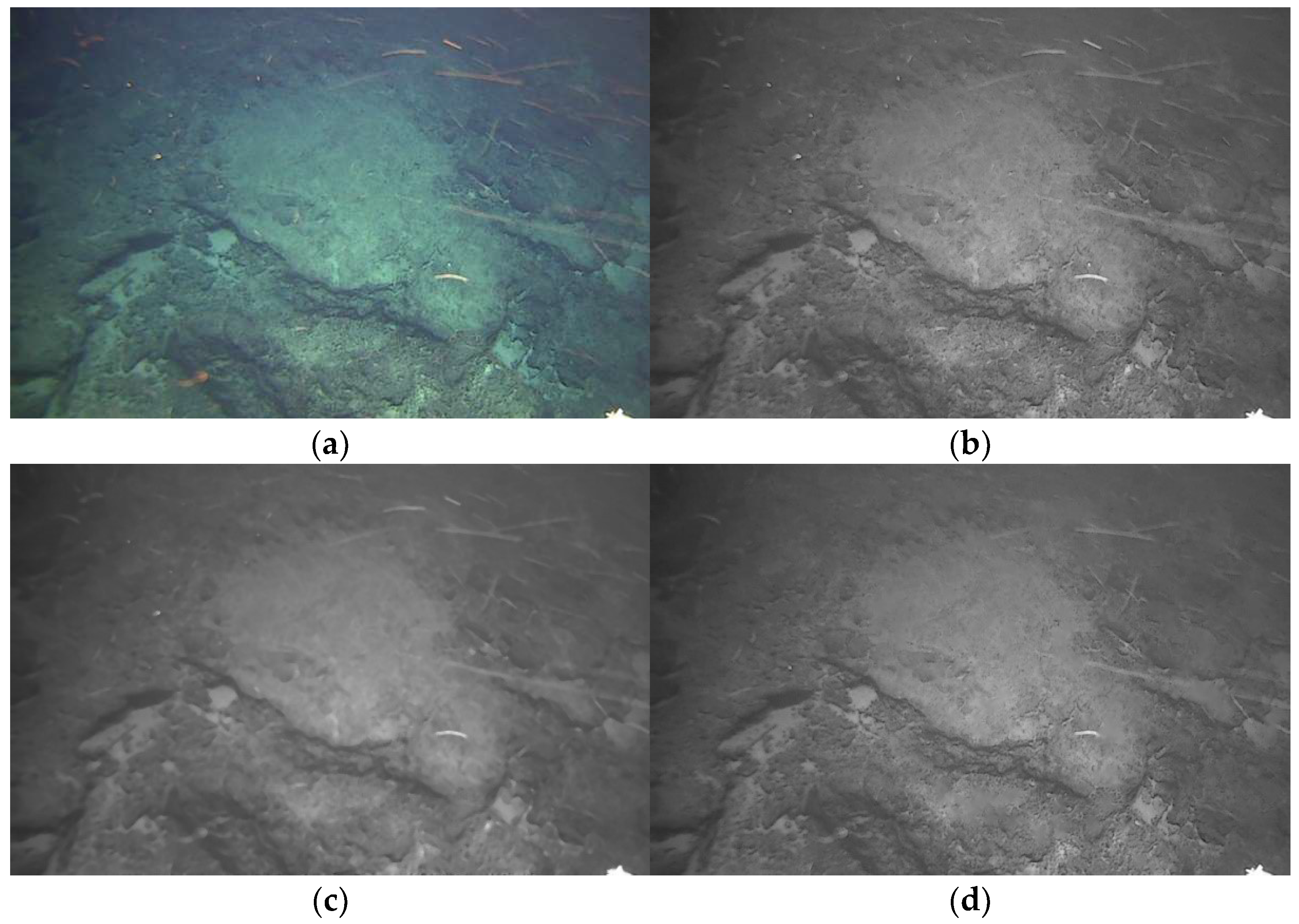
An original color image of underwater raised sediments is shown in Figure 9a, and its grayscale image is shown in Figure 9b. The results of the traditional adaptive median filter (TAMF) and improved adaptive median filter (IAMF) on the original grayscale image are shown in Figure 9c and Figure 9d, respectively. The image quality assessment results are shown in Table 4. The metrics are the three assessment methods. The TAMF and IAMF are the abbreviations of the two filter methods. The improvement is calculated by the difference value of the two filter methods divided by the value of the traditional adaptive median filter. The image contrast is significantly improved by 106.7%. Image similarity is improved by 4.6%, and image quality by 1.1%. More image similarity means more original information preserved, which can be seen by observing the images directly. The improved adaptive median filter has a better denoising effect on the line noise than the traditional adaptive median filter.
4. Experimental Verification and Analysis
The experimental environment is shown in Section 4.1. The experimental procedures and results are shown in Section 4.2. The datasets of seamount areas captured in the western Pacific Ocean are processed by the improved visual SLAM system. The initialization is recorded, which proves that the improved system is easy to succeed. The keyframes, mapping points, and feature point matching pairs extracted from the improved visual SLAM system are improved by 5.2%, 11.2%, and 4.5% compared with that of the ORB-SLAM3 system, respectively. The improved visual SLAM system has the advantage of robustness to dynamic disturbances such as underwater raised sediments, water bubbles, etc., which is of practical application in underwater vehicles operated in near-bottom areas such as seamounts, rockfall, and nodules.
4.1. The Experimental Environment for the Seamount Images
The experimental environment is shown in Table 5. ORB-SLAM3 is the popular visual SLAM method, which is selected for the comparison system. The SLAM operating system is Ubuntu 20.04, and the image-processing operating system is Windows 10. The image processing program software is MatLab R2022a, and the computer CPU is Ryzen7.
4.2. Experimental Procedures and Results for the Seamount Images
The experimental tests were conducted using the videos captured by ROV in the seamount area at a frame rate of 15 fps, with 2000 consecutive frames each to form image datasets. ORB-SLAM3 is the famous monocular vision SLAM system being used for comparison. The datasets are processed under proposed visual SLAM systems. The initialization phase, mapping, and trajectory are recorded. The number of keyframes, matched point pairs, and map points are extracted. The analysis was performed according to the experimental results.
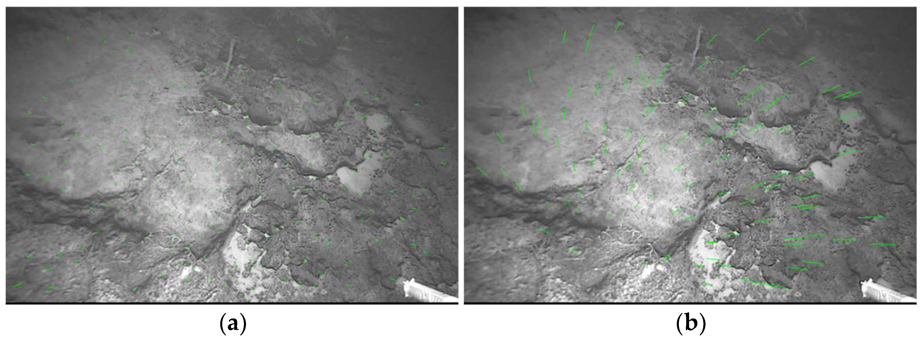
The initialization phase is recorded in Figure 10 and Figure 11. The tests are carried out several times, where Test 1 and Test 2 are the two representative tests. Initialization failure occurred in the initialization phase due to the influence of underwater raised sediments under the ORB-SLAM3 system in Figure 10. There are not enough feature points matched to finish the initialization in Figure 10. The feature of the seamount image is not richer than the terrestrial environment. Initialization failure occurs when other dynamic disturbances exist, such as water bubbles and underwater raised sediments. Initialization was rapidly successful due to image pre-processing for the underwater raised sediments under the proposed system in Figure 11. Initialization under the proposed system is easy to succeed in the underwater raised sediments environment.
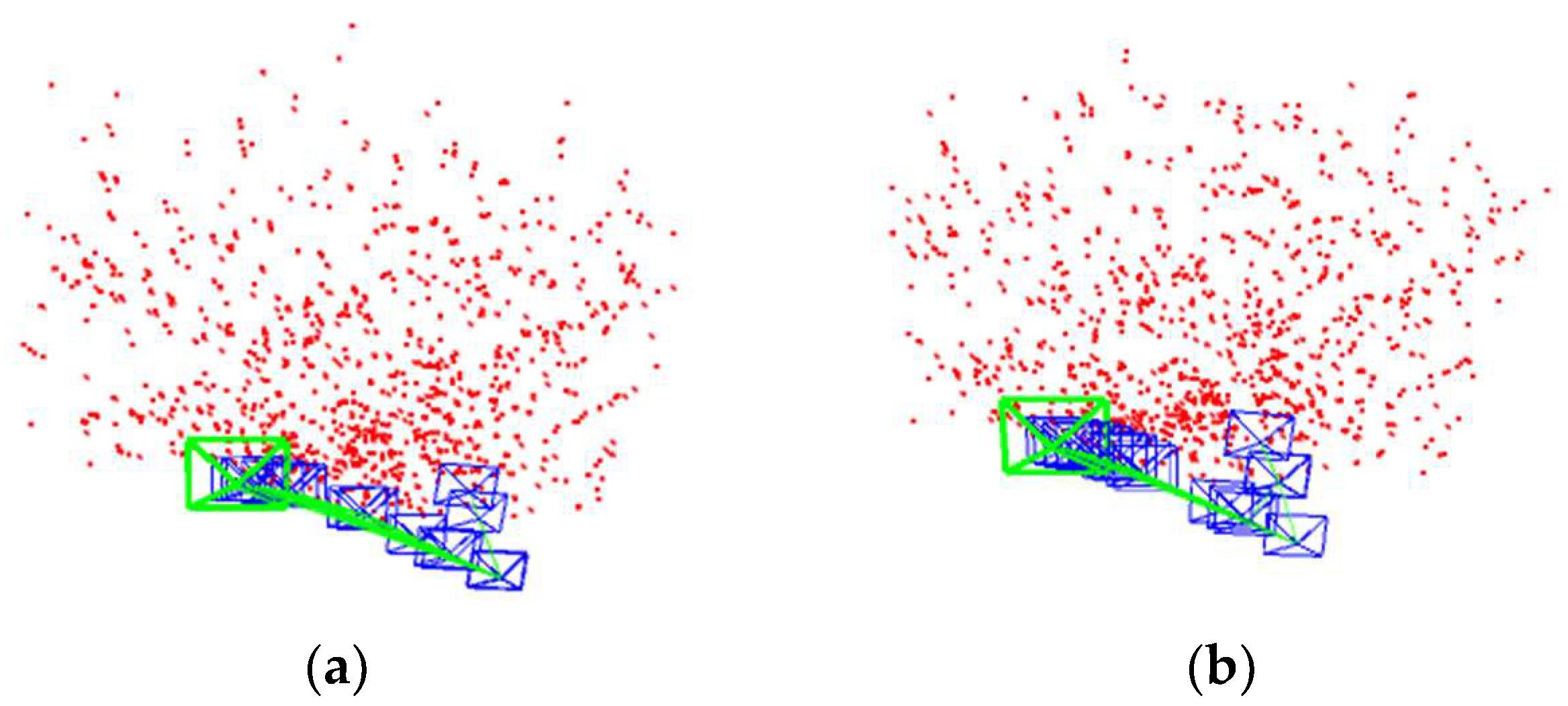
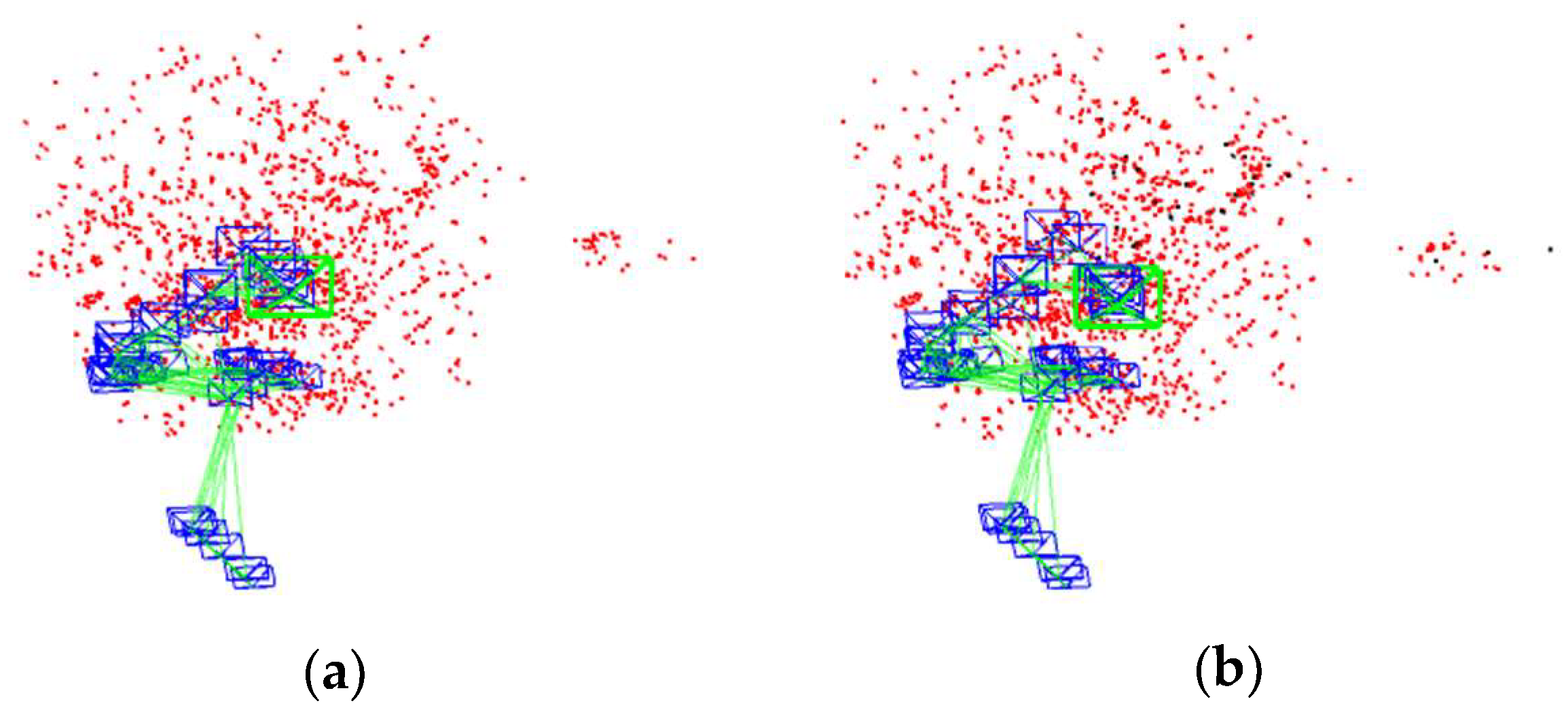
Mapping and trajectory in the initialization phase under the proposed system were recorded in Figure 12. Mapping and trajectory in the end phase under the ORB-SLAM3 system were recorded in Figure 13. Mapping and trajectory in the end phase under the proposed system were recorded in Figure 14. Different representative moments were recorded continuously such as moment 1 and moment 2 in Figure 12, Figure 13 and Figure 14. Mapping and trajectory under the proposed system are more obtained than the ORB-SLAM3 system, which can be seen from the number of keyframes and map points. The underwater raised sediment images in the datasets processed by the proposed system caused matching point pairs to increase. Increasing matched point pairs provides more accurate tracking, which is proved by more keyframes and mapping points obtained.
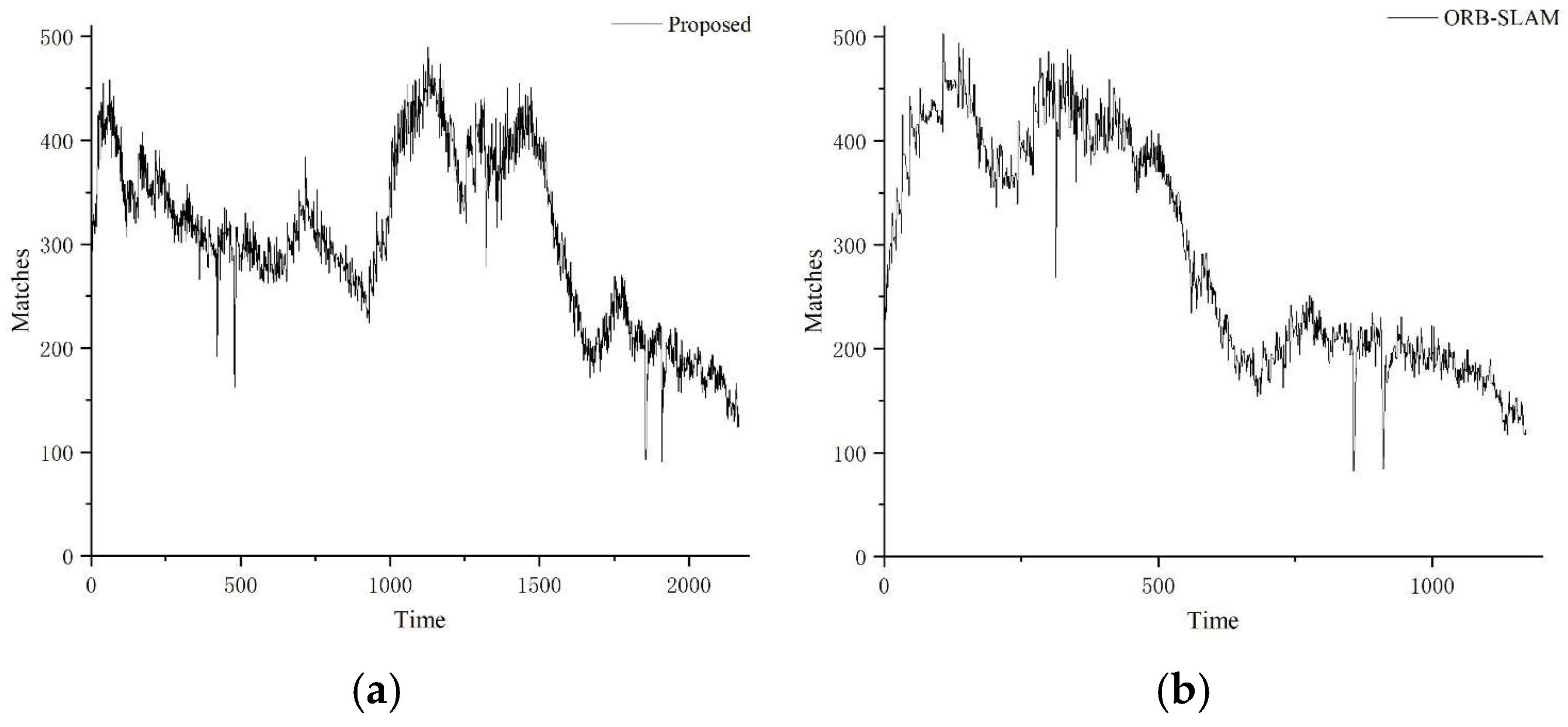
The number of match point pairs (Matches) under both systems is shown in Figure 15. The number of match point pairs of the proposed system is shown in Figure 15a; the number of match point pairs of the ORB-SLAM3 system is shown in Figure 15b. The statistical results of match point pairs are shown in Table 6. The title of Max is the maximum value of the match point pairs; the title of Min is the minimum value of the match point pairs; the title of Average is the average value of the match point pairs; and the improvement is calculated by the difference value of the two systems divided by the corresponding value of the ORB-SLAM3. The proposed system decreased the impact of the underwater raised sediments on the matching phase. The average of the match point pairs under the proposed system improved by 4.5% compared with ORB-SLAM3. Due to the rapid initialization speed, the running time is long under the same datasets. The improvement of the match point pairs proves the effectiveness of the improved system in reducing the impact of the underwater raised sediments environment.
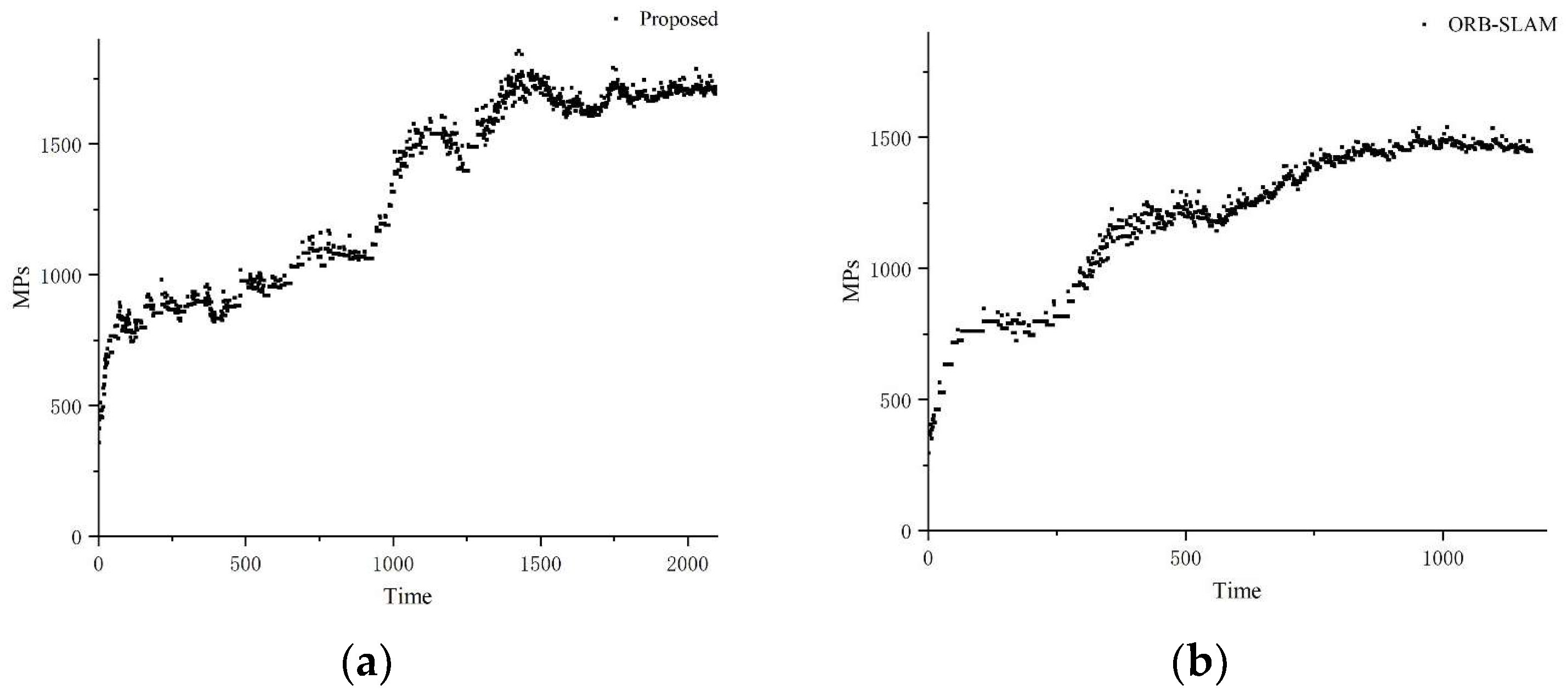
The number of mapping points (MPs) and keyframes (KFs) under both systems is shown in Figure 16 and Figure 17, respectively. The statistical results of mapping points and keyframes are shown in Table 7 and Table 8, respectively. The length of available data under the proposed system is 2167, and the length of available data under ORB-SLAM3 is 1171. It means the proposed system has a faster initialization than ORB-SLAM3 with the same datasets captured in the underwater raised sediments environment. The number of mapping points improved by 11.5%, and the number of mapping points improved by 5.2%. More matching point pairs provide more rich information for the mapping phase resulting in more mapping points obtained. The number of keyframes has increased less because the selection of keyframes is rigorous. More mapping points and keyframes mean the proposed system has robustness in the underwater raised sediments environment.
5. Conclusions
The underwater images are classified by the improved color recognition method to reduce the computation of image pre-processing to improve the real-time of the proposed SLAM system. The improved adaptive median filtering is proposed to denoise the classified images to reduce the effect of underwater raised sediments on feature matching of the SLAM system to improve the robustness of the proposed SLAM system. The MG of the filtered images is improved by 106.7% compared with those filtered by the traditional adaptive median filtering, SSIM by 4.6%, and PSNR by 1.1%, resulting in more information on the original features being retained compared with the traditional adaptive median filter. The filtered images are finally processed by the tracking module to obtain the trajectory of underwater vehicles and the seafloor maps. The datasets of the video captured from the seamount of the western Pacific Ocean at 3000 m depth are processed in the improved visual SLAM system. Keyframes, mapping points, and feature point matching pairs are extracted from the improved visual SLAM system by 5.2%, 11.2%, and 4.5% compared with ORB-SLAM3, respectively. The improved visual SLAM system has robustness in near-bottom environments such as seamounts, rockfall, and nodules, which is less impacted by dynamic disturbances such as water bubbles and underwater raised sediments.
In future work, the parameters of image classification and image denoising are adaptive for different underwater investigation tasks. The parameters of the proposed method are prior and set by the known underwater operating environments and the mounting locations of cameras. However, it is difficult to cope with an unknown environment underwater. The proposed SLAM is a loose-coupling system, in which the visual localization is realized by the pre-processed images imported into the tracking methods. The tight-coupling system will be studied in future work, in which the impact of underwater raised sediments is reduced by optimizing the feature matching phase within SLAM.
Author Contributions
This study is the result of collaborative teamwork. Conceptualization, Z.L. and M.W.; validation, Z.L.; writing—original draft preparation, Z.L.; writing—review and editing, M.W. and R.M.; supervision, H.H. and T.G. All authors have read and agreed to the published version of the manuscript.
Funding
The research carried out in this paper was partly supported by the National Natural Science Foundation of China with grant No. 52231011, 71971139.
Institutional Review Board Statement
Not applicable.
Informed Consent Statement
Not applicable.
Data Availability Statement
Data are contained within the article.
Conflicts of Interest
The authors declare no conflicts of interest.
References
- Mattioli, M.; Bernini, T.; Massari, G.; Lardeux, M.; Gower, A.; De Baermaker, S. Unlocking Resident Underwater Inspection Drones or AUV for subsea autonomous inspection: Value creation between technical requirements and technological development. In Proceedings of the Offshore Technology Conference, Houston, TX, USA, 2–5 May 2022; p. D021S024R004. [Google Scholar]
- Marini, S.; Gjeci, N.; Govindaraj, S.; But, A.; Sportich, B.; Ottaviani, E.; Márquez, F.P.G.; Bernalte Sanchez, P.J.; Pedersen, J.; Clausen, C.V. ENDURUNS: An integrated and flexible approach for seabed survey through autonomous mobile vehicles. J. Mar. Sci. Eng. 2020, 8, 633. [Google Scholar] [CrossRef]
- Vamråk Solheim, A.; Lesage, M.; Asbjørnslett, B.E.; Erikstad, S.O. Deep sea mining: Towards conceptual design for underwater transportation. In Proceedings of the International Conference on Offshore Mechanics and Arctic Engineering, Fort Lauderdale, FL, USA, 28 June–3 July 2020; p. V06BT06A050. [Google Scholar]
- Wang, Y.; Gu, D.; Ma, X.; Wang, J.; Wang, H. Robust real-time AUV self-localization based on stereo vision-inertia. IEEE Trans. Veh. Technol. 2023, 72, 7160–7170. [Google Scholar] [CrossRef]
- Hong, L.; Wang, X.; Zhang, D.-S.; Zhao, M.; Xu, H. Vision-Based Underwater Inspection with Portable Autonomous Underwater Vehicle: Development, Control, and Evaluation. IEEE Trans. Intell. Veh. 2023, 9, 2197–2209. [Google Scholar] [CrossRef]
- Chemisky, B.; Menna, F.; Nocerino, E.; Drap, P. Underwater survey for oil and gas industry: A review of close range optical methods. Remote Sens. 2021, 13, 2789. [Google Scholar] [CrossRef]
- Stenius, I.; Folkesson, J.; Bhat, S.; Sprague, C.I.; Ling, L.; Özkahraman, Ö.; Bore, N.; Cong, Z.; Severholt, J.; Ljung, C. A system for autonomous seaweed farm inspection with an underwater robot. Sensors 2022, 22, 5064. [Google Scholar] [CrossRef] [PubMed]
- Chen, W.; Shang, G.; Ji, A.; Zhou, C.; Wang, X.; Xu, C.; Li, Z.; Hu, K. An overview on visual slam: From tradition to semantic. Remote Sens. 2022, 14, 3010. [Google Scholar] [CrossRef]
- Sun, C.-Z.; Zhang, B.; Wang, J.-K.; Zhang, C.-S. A review of visual SLAM based on unmanned systems. In Proceedings of the 2021 2nd International Conference on Artificial Intelligence and Education (ICAIE), Dali, China, 18–20 June 2021; pp. 226–234. [Google Scholar]
- Wu, Y.; Ta, X.; Xiao, R.; Wei, Y.; An, D.; Li, D. Survey of underwater robot positioning navigation. Appl. Ocean Res. 2019, 90, 101845. [Google Scholar] [CrossRef]
- Zhang, X.; He, B.; Gao, S.; Mu, P.; Xu, J.; Zhai, N. Multiple model AUV navigation methodology with adaptivity and robustness. Ocean Eng. 2022, 254, 111258. [Google Scholar] [CrossRef]
- Wang, Y.; Huang, S.; Wang, Z.; Hu, R.; Feng, M.; Du, P.; Yang, W.; Chen, Y. Design and experimental results of passive iUSBL for small AUV navigation. Ocean Eng. 2022, 248, 110812. [Google Scholar] [CrossRef]
- Song, Z.; Bian, H.; Zielinski, A. Application of acoustic image processing in underwater terrain aided navigation. Ocean Eng. 2016, 121, 279–290. [Google Scholar] [CrossRef]
- Xu, C.; Xu, C.; Wu, C.; Qu, D.; Liu, J.; Wang, Y.; Shao, G. A novel self-adapting filter based navigation algorithm for autonomous underwater vehicles. Ocean Eng. 2019, 187, 106146. [Google Scholar] [CrossRef]
- Zhang, X.; He, B.; Mu, P.; Zhang, D. Hybrid model navigation method for autonomous underwater vehicle. Ocean Eng. 2022, 261, 112027. [Google Scholar] [CrossRef]
- Lv, P.-F.; He, B.; Guo, J.; Shen, Y.; Yan, T.-H.; Sha, Q.-X. Underwater navigation methodology based on intelligent velocity model for standard AUV. Ocean Eng. 2020, 202, 107073. [Google Scholar] [CrossRef]
- Xu, Z.; Haroutunian, M.; Murphy, A.J.; Neasham, J.; Norman, R. A Low-Cost Visual Inertial Odometry System for Underwater Vehicles. In Proceedings of the 2021 4th International Conference on Mechatronics, Robotics and Automation (ICMRA), Zhanjiang, China, 22–24 October 2021; pp. 139–143. [Google Scholar]
- Qin, J.; Li, M.; Li, D.; Zhong, J.; Yang, K. A survey on visual navigation and positioning for autonomous UUVs. Remote Sens. 2022, 14, 3794. [Google Scholar] [CrossRef]
- Köser, K.; Frese, U. Challenges in underwater visual navigation and SLAM. In AI Technology for Underwater Robots; Springer: Cham, Switzerland, 2020; pp. 125–135. [Google Scholar]
- Carreras, M.; Hernández, J.D.; Vidal, E.; Palomeras, N.; Ribas, D.; Ridao, P. Sparus II AUV—A hovering vehicle for seabed inspection. IEEE J. Ocean Eng. 2018, 43, 344–355. [Google Scholar] [CrossRef]
- Abu, A.; Diamant, R. A SLAM Approach to Combine Optical and Sonar Information from an AUV. IEEE Trans. Mob. Comput. 2023, 1–11. [Google Scholar] [CrossRef]
- Özkahraman, Ö.; Ögren, P. Efficient navigation aware seabed coverage using auvs. In Proceedings of the 2021 IEEE International Symposium on Safety, Security, and Rescue Robotics (SSRR), New York, NY, USA, 25–27 October 2021; pp. 63–70. [Google Scholar]
- Sabra, A. Cooperative Localisation in Underwater Robotic Swarms for Ocean Bottom Seismic Imaging. Ph.D. Thesis, Robert Gordon University, Aberdeen, UK, 2021. [Google Scholar]
- Issartel, M. Towards a Robust Slam Framework for Resilient AUV Navigation. Ph.D. Thesis, Cranfield University, Bedford, UK, 2021. [Google Scholar]
- Zhang, Q.; Li, Y.; Ma, T.; Cong, Z.; Zhang, W. Bathymetric particle filter SLAM based on mean trajectory map representation. IEEE Access 2021, 9, 71725–71736. [Google Scholar] [CrossRef]
- Xu, W.; Yang, J.; Wei, H.; Lu, H.; Tian, X.; Li, X. A localization algorithm based on pose graph using Forward-looking sonar for deep-sea mining vehicle. Ocean Eng. 2023, 284, 114968. [Google Scholar] [CrossRef]
- Mahajan, A.; Rock, S. A Pilot Aid for Real-Time Vision-Based Coverage Estimation for Seabed Surveying Applications. In Proceedings of the Global Oceans 2020: Singapore–US Gulf Coast, Biloxi, MS, USA, 5–30 October 2020; pp. 1–6. [Google Scholar]
- Joshi, B.; Rahman, S.; Kalaitzakis, M.; Cain, B.; Johnson, J.; Xanthidis, M.; Karapetyan, N.; Hernandez, A.; Li, A.Q.; Vitzilaios, N. Experimental comparison of open source visual-inertial-based state estimation algorithms in the underwater domain. In Proceedings of the 2019 IEEE/RSJ International Conference on Intelligent Robots and Systems (IROS), Macau, China, 3–8 November 2019; pp. 7227–7233. [Google Scholar]
- Bonin-Font, F.; Oliver, G.; Wirth, S.; Massot, M.; Negre, P.L.; Beltran, J.-P. Visual sensing for autonomous underwater exploration and intervention tasks. Ocean Eng. 2015, 93, 25–44. [Google Scholar] [CrossRef]
- Wang, T.; Zhao, Q.; Yang, C. Visual navigation and docking for a planar type AUV docking and charging system. Ocean Eng. 2021, 224, 108744. [Google Scholar] [CrossRef]
- Ferrera, M.; Moras, J.; Trouvé-Peloux, P.; Creuze, V. Real-time monocular visual odometry for turbid and dynamic underwater environments. Sensors 2019, 19, 687. [Google Scholar] [CrossRef]
- Cheng, J.; Zhang, L.; Chen, Q.; Hu, X.; Cai, J. A review of visual SLAM methods for autonomous driving vehicles. Eng. Appl. Artif. Intell. 2022, 114, 104992. [Google Scholar] [CrossRef]
- Mittal, S.; Srivastava, S.; Jayanth, J.P. A survey of deep learning techniques for underwater image classification. IEEE Trans. Neural Netw. Learn. Syst. 2022, 34, 6968–6982. [Google Scholar] [CrossRef]
- Mahmood, A.; Bennamoun, M.; An, S.; Sohel, F.; Boussaid, F. ResFeats: Residual network based features for underwater image classification. Image Vis. Comput. 2020, 93, 103811. [Google Scholar] [CrossRef]
- Lopez-Vazquez, V.; Lopez-Guede, J.M.; Marini, S.; Fanelli, E.; Johnsen, E.; Aguzzi, J. Video image enhancement and machine learning pipeline for underwater animal detection and classification at cabled observatories. Sensors 2020, 20, 726. [Google Scholar] [CrossRef]
- Goyal, B.; Dogra, A.; Agrawal, S.; Sohi, B.S.; Sharma, A. Image denoising review: From classical to state-of-the-art approaches. Inf. Fusion 2020, 55, 220–244. [Google Scholar] [CrossRef]
- Tian, C.; Fei, L.; Zheng, W.; Xu, Y.; Zuo, W.; Lin, C.-W. Deep learning on image denoising: An overview. Neural Netw. 2020, 131, 251–275. [Google Scholar] [CrossRef]
- Pang, T.; Zheng, H.; Quan, Y.; Ji, H. Recorrupted-to-recorrupted: Unsupervised deep learning for image denoising. In Proceedings of the IEEE/CVF Conference on Computer Vision and Pattern Recognition, Nashville, TN, USA, 20–25 June 2021; pp. 2043–2052. [Google Scholar]
- Li, J.; Zhang, Z.; Liu, X.; Feng, C.; Wang, X.; Lei, L.; Zuo, W. Spatially Adaptive Self-Supervised Learning for Real-World Image Denoising. In Proceedings of the IEEE/CVF Conference on Computer Vision and Pattern Recognition, Vancouver, BC, Canada, 17–24 June 2023; pp. 9914–9924. [Google Scholar]
- Dasari, S.K.; Sravani, L.; Kumar, M.U.; Rama Venkata Sai, N. Image Enhancement of Underwater Images Using Deep Learning Techniques. In Proceedings of the International Conference on Data Analytics and Insights, Kolkata, India, 11–13 May 2023; pp. 715–730. [Google Scholar]
- Raj, M.V.; Murugan, S.S. Underwater image classification using machine learning technique. In Proceedings of the 2019 International Symposium on Ocean Technology (SYMPOL), Ernakulam, India, 11–13 December 2019; pp. 166–173. [Google Scholar]
- Moghimi, M.K.; Mohanna, F. Real-time underwater image resolution enhancement using super-resolution with deep convolutional neural networks. J. Real-Time Image Process. 2021, 18, 1653–1667. [Google Scholar] [CrossRef]
- Fan, L.; Zhang, F.; Fan, H.; Zhang, C. Brief review of image denoising techniques. Vis. Comput. Ind. Biomed. Art 2019, 2, 1–12. [Google Scholar] [CrossRef]
- Kumar, N.; Dahiya, A.K.; Kumar, K. Modified median filter for image denoising. Int. J. Adv. Sci. Technol. 2020, 29, 1495–1502. [Google Scholar]
- Sagar, P.; Upadhyaya, A.; Mishra, S.K.; Pandey, R.N.; Sahu, S.S.; Panda, G. A circular adaptive median filter for salt and pepper noise suppression from MRI images. J. Sci. Ind. Res. 2020, 79, 941–944. [Google Scholar]
Figure 1.
No raised sediment environment in the underwater area. (a) The seamount area; (b) the rockfall area; and (c) the nodules area.
Figure 1.
No raised sediment environment in the underwater area. (a) The seamount area; (b) the rockfall area; and (c) the nodules area.

Figure 2.
Different degrees of the raised sediments in different areas. (a) Light degree in the seamount area; (b) medium degree in the rockfall area; and (c) heavy degree in the nodules area.
Figure 2.
Different degrees of the raised sediments in different areas. (a) Light degree in the seamount area; (b) medium degree in the rockfall area; and (c) heavy degree in the nodules area.

Figure 3.
The block diagram of the improved underwater visual SLAM system.

Figure 4.
The flowchart of the proposed image classification method.

Figure 5.
The flowchart of the improved adaptive median filtering method.

Figure 6.
The pixel value of window length .

Figure 7.
The sequence of window length .

Figure 8.
The mean gray value of the window border.

Figure 9.
Improved adaptive median filtering results in the seamount area. (a) Original color image; (b) original grayscale image; (c) traditional adaptive median filtering; and (d) improved adaptive median filtering.
Figure 9.
Improved adaptive median filtering results in the seamount area. (a) Original color image; (b) original grayscale image; (c) traditional adaptive median filtering; and (d) improved adaptive median filtering.

Figure 10.
Initialization failure under ORB-SLAM3 system. (a) Initialization failure in Test 1. (b) Initialization failure in Test 2.
Figure 10.
Initialization failure under ORB-SLAM3 system. (a) Initialization failure in Test 1. (b) Initialization failure in Test 2.

Figure 11.
Initialization success under the proposed system. (a) Initialization success in Test 1. (b) Initialization success in Test 2.
Figure 11.
Initialization success under the proposed system. (a) Initialization success in Test 1. (b) Initialization success in Test 2.

Figure 12.
Mapping and trajectory in the initialization phase under the proposed system. (a) Moment 1. (b) Moment 2.
Figure 12.
Mapping and trajectory in the initialization phase under the proposed system. (a) Moment 1. (b) Moment 2.

Figure 13.
Mapping and trajectory in the end phase under the ORB-SLAM3 system. (a) Moment 1. (b) Moment 2.
Figure 13.
Mapping and trajectory in the end phase under the ORB-SLAM3 system. (a) Moment 1. (b) Moment 2.

Figure 14.
Mapping and trajectory in the end phase under the proposed system. (a) Moment 1. (b) Moment 2.
Figure 14.
Mapping and trajectory in the end phase under the proposed system. (a) Moment 1. (b) Moment 2.

Figure 15.
The number of match point pairs under both systems. (a) The proposed system. (b) ORB-SLAM3 system.
Figure 15.
The number of match point pairs under both systems. (a) The proposed system. (b) ORB-SLAM3 system.

Figure 16.
The number of mapping points under both systems. (a) The proposed system. (b) ORB-SLAM3 system.
Figure 16.
The number of mapping points under both systems. (a) The proposed system. (b) ORB-SLAM3 system.

Figure 17.
The number of keyframes under both systems. (a) The proposed system. (b) ORB-SLAM3 system.
Figure 17.
The number of keyframes under both systems. (a) The proposed system. (b) ORB-SLAM3 system.


Table 1.
Classification results of the 2000 underwater images in the seamounts area.
| Discriminant Threshold | Need-Denoising | Original | Accuracy |
|---|---|---|---|
| 10 | 868 | 1132 | 75.4% |
| 15 | 454 | 1546 | 96.1% |
| 20 | 296 | 1704 | 95.9% |
| 25 | 112 | 1888 | 86.7% |
| 30 | 23 | 1977 | 82.3% |
| Real | 377 | 1623 | - |
Table 2.
Classification results of the 2000 underwater images in the rockfall area.
| Discriminant Threshold | Need-Denoising | Original | Accuracy |
|---|---|---|---|
| 10 | 1267 | 733 | 64.8% |
| 15 | 942 | 1158 | 81.1% |
| 20 | 603 | 1704 | 98.0% |
| 25 | 430 | 1570 | 93.4% |
| 30 | 224 | 1776 | 83.1% |
| Real | 563 | 1437 | - |
Table 3.
Classification results of the 2000 underwater images in the nodules area.
| Discriminant Threshold | Need-Denoising | Original | Accuracy |
|---|---|---|---|
| 10 | 184 | 1816 | 84.8% |
| 15 | 112 | 1888 | 81.2% |
| 20 | 47 | 1953 | 78.0% |
| 25 | 32 | 1968 | 77.2% |
| 30 | 2 | 1998 | 75.7% |
| Real | 488 | 1437 | - |
Table 4.
Image quality assessment results in the seamount area.
| Metrics | TAMF | IAMF | Improvement |
|---|---|---|---|
| MG | 1.3761 | 2.8451 | 106.7% |
| SSIM | 0.9164 | 0.9591 | 4.6% |
| PSNR | 81.60 | 85.10 | 1.1% |
Table 5.
Experimental test environment for the seamount images.
| Related Devices | Model |
|---|---|
| Visual SLAM | ORB-SLAM3 |
| SLAM operating system | Ubuntu 20.04 |
| Image processing operating system | Windows 10 |
| Image processing program software | MatLab R2022a |
| CPU | Ryzen7 |
Table 6.
Statistical results of match point pairs.
| Number | ORB-SLAM3 | Proposed |
|---|---|---|
| Max | 503 | 490 |
| Min | 82 | 90 |
| Average | 292.05 | 305.14 |
| Improvement | - | 4.5% |
Table 7.
Statistical results of mapping points.
| Number | ORB-SLAM3 | Proposed |
|---|---|---|
| Max | 1538 | 1855 |
| Min | 296 | 358 |
| Average | 1181.06 | 1316.59 |
| Improvement | - | 11.5% |
Table 8.
Statistical results of keyframes.
| Number | ORB-SLAM3 | Proposed |
|---|---|---|
| Max | 36 | 38 |
| Min | 3 | 3 |
| Average | 21.30 | 22.42 |
| Improvement | - | 5.2% |
Disclaimer/Publisher’s Note: The statements, opinions and data contained in all publications are solely those of the individual author(s) and contributor(s) and not of MDPI and/or the editor(s). MDPI and/or the editor(s) disclaim responsibility for any injury to people or property resulting from any ideas, methods, instructions or products referred to in the content. |
© 2024 by the authors. Licensee MDPI, Basel, Switzerland. This article is an open access article distributed under the terms and conditions of the Creative Commons Attribution (CC BY) license (https://creativecommons.org/licenses/by/4.0/).
Share and Cite
MDPI and ACS Style
Liu, Z.; Wang, M.; Hu, H.; Ge, T.; Miao, R. An Underwater Localization Method Based on Visual SLAM for the Near-Bottom Environment. J. Mar. Sci. Eng. 2024, 12, 716. https://0-doi-org.brum.beds.ac.uk/10.3390/jmse12050716
AMA Style
Liu Z, Wang M, Hu H, Ge T, Miao R. An Underwater Localization Method Based on Visual SLAM for the Near-Bottom Environment. Journal of Marine Science and Engineering. 2024; 12(5):716. https://0-doi-org.brum.beds.ac.uk/10.3390/jmse12050716
Chicago/Turabian StyleLiu, Zonglin, Meng Wang, Hanwen Hu, Tong Ge, and Rui Miao. 2024. "An Underwater Localization Method Based on Visual SLAM for the Near-Bottom Environment" Journal of Marine Science and Engineering 12, no. 5: 716. https://0-doi-org.brum.beds.ac.uk/10.3390/jmse12050716
Note that from the first issue of 2016, this journal uses article numbers instead of page numbers. See further details here.