


Artificial Neural Networks for Mapping Coastal Lagoon of Chilika Lake, India, Using Earth Observation Data


Department of Geoinformatics, Faculty of Digital and Analytical Sciences, Universität Salzburg, Schillerstraße 30, A-5020 Salzburg, Austria
J. Mar. Sci. Eng. 2024, 12(5), 709; https://0-doi-org.brum.beds.ac.uk/10.3390/jmse12050709
Submission received: 5 March 2024
/
Revised: 16 April 2024
/
Accepted: 23 April 2024
/
Published: 25 April 2024
(This article belongs to the Special Issue Remote Sensing Applications in Marine Environmental Monitoring)
Abstract
:This study presents the environmental mapping of the Chilika Lake coastal lagoon, India, using satellite images Landsat 8-9 OLI/TIRS processed using machine learning (ML) methods. The largest brackish water coastal lagoon in Asia, Chilika Lake, is a wetland of international importance included in the Ramsar site due to its rich biodiversity, productivity, and precious habitat for migrating birds and rare species. The vulnerable ecosystems of the Chilika Lagoon are subject to climate effects (monsoon effects) and anthropogenic activities (overexploitation through fishing and pollution by microplastics). Such environmental pressure results in the eutrophication of the lake, coastal erosion, fluctuations in size, and changes in land cover types in the surrounding landscapes. The habitat monitoring of the coastal lagoons is complex and difficult to implement with conventional Geographic Information System (GIS) methods. In particular, landscape variability, patch fragmentation, and landscape dynamics play a crucial role in environmental dynamics along the eastern coasts of the Bay of Bengal, which is strongly affected by the Indian monsoon system, which controls the precipitation pattern and ecosystem structure. To improve methods of environmental monitoring of coastal areas, this study employs the methods of ML and Artificial Neural Networks (ANNs), which present a powerful tool for computer vision, image classification, and analysis of Earth Observation (EO) data. Multispectral satellite data were processed by several ML image classification methods, including Random Forest (RF), Support Vector Machine (SVM), and the ANN-based MultiLayer Perceptron (MLP) Classifier. The results are compared and discussed. The ANN-based approach outperformed the other methods in terms of accuracy and precision of mapping. Ten land cover classes around the Chilika coastal lagoon were identified via spatio-temporal variations in land cover types from 2019 until 2024. This study provides ML-based maps implemented using Geographic Resources Analysis Support System (GRASS) GIS image analysis software and aims to support ML-based mapping approach of environmental processes over the Chilika Lake coastal lagoon, India.
1. Introduction
1.1. Background
Coastal lagoons play a key role in the hydrological and ecological processes in the zones between land and sea. They distribute and diversify riverine sediments [1], reduce turbulence of tidal flow [2], regulate seasonal current water circulation [3], and enrich shelf waters with nutrients [4]. Worldwide, coastal lagoons are among the most productive and biodiverse systems, providing essential habitat for a wide variety of aquatic species and threatened marine fauna [5,6,7]. Coastal and brackish water lagoons that form continuities in the terrestrial and shelf ecosystems present transitional aquatic ecosystems located in the zones between land and sea. They are often associated with dynamic environmental conditions and high biodiversity due to their connections to the marine and terrestrial communities [8].
Formed as a result of the marine transgression, coastal lagoons vary with depth and geomorphic features, tidal circulation patterns, salinity, and wind forcing [9]. The formation of the barriers between the land and ocean is driven by the controversial forces of erosion and sediment deposition within the coastal lagoons [10]. The accumulation of river sediments depends on the speed of the river that enters the coastal lagoon and transports sediments in large quantities. Furthermore, complex hydrological processes such as winds, oceanic currents, and coastal waves, as well as groundwater discharge [11], intensify the mixing of sediments and nutrients within the coastal lagoons [12]. Moreover, different slope and substrate types and density-driven currents with diverse morphodynamic tidal regimes affect littoral zones and create stratified conditions of sediment resuspension [13,14].
Topographically isolated and hydrologically distinct from the surrounding landscapes, coastal lagoons include unique species of wild flora and fauna (e.g., bird species). The transitional location of the coastal lagoons determines their high levels of biodiversity through the intense physical–chemical gradients. A particular feature of the coastal lagoons that ensures their high productivity as aquatic systems is their shallow bathymetry [15]. The water mass of the lagoon is well mixed because the sunlight reaches all levels of the shallow systems of the coastal lagoons until the lowest bottom layer of water due to the active waves and currents. Such dynamics activate the recycling of nutrients and increase biological productivity [16]. They have been declared as marine protected areas worldwide due to their rich bioproductivity and valuable environment.
However, recent monitoring has indicated their decline, habitat loss, and environmental vulnerability [17,18,19]. These declines have been attributed to a variety of indirect and direct causes, including climate change [20] and anthropogenic activities with their associated pollution [21]. High levels of stress result in environmental threats to these treasured ecosystems [22]. Among recent environmental problems of coastal lagoons are affected biodiversity patterns and loss of habitats and rare species [23,24], as well as disrupted land cover patterns due to climate effects. Examples of pollution include organic, chemical, and biological types such as microplastic [25,26] or heavy metals [27].
The transitional nature of coastal lagoons makes them vulnerable to the cumulative effects from climate fluctuations, specifically rising sea levels [28], flooding [29], hydrological disturbances, nutrient availability [30], and human impacts [31]. The richness in natural resources of coastal lagoons attracts the local population and urges them to actively use the resources of the aquatic environment. Hence, coastal lagoons serve as a valuable source of food and natural resources and support economic development and sustainability for the local population. In turn, this leads to the overexploitation of these unique areas and increases anthropogenic pressure [32].
1.2. Objective and Goal
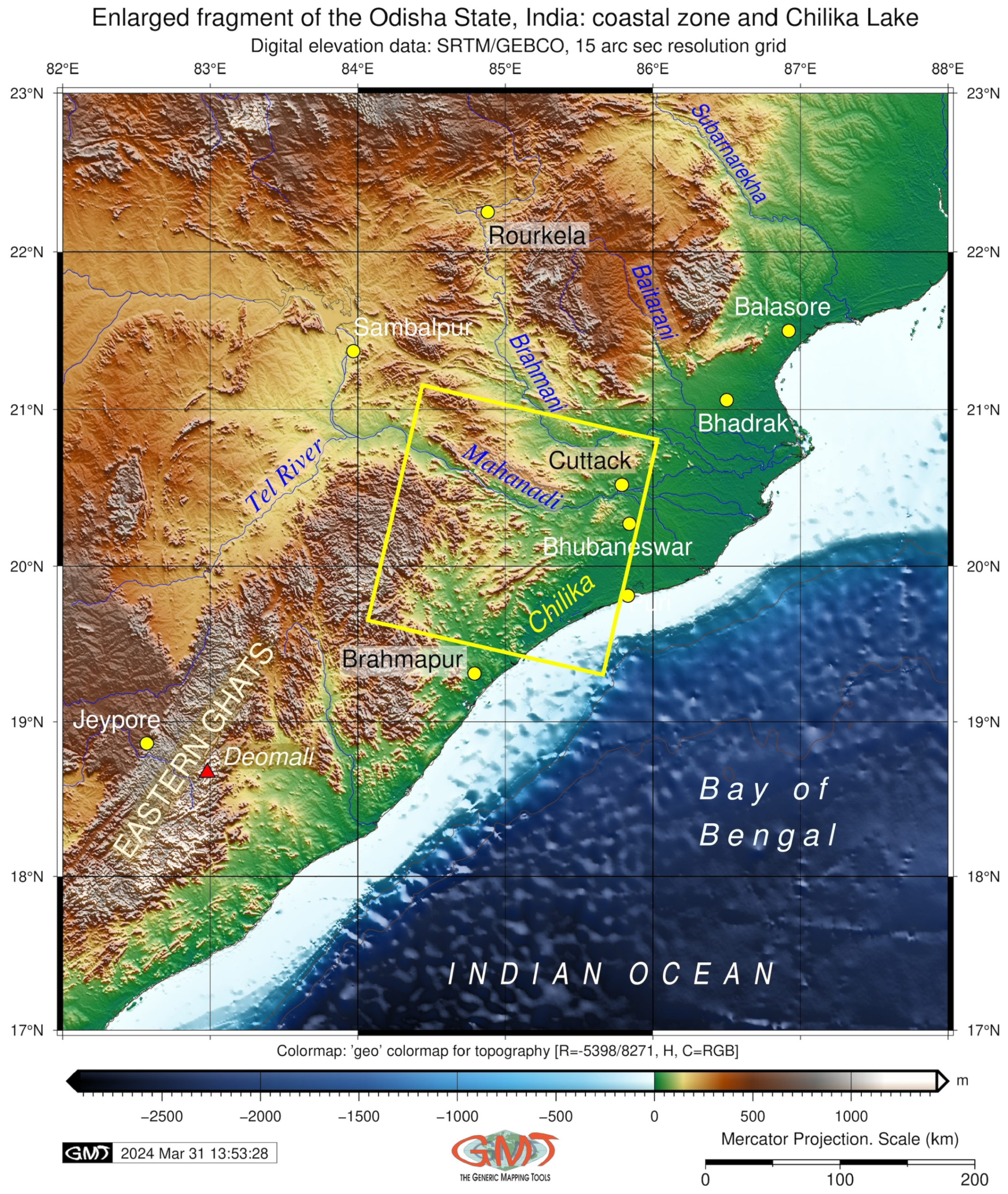
The main goal of this research is to map and analyze changes in the land cover types surrounding the coastal lagoon on the lake using machine learning (ML) algorithms using Geographic Resources Analysis Support System (GRASS) GIS and Earth Observation (EO) data. We used Landsat 8-9 OLI/TIRS satellite images from recent six years (2019, 2020, 2021, 2022, 2023 and 2024) and processed them using ANN and ML methods to analyze the spatio-temporal distribution of land cover types in Chilika coastal lagoon, Bay of Bengal, India (Figure 1). To set up the advanced practical background for the environmental analysis of Chilika Lake, this study presents an ML approach for the automation of EO data processing, classification, and visualization. To achieve this goal, the objective is to use the ANN methods from Python’s library Scikit-Learn version 1.4.2 [33], which are embedded in the GRASS GIS version 8.3 [34] through ML modules designed for data partition and satellite image processing.
The ML approach was selected since it creates a plausible paradigm to map the environmental variability of the coastal landscapes surrounding the lagoon of Chilika Lake. Among the existing methods, this study employs the MultiLayer Perceptron (MLP) algorithm of ANN, which presents an effective solution to image analysis.
1.3. Research Gap
There is little research analyzing and contrasting landscapes of the Odisha coasts using the ML approach. Existing studies draw generalizations regarding the links between the ecosystems of the coastal lagoon of Chilika Lake and the adjacent habitat communities [35,36,37,38]. However, they utilize the conventional tools of cartographic software, which applies traditional mapping methods. To the best of our knowledge, no reported research has been carried out using ANN techniques to study the environmental variability of Chilika Lake with a spatial extent with the coordinates of 19°28′–19°54′ N; 85°06′–85°35′ E; see Figure 2.
At the same time, ANN methods and scripting libraries are promising tools for cartographic tasks and image processing for mapping areas of coastal lagoons, which are notable for the high complexity of land cover patterns and the heterogeneity of landscapes [39,40,41,42,43,44]. In this regard, GRASS GIS presents a powerful cartographic toolset that includes diverse modules that can be used for satellite image processing [45]. Hence, besides the traditional general-purpose programming languages, GRASS GIS is also used for creation. Hence, ML applications in cartography provide insight into its spatio-temporal variability of landscapes and environmental processes through the classification of the EO data [46,47,48,49].
1.4. Theoretical Framework and Motivation
Monitoring coastal landscapes and variations in land cover types around coastal lagoons is essential for land management and conservation activities of the Chilika Lake. Such activities are carried out and reported in previous studies based on conventional mapping. Nevertheless, monitoring land cover types in a lake using traditional methods is often time-consuming and labor-intensive and includes considerable manual work, which is prone to errors. Though mapping using Geographic Information System (GIS) presents a reliable solution to Earth Observation (EO) data processing, estimation accuracy is still a notable challenge in mapping coastal areas with high heterogeneity of land cover types. Due to the logical straightforwardness of the classification algorithms, their application for thematic GIS-based mapping and analysis of landscape dynamics presents a well-known approach to cartographic workflow with existing case studies on Chilika Lake, the Mahanadi Delta, and the Odisha coastal area [50,51,52,53].
However, the spectral complexity of the multispectral satellite images makes recognizing land cover types in coastal areas a challenging and less accurate task using k-means clustering or “MaxLike” classification. For instance, specifically for lagoons, the optical properties of coastal waters and shelf areas are significantly affected by the suspended sediment from the colored dissolved organic matter (CDOM), which can create noise on the EO data. On the other hand, the classification of the EO data using machine learning (ML) methods has been fairly successful. For example, to solve these issues, ML algorithms present automation of image classification [54,55], which is achieved through computer vision algorithms of pattern recognition and analysis that enables the recognition of geometrical complexity [48].
The application of ML methods based on the Artificial Neural Networks (ANNs) applied to Remote Sensing (RS) data processing considerably increases the effectiveness of mapping [56,57]. Advanced ML methods enable the landscape dynamics of spatial and temporal trends to be automatically revealed through computer-based algorithms of pattern recognition and data analysis, as reported in existing studies [58,59,60,61,62]. Several ML and AI algorithms exist to analyze and quantify spatial data using analytical and empirical approaches. Their main approach includes neural networks that teach computers to process data in an analytical way that simulates the human brain in pattern recognition [63,64]. Among the advanced ML algorithms are the Random Forest (RF) [65], Support Vector Machines (SVMs) [66], and Naive Bayes [67], to mention a few. In this study, we use such algorithms for processing RS data. The goal of this approach is to perform satellite image classification with a case study of Chilika Lake coastal lagoon, East India.
2. Study Area
The study area covers a spatial extent with the coordinates of 19°28′–19°54′ N; 85°06′–85°35′ E, [68] located in the state of Odisha, East India, Figure 3.
The largest brackish water lagoon in Asia [69,70], Chilika Lake covers a total area of over with existing fluctuations of the lake surface reported between and [71]. The lake is located at the junction of two different water masses—riverine freshwater and oceanic salt waters from the tidal influx of the Bay of Bengal. Different water fronts interact with the bathymetry of the lagoon and generate local hydrographic settings, which causes local variations in salinity, current turbulence, and circular flow patterns of waves [72]. The coastal lagoon formed by the Chilika Lake lies at the estuary of the Daya River, which enters the Bay of Bengal on the east coast of India; see Figure 3.
A recent geological study has shown that the shallow limnological system of Chilika Lake was a part of the Bay of Bengal during the later stages of the Pleistocene period [73], and underwent marked geomorphic evolution during the late Holocene [74,75]. This included significant denudation and weathering of the surrounding coasts. Such processes are mostly caused by climate variability and accelerated by the effects of monsoon cycles, which influence the distribution of mangroves [76] and other vegetation types around the lake and estuarine environment [77]. Currently, the dynamics of the surface area in the coastal lagoon of Chilika Lake present a response to the cumulative effects of tidal morphodynamics, winds, and morphometry. The integrating forces of these processes resulted in fluctuating surface and area, which affect the ecosystem of the surrounding wetlands.
The coastal lagoon of the Chilika Lake has important conservation features. These include, for instance, rare aquatic and sub-aquatic plants, endemic species, mangrove associations, and plants of horticultural importance. The significant biodiversity and ecosystem value of the Chilika Lake can be illustrated by the impressive number of species, which exceeds 300 fish species [78] and 726 species of flowering plants [79]. Moreover, Chilika Lake is the largest habitat for migratory waterbirds across India and a home to multiple threatened and rare species, including both plants and animals [80].
Such rich natural resources and the unique environment of Chilika Lake have attracted humans to this area since the ancient period. Archaeological records prove that human settlements existed in the Chilika Lake area since at least the Neolithic period when this area served as a marine harbor and port [81]. The attractiveness of Chilika Lake is explained by its favorable climate, beneficial topographic setting, and strategic location, which have given access to the Indian Ocean and ensure safe maritime trade and international commercial connections in India since the ancient period. The importance of the Chilika Lake both ecologically and historically in the development of Indian civilization resulted in its official designation a as UNESCO World Heritage site [82] and a Ramsar site [83].
3. Materials and Methods
3.1. Data
Spatial analysis was limited to RS data using multispectral satellite images Landsat. A time series of satellite images collected at regular time intervals and covering the study area is a key instrument for environmental analysis [84]. To this end, six satellite images were collected during the spring period (February–March) and covering the time interval of 2019 to 2024. All but two datasets (early March 2020 and early March 2023) were acquired within the period of February (that is, images on 2019, 2021, 2022, and 2024), when the aquatic and coastal vegetation around the lagoon is typically well developed prior to the pre-monsoon decline during the period from April to June and monsoon rains, which last in India from June to September. Hence, the images were taken on the following dates: 13 February 2019, 3 March 2020, 2 February 2021, 13 February 2022, 4 March 2023 and 11 February 2024.
Water turbidity is relatively low during the late winter to early spring period due to seasonally reduced rainfall in the “no monsoon” period. This allowed for the identification of land cover types through the satellite image analysis. Finally, the spring period enables the detection of algae blooms in the coastal lagoon, which usually occur in India from February to May (subject to climate fluctuations). Algae bloom in the coastal lagoon of Chilika Lake is caused by several factors such as the effects of monsoon cycles, riverine discharge, and seasonal upwelling. Hence, the images were selected for spring period with low cloudiness (below 10%) to increase the quality of image analysis.
The satellite data were obtained from the Landsat 8-9 OLI/TIRS mission and downloaded from the NASA EarthExplorer website (https://earthexplorer.usgs.gov/, accessed 3 March 2024). The original images are shown in Figure 4. Image frames acquired from EarthExplorer were imported to the GRASS GIS individually using extent and resolution corresponding to the multispectral bands, then pre-processed for top-of-atmosphere reflectance using the “i.landsat.toar” module. The major technical characteristics of the satellite images common for all the scenes are as follows. The images were obtained during the daytime in the nadir from sensor OLI/TIRS of Landsat Collection Category T1, Nr. 2. The Worldwide Reference System (WRS) Path/Row is 140/46. The images were projected into the Universal Transverse Mercator (UTM) projection Zone 45, Datum and Ellipsoid is World Geodetic System 84 (WGS84), Ground Control Points Version 5; Station Identifier LGN. The remaining technical characteristics of the EO data are summarized in Appendix A. Other geospatial data include the cartographic datasets: the raster topographic grid of the General Bathymetric Chart of the Oceans (GEBCO) and vector layers of the administrative division of India. These data were used to visualize the location of the region within the country at the state level, as well as the terrain of the study area.
3.2. Methodological Workflow
These data were processed using the GRASS GIS software version 8.3.1, Generic Mapping Tools (GMT) cartographic scripting toolset version 6.4.0 [85] and QGIS software version 3.34. The methodology used for mapping is derived from previous works [86,87,88]. The workflow of this study included several processes and approaches to image analysis and multi-source data, as summarized in the methodological scheme in Figure 5.
As such, combining RS data and machine learning (ML) techniques presents the integration of the two technologies that complement each other in the programming approach of GRASS GIS and help overcome the limitation of using just one. Moreover, the current focus on employing the ML methods for monitoring the coastal lagoon of the Chilika Lake underscores its important contribution to the modeling of the geospatial data. This approach to data processing supports the computer-based modeling of landscape dynamics in the coastal regions of the Bay of Bengal and helps analyze how these regions are affected by the environmental and climate variability in the monsoon climate of the Indian Ocean.
3.3. Image Processing
The images were processed using the GRASS GIS (v. 8.3) image processing software using methods explained in the following subsections. First, the images were imported and preprocessed. Then, the images were classified using the unsupervised clustering of the maximum-likelihood discriminant analysis classifier (MaxLik). During the clustering steps, the signature file was generated and reported using the k-means algorithm. The aim of this step is to perform cluster maps and to obtain a training dataset. The classification was performed by the ’i.maxlik’ module of GRASS GIS. The code for these steps is presented in Listing 1 using GRASS GIS syntax:
| Listing 1. GRASS GIS code for clustering method using k-means algorithm. |
 |
The visualization of the maps was performed using cartographic tools of GRASS GIS as follows in Listing 2:
| Listing 2. GRASS GIS code for mapping and cartographic display. |
 |
The next steps included machine learning (ML) algorithms for image processing and analysis by GRASS GIS.
3.4. Machine Learning
3.4.1. Random Forest
The mathematical foundation of the Random Forest (RF) classification consists of the following steps of the workflow initially developed by [65]. For to B, a bootstrap sample of size N from the training data has been drawn. Afterward, the random-forest tree is increased to the bootstrapped data. This is carried out iteratively by recursively repeating the logical steps for each terminal node of the tree that represents the individual class in land cover classification until the minimum node size min is reached.
The m variables are randomly selected using the data obtained in the “r.random” module of GRASS GIS obtained from the pixel variables “p”. The best variable and split point are then selected among the m, and the model splits each node into two “daughter” nodes. The output model of the ensemble of trees is received as . Then, to make a prediction of the assignment of each pixel within the matrix of the raster image to the specific land cover class, the model evaluates each new point x (that is, a cell on the satellite image) using the following logical expression. Let be the class prediction of the b-th random-forest tree. Then, the RF classification is performed by running Equation (1) derived from [89]:
The criteria for the RF model include the number of pixels forming the class (the spectral reflectance variability of vegetation and land categories). The optimal parameter was defined as 10 classes using existing similar studies. Second, the extent of the area in the pixel’s surrounding was set up according to the resolution of the Landsat images as 30 m per pixel around the target land cover class, forming the complete landscape pattern, plus including the pixels themselves evaluated for spectral reflectance using the ANN and ML methods. Hence, the RF classification obtains a class vote from each tree and then classifies it using majority vote and analysis of each pixel within the raster image. In GRASS GIS, the RF-based image classification is carried out using the code presented in Listing 1.
Here, the training pixels were first generated to train from an earlier land cover classification. Then, they were used as training datasets to perform a classification on recent Landsat images (in the example of code below, for the image of 2023). Afterwards, the model was trained using the “RandomForestClassifier” embedded algorithm using “r.learn.train” module. The prediction of the model’s performance was carried out using the “r.learn.predict” module. The shaded relief was added as a background to the image, and the isolines were derived using the “r.contour” module. The code is presented in Listing 3.
| Listing 3. GRASS GIS code for RF method for supervised image classification. |
 |
3.4.2. MultiLayer Perceptron
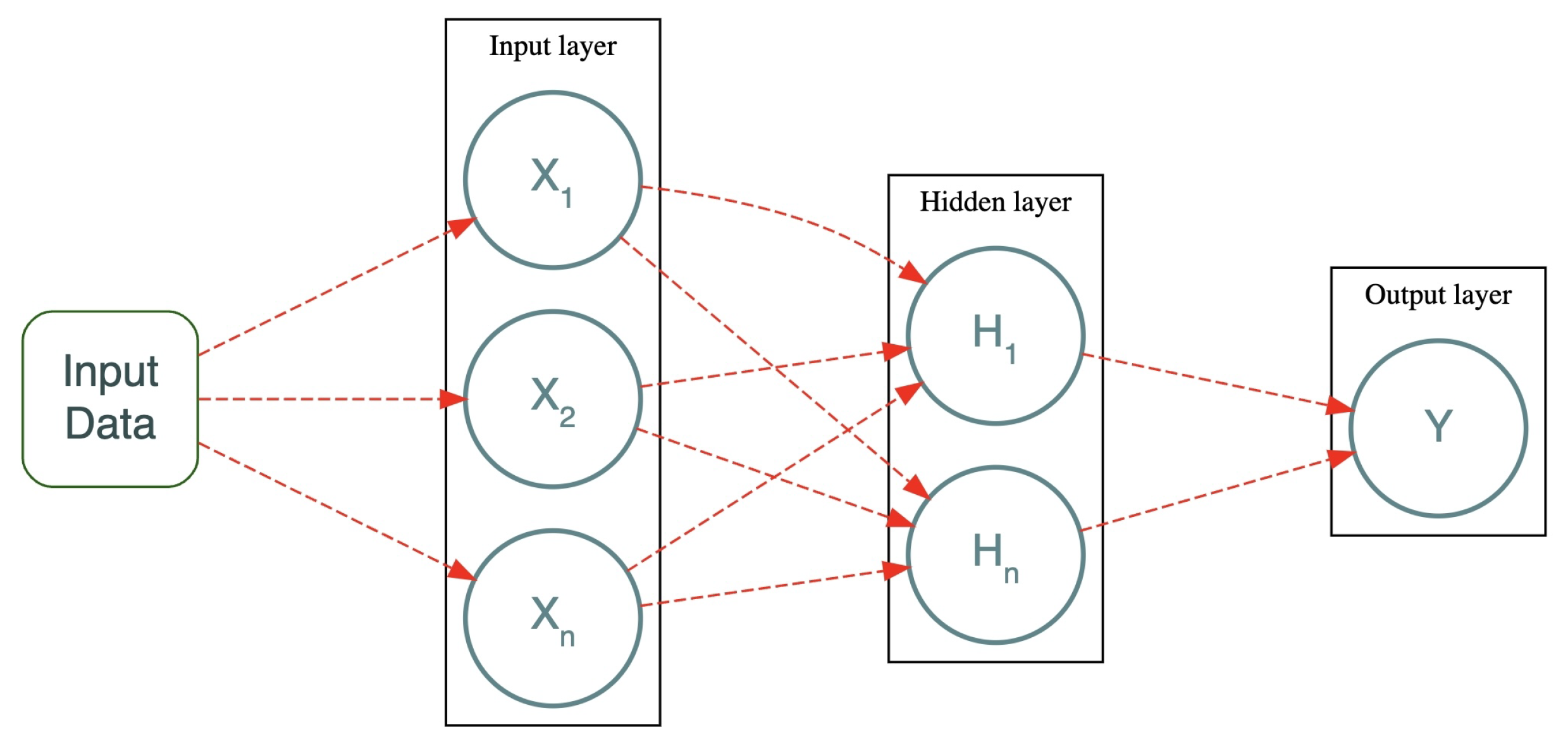
The process of optimal categorization of the image scene into the land categories was performed iteratively using the ML tools defining the key parameters of spectral reflectance. The MultiLayer Perceptron (MLP) algorithms are a class of Artificial Neural Network (ANN) methods. The general methodological scheme for the ANN is presented in Figure 6.
In GRASS GIS, the MLPClassifier is derived from the Scikit-Learn Library of Python and is based on fundamentals of predictive learning [64]. Its performance differs from other classifiers since it uses the principle of the feedforward ANN. For data analysis, ANN uses three layers that are used as structures of network topology in the flow of information for data partition. Pixels of the raster layer present the nodes of the input, hidden, and output layers (see Figure 6), which train the model using supervised learning. The principal approach of this process consists of the connection between each node in one layer to those in the following layer through a certain weight (). The MLPClassifier iteratively evaluates the training data using these connections in weights of pixels. The algorithm changes weights repetitively using estimated error until the output image approaches the expected result and the error is minimized. This sequential operation is formulated in Equation (2):
where is the degree of error in an output node j in the n-th pixel of the raster dataset and is the node weights, which are iteratively adjusted using the minimization of the errors in the classified raster image for the n-th pixel of the raster matrix. Using optimization, each weight is estimated and changed accordingly, as in Equation (3):
where is the result of the previous step of classification, and is the tuning parameter of optimization, which aims at the quick convergence of the weights of pixels during the iterative process of image classification. Hence, the MLPC algorithm is sensitive to feature scaling, which is related to the resolution of the original raster image. The essential approach of this algorithm consists of the random selection of the hidden nodes and analytical determination of the output weights of neural networks [63]. As a result, the MLPClassifier algorithm ensures higher generalization output at a faster learning speed.
Using ML modules of GRASS GIS, the image classification using the MLPC algorithm was implemented using the combination of the modules “r.learn.train” used for extracting training data, supervised machine learning, and cross-validation using the Python package Scikit-Learn, and the module “r.learn.predict” for estimating prediction of pixels’ classification. The technical implementation was performed using the code in Listing 4:
| Listing 4. GRASS GIS code for RF method for supervised image classification. |
 |
3.4.3. Support Vector Machine
The Support Vector Machine (SVM) Classifier uses supervised learning methods [66] and classifies the data into classes using decisions on the largest separation between the classes. Hence, it discriminates the values of the pixels constituting the images and identifies the largest distance to the nearest training sample. When SVC uses training vectors of sample pixels that are located within the margin of classes using the following algorithm approach—, where as two classes and a vector —it aims to find the and so that the assignment of pixels to correct land cover class is true for most samples using Equation (4):
which depends on the definitions of , which should be greater than one for the optimal prediction of the correctly classified pixels on a raster scene, and . The SVC analyzes Digital Numbers (DNs) of pixels on the image to maximize the margins of the classes using iterative analysis. The estimated decision function in a classified matrix of the image consists of cells for a sample of x pixels, as shown in Equation (5):
The result of the classification assigns the predicted classes and the support vectors, which are summarized using attributes of the classification. The effectiveness of the SVM method is that it is a memory-efficient approach that optimizes the use of the computational capacities of the machine. The flexibility of this algorithm is ensured by different Kernel functions defined, which include both common and custom kernels. The practical implementation of this approach in GRASS GIS is presented in Listing 5 below. First, the SVC model is trained using the “r.learn.train” module. Then, the prediction of pixel assignments is carried out using the “r.learn.predict” module. Afterward, the raster categories thatare automatically applied to the classification output are checked using “r.category” module. The visualization is performed using the modules “r.colors”, “d.rast”, and “d.legend”. An example of the code used for classification of the image for 2019 is presented below.
| Listing 5. GRASS GIS code for SVC method for supervised image classification. |
 |
The GitHub repository is created to summarize the methodology and the results of all the models and classification outputs. The programming scripts used for plotting the data, confusion matrices, and maps are also included in this repository for a comparative analysis of the statistical outputs and quantitative estimations on land cover types.
The overall performance of the tested ML classifiers and ANN were evaluated for accuracy, F1 score, Cohen’s kappa coefficient, and other parameters. Here, Cohen’s kappa is a quantitative measure that evaluates the reliability of rating coefficients that assess the accuracy of pixels’s classification and assignment to diverse land cover types [90]. The applicability of Cohen’s Kappa techniques for data evaluation is proven by their use in various studies [91,92,93]. The reliability was evaluated for three classifiers—(1) Random Forest Classifier, (2) Support Vector Machine (SVM) Classifier, and (3) Multilayer Perceptron Classifiers (MLPClassifier)—to evaluate the accuracy of these approaches to satellite image processing. Cohen’s Kappa is an important factor in the interpretation of test findings regarding raster image classification. In this study, Cohen’s kappa was defined in weighted form using the formula in Equation (6):
where the indicates the probability of agreement and is the probability of random agreement. The advantage of Cohen’s kappa is that it presents a robust measure of estimating the statistical probability of evaluation compared to the simple percent agreement calculation [94]. This is possible since Cohen’s kappa takes into account the possibility of the random agreement of pixels’ assignment to diverse land cover classes. Hence, it is an appropriate measure of the reliability of pixels assigned to diverse land cover classes. In this way, Cohen’s kappa estimates the degree to which these classifiers produce similar results under consistent environmental conditions of landscapes, that is, the same date, sunlight, and azimuth angle of the satellite images.
In contrast to Cohen’s Kappa, the F-score evaluates the predictive performance and classification performance. Generally, it is calculated from the precision of the classification using the number of correctly classified pixels divided by the number of all samples that are predicted to be correct. Precision indicates the positive predictive value in sensitive classification [95,96]. According to previous studies on image classification [97], the estimation of the F score is performed using the following formula in Equation (7):
Widely used in diverse cases of image processing, such as classification, partition, or segmentation [98,99,100], the F1 score presents the harmonic mean of the precision and recall of image classification model. These two metrics contribute equally to the estimation, which enables the F1 score metric to correctly indicate the reliability of image classification.
4. Results and Discussion
The identified categories include the following land cover types, defined as classes corresponding to the following land cover patterns: (1) salt water bodies (ocean); (2) brackish water (lake); (3) wetlands and coastal lagoon; (4) dense deciduous forest; (5) agricultural land, croplands; (6) trees and vegetated areas; (7) built-up and urban areas; (8) grassland and shrubland; (9) rural areas; and (10) freshwater (river). The spatio-temporal change in land cover types around Chilika Lake between the years 2019 and 2024 is shown in maps presented in Figure 7, Figure 8, Figure 9 and Figure 10 and compared with existing similar research [35,101]. The hydrological effects can be explained by the increase in water turbidity during the spring period, which affects the visibility of the lake surface through the decreased transparency of the water column affected by the increased photosynthetic activity during this period. The distribution of mangroves that are mostly situated along the tidal water ways are distinguished due to their spectral separability on the EO data. Thus, salt marsh grasses are generally located along the tidal flats due to the specific environmental setting of these physiographic units.
The areas of wetlands and coastal lagoon as well as water bodies increased due to new mouth opening of the Chilika Lake. The scrubland and grassland decreased, while the forest areas increased. This numerical computations of changes are summarized in Table 1, and the statistical report tables are provided in the GitHub repository. The dynamics in land cover types in the coastal area of Chilika imply that that scrubland and grassland were converted into forest due to higher dense vegetation cover. Notably, the agriculture fallow land does not show much difference between the estimated years of 2019 and 2024.
The comparative analysis of the maps shows that the surroundings of the Chilika Lake underwent changes in land cover types. This was caused by the cumulative effects from both the anthropogenic and natural events and results in variations of biological productivity, water eutrophication, and the extent of mangrove forests which strongly depend on the variations in the salinity as discussed above. In turn, the salinity level in the lake is regulated by the monsoon processes and the changes in oceanic seawater and river inflow and counterparts. The effects from the human activities in the watershed of Chilika lagoon result in increased siltation and an increase in nutrients. The land cover types were identified on the satellite images in the study area using information on classification adopted from existing studies [71]; see Figure 7.
During the evaluated period of 2019–2024, notable changes were observed in the Chilika Lake surroundings, including settlements and populated built-up areas, agriculture lands, croplands and plantations, and barren or wasteland areas. At the same time, other classes did not show many differences in the five-year time span. Between 2019 and 2024 (Table 1), the area of agricultural plantations as well as barren land decreased, while urban population areas and built-up areas occupied by settlements increased. The increase in the settlement and built-up areas is identified between 2019 and 2022 and between 2023 and 2024, which might refer to the natural increase in urban population caused by socio-economic drivers; see Figure 8.
Besides the anthropogenic issues, the variations in the color and salinity of water within the Chilika Lake visible on the images are related to the monsoon rains, which strongly influence the hydrography of the coastal lagoon; see Figure 9. Thus, the inflow of sediment and water from the catchments of rivers and tributaries upstream are at a maximum during monsoon months. This is also increased by the oceanic sediment transport. Consequently, these months are notable for intensive floods and turbulence of waters in the coastal lagoon. Accordingly, the impact of both oceanic tides and freshwater inflow from the rivers regulate the salinity of Chilika Lake and change it depending on the dominating force.
Spatial variability of the salinity detected in the images classified using the ANN-based MLPClassifier demonstrates the decrease during the monsoon period due to the influx of freshwater, which especially concerns the northern and central segments of the lake, while the southern sector is the least affected even during monsoon and maintains its brackish-water conditions; see Figure 10. Such hydrological patterns are well reflected in the satellite images, which show various colors of water in the lake. During spring periods, when the images were taken, the water level of the lagoon gradually decreases and reaches its lowest level during summer. Finally, the effects of winds also creates an input into the balance of salinity of the Chilika Lake by water turbidity in upper layers. Such climate effects facilitate the influx of saline water from the ocean and increase the salinity of the lake accordingly. In turn, the variability in salinity and geochemical characteristics related to such complex processes affect aquatic vegetation and algae bloom during favorable periods, which can be identified in the satellite images.
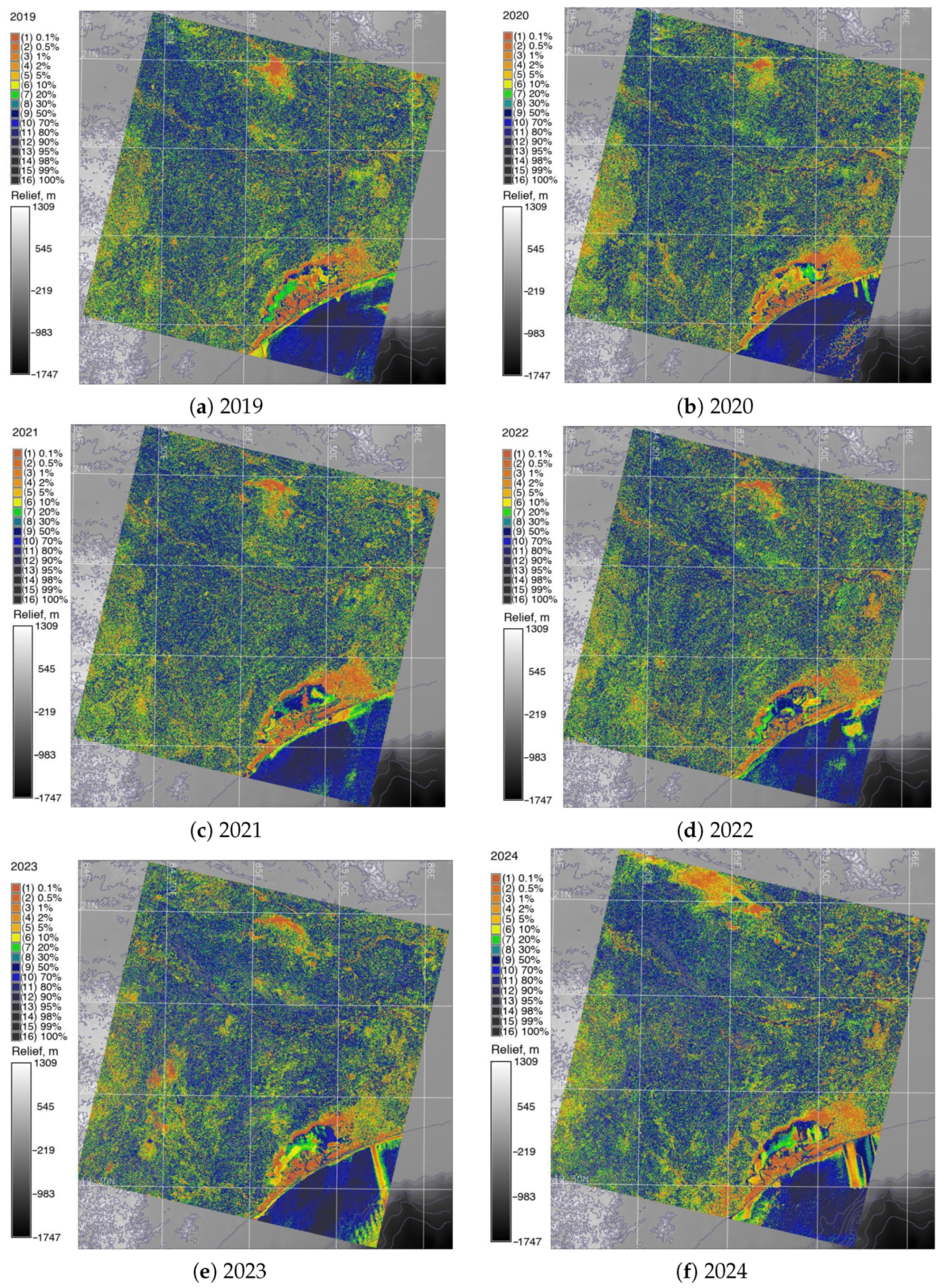
The siltation, increase in nutrient enrichment, and reduced salinity favored the growth of weeds and eutrophication within the basin of lake. Such changes can be detected by computer vision algorithms using the Random Forest method due to different levels of spectral reflectance of the lacustrine surface; see Figure 8. Hence, spring algal bloom in the inland waters of Chilika Lake is a major issue in the spring period, when the imagery was taken, which in turn affects water quality, especially in the shallow estuarine segments of the lake. Furthermore, the effects of eutrophication lead to the degradation of the aquatic habitats. For instance, the level of eutrophication increased in the lake from 2019 to 2020 and 2021, after which the situation stabilised. The results of image classification using SVM method are presented in Figure 9. Image analysis showed that the algal growth is increased in 2021 and 2024, which was best detected using the ANN approach of MLPClassifier, Figure 10. The evaluation of accuracy was performed using chi-square test and visualized in Figure 11.
Accordingly, the stability of points assigned to land cover classes were evaluated and reported as follows for each year: for 2019, 98.08% points stable; for 2020, 98.23%; for 2021, 98.19%; for 2022, 98.25%; for 2023, 98.37%; and for 2024, 98.08% points stable, respectively. Finally, class means and standard deviations computed for each band and each year, respectively, are presented in the Table A2 in Appendix B for the years 2019 to 2024. The maps of accuracy analysis assessment of image classification has been performed using rejection-threshold probability techniques using chi square test, the results of which are presented in Figure 11.
The final results of the computations included the convergence for iterations of pixels assigned to the land cover classes. The convergence was computed for each image and demonstrated the following results: for the year 2019, 98.1%; for the year 2020, 98.2%; for the year 2021, 98.2%; for the year 2022, 98.2%; for the year 2023, 98.4%; and for the year 2024, 98.1%. This shows high precision and accuracy of the calculations using GRASS GIS algorithms of image processing. The class separability matrices computed for 10 land cover types identified in the Chilika lagoon for the years 2019, 2020, 2021, 2022, 2023, and 2024 are reported in the tables placed in Appendix C. The GitHub repository with GRASS GIS scripts and the results of the ANN and ML image processing is available online at https://github.com/paulinelemenkova/India_Chilika_Lake_GRASS_GIS_ANN_ML_Image_Processing (accessed on 4 April 2024) and contains the results of the image processing.
Diverse types of lacustrine vegetation such as weeds and grasses distributed along the sheltered lagoon margins include dense algae meadows on the flats and shallow water areas, which are mostly occupied by brackish weeds and other marsh grasses. Such vegetation largely depends on the specific lacustrine environment and is naturally distributed along the inner margin of the Chilika coasts. Marine influences on the Chilika coastal lagoon are directed through the barrier spits and estuaries of the adjacent rivers. Among the environmental problems that affected the variations in the land cover types are the strong eutrophication, which was visible on the images due to the heavy nutrient upload.
Change-detection analysis in the land cover types from 2013 to 2023 demonstrated shifts in land cover types within the basin of the Chilika Lake coastal lagoon. The computed areas occupied by various land cover classes for each of the category are summarized in Table 1. Such variability of landscape patches around the Chilika Lake proved the existence of fluctuations in the processes of siltation and eutrophication in the coastal lagoon over the studied period (years 2019–2024). Major causes of such environmental changes are related to sedimentation processes such as low river flow speed, which cause stagnation of water and eutrophication. Second, the increased sediment budgetary balance and flushing of sediments into the Bay of Bengal also contribute to the changes in the lake level. Since water fluctuations in various parts of the Chilika Lake are subject to monsoon effects in dry and wet seasons, wetland types can be discriminated on the satellite images along the margin areas of the lagoon. These variations are also caused by the different hydrological effects (e.g., currents and water level) and geomorphic settings of the surrounding relief.
Table 2 compares the hyper parameters of the GRASS GIS used for classification indices in for ANN and various models of ML. Cohen’s Kappa was computed to compare the results of raster image classification, such as landscapes viewed by RS Landsat sensors and identified using ANN and ML algorithms of GRASS GIS. In this way, Cohen’s Kappa presents a straightforward statistical approach that computes the confusion matrix by considering each pixel of the comparable raster images as a single rating made by two raters. In this regard, the results were computed and summarized below.
Table 2 summarizes and compares such parameters as accuracy, F1 score, Cohen’s kappa coefficient, and related parameters. Based on the computed values of Cohen’s Kappa coefficient and the F1 method for the evaluation of classified data, the results suggest that the 0.785 Cohen’s Kappa coefficient and F1 score of 0.89 are rated as the good strength of agreement. Hence, the ANN technique can be interpreted as a reliable approach for satellite image classification in terms of accuracy, followed by the SVM and RF. The interpretation of the F score is as follows. The highest possible value of 1.0 indicates the perfect precision and recall of variables, while the lowest theoretically possible value of 0 indicates the lowest precision or recall which are zero in this case. Hence, higher values generally mean better results of satellite image classification. Likewise, as other correlation statistics, the kappa can range from −1 to +1. The interpretation of values is as follows. Values of the levels of 0.60 to 0.79 have a moderate level of agreement, those in the interval of 0.8–0.9 (that is, over 80% below 90%) are acceptable as having strong level of agreement, and those above 0.9 are almost perfect [102].
The short-term evolution of the physiographic habitats and land cover types around the Chilika coastal lagoon is strongly affected by the humid monsoon climate of the Bay of Bengal and human activities. The analysis of satellite images performed using ML and ANN algorithms enabled us to recognize fluctuations over the areas of Chilika lagoon, which depend on the water level, tidal level, monsoon effects, and inflow of rivers of Daya and Bhargavi into the lagoon. In terms of technical capabilities, the ANN model performed the best in terms of learning capabilities of the model in GRASS GIS and the effectiveness in capturing anomalies and outliers in classified pixels assigned to various land cover classes. Although the ANN model required high computational resources and was demonstrated to be a highly time-consuming model, its performance was excellent with regard to the other models. Furthermore, the lagoon depends on the inflow from the sea waters through the small stream inlets. Such variations in hydrology strongly affect the lacustrine environments, as demonstrated on the satellite images processed using GRASS GIS.
Wetlands, swamps, and mangroves situated along the coasts of the Chilika lagoon are modified by the increase in sediments, which is in turn caused by the effects from monsoon storms and repetitive local floods in the estuaries. Thus, spatial variations in the lake’s surface revealed the topographic differences between various regions of the lagoon. For instance, its western part is more vulnerable to geomorphic erosion due to higher topographic elevations. This is exaggerated by the more intense fishing in this part of the lagoon, which is caused by the location of settlements and villages placed in this region. Finally, high rainfall triggered runoff, which affected the watershed of the Chilika Lake.
High biodiversity in the physiographic setting of the Chilika lagoon affected the structure and intensity of the habitat dynamics in its ecosystems. Thus, the complex mosaic of the vegetation types detected on the multispectral satellite images point at different geomorphic and landscape units of the lagoon system. Local variations in the vegetation distribution along the fringes of the Chilika lagoon are caused by the periodic monsoon effects on the hydrological system and interruptions in the sedimentation process, which depend on the riverine inflow as discussed above. These processes are intensified by local soil erosion, monsoon storms, and fishery activities, which have affected the distribution of vegetation on tidal flats and the surrounding landscapes.
Social and ecological implications of the presented findings include mapping lacustrine landscapes of Chilika Lake in East India for spatio-temporal analysis of changes in land cover types quality and extent. Specifically, the evaluated changes enable the detection of eutrophication and dynamics in the nearby landscapes, which is essential for the environmental monitoring of the coastal lagoons.
5. Conclusions
Mapping coastal lagoons using RS data over time is important for distinguishing the effects of climate and anthropogenic impacts causing major natural disturbances in the surrounding landscapes. This study demonstrated the application of ML/ANN techniques for satellite image processing, aiming to map and visualize changes over the coastal landscape of Chilika Lake in the 2019–2024 time period. The mosaic of ten land cover types was identified around the Chilika Lake and recognized at a resolution of 30 m using GRASS GIS techniques of ML applied to satellite image processing, allowing an assessment of individual landscape patches. Technically, we analyzed the difference between the effects of diverse ML algorithms (Maximal Likelihood discriminant analysis, Random Forest, Support Vector Machine, and MLPClassifier of ANN) on Landsat image analysis and the effects of these approaches on image classification.
Owing to technological limitations of existing GIS tools (traditional methods of classification), some previous mapping efforts in the Chilika Lake relied on a relatively coarse discrimination of land/water coverage and the detection variability of land cover types, including mangroves. These were referred to as potential aquatic habitatsto analyze all coastal areas where land cover changes would likely occur. In contrast, this study revealed the effectiveness of the ML/ANN algorithms for RS data classification, which present a powerful alternative to the traditional cartographic tasks through the automation of image classification.
The results of this research show the impact of climate variability on changes in land cover types during short-term time gap and landscape dynamics around the lagoon of Chilika Lake. Recent boundaries of coastal land categories (2023) closely followed the contour of previous patches detected on earlier images (e.g., 2020, 2019), largely because the extent of the lake limits the existing land cover types, as well as distribution of aquatic vegetation and restrict mangroves to shallow depths with brackish water. The implications of this study are useful for environmental decision-making and can support in policy-making in the sustainable development of Ramsar marine sites of India. The paper also demonstrated the value of EO data for environmental analysis. Landsat 8-9 OLI/TIRS satellite images provide an added value to the conventional environmental analysis through land cover classification using ML methods.
Machine learning (ML) and ANN techniques were evaluated for satellite image processing and proved their effectiveness and usefulness for the environmental analysis performed using GRASS GIS. The use of such data and methods can improve cartographic results in coastal areas that observe some structural variability in landscape patches. A landsat sensor with moderate spectral and high temporal resolution has proven useful in estimating the spatio-temporal variations in land cover types in the coastal lagoon of Chilika Lake in early spring period since 2019 to 2024. Specifically, Random Forest, Support Vector Machine, and MultiLayer Perceptron classifier algorithms were successful in capturing the trend of landscape dynamics in the lacustrine surroundings using ML methods of the automatic analysis of spectral reflectance of pixels. Similarly, the scripting algorithm of GRASS GIS enabled the cartographic workflow using different modules for raster data processing.
Time series maps of land cover types derived from the classified Landsat images explained the overall relationship between climate effects, environmental patterns, and hydrological processes through sedimentation, algal bloom detected in the lake during the spring period, and variations in land cover types of the surrounding landscapes in eastern India, as evaluated during a short-term period of the past six years.
Funding
The APC was funded by the IOAP Participant University of Salzburg.
Institutional Review Board Statement
Not applicable.
Informed Consent Statement
Not applicable.
Data Availability Statement
The open GitHub repository with GRASS GIS scripts and the results of the ANN and ML modelling of the satellite images used for RS data processing are available online at https://github.com/paulinelemenkova/India_Chilika_Lake_GRASS_GIS_ANN_ML_Image_Processing (accessed on 4 April 2024).
Conflicts of Interest
The author declares no conflicts of interest.
Abbreviations
The following abbreviations are used in this manuscript:
| ANN | Artificial Neural Networks |
| CDOM | Coloured Dissolved Organic Matter |
| DL | Deep Learning |
| DN | Digital Number |
| EO | Earth Observation |
| GEBCO | General Bathymetric Chart of the Oceans |
| GMT | Generic Mapping Tools |
| GRASS | Geographic Resources Analysis Support System |
| GIS | Geographic Information System |
| Landsat OLI/TIRS | Landsat Operational Land Imager and Thermal Infrared Sensor |
| ML | Machine Learning |
| MLP | MultiLayer Perceptron |
| RF | Random Forest |
| RS | Remote Sensing |
| SVM | Support Vector Machines |
| USGS | United States Geological Survey |
| UTM | Universal Transverse Mercator |
| WGS84 | World Geodetic System 84 |
| WRS | Worldwide Reference System |
Appendix A. Metadata for the Landsat 8-9 OLI/TIRS images obtained from the USGS

Table A1.
Metadata for the Landsat 8-9 OLI/TIRS images obtained from the USGS.
| Data Set Attribute | Attribute Value | Attribute Value | Attribute Value |
|---|---|---|---|
| Landsat Scene Identifier | LC81400462019044LGN00 | LC81400462020063LGN00 | LC81400462021033LGN00 |
| Date Acquired | 2019/02/13 | 2020/03/03 | 2021/02/02 |
| Roll Angle | 0 | 0 | 0 |
| Start Time | 2019-02-13 04:43:38.496305 | 2020-03-03 04:43:50.54638 | 2021-02-02 04:44:01.299722 |
| Stop Time | 2019-02-13 04:44:10.266304 | 2020-03-03 04:44:22.316379 | 2021-02-02 04:44:33.069722 |
| Land Cloud Cover | 0.01 | 0.01 | 0.01 |
| Scene Cloud Cover L1 | 0.01 | 0.10 | 0.01 |
| Ground Control Points Model | 537 | 568 | 511 |
| Geometric RMSE Model | 6517 | 6132 | 6777 |
| Geometric RMSE Model X | 4631 | 4199 | 4899 |
| Geometric RMSE Model Y | 4586 | 4468 | 4683 |
| Processing Software Version | LPGS_15.3.1c | LPGS_15.3.1c | LPGS_15.4.0 |
| Sun Elevation L0RA | 46.81303022 | 52.31490489 | 44.35249578 |
| Sun Azimuth L0RA | 139.03612161 | 132.76708087 | 142.18104190 |
| TIRS SSM Model | FINAL | FINAL | FINAL |
| Data Type L2 | OLI_TIRS_L2SP | OLI_TIRS_L2SP | OLI_TIRS_L2SP |
| Satellite | 8 | 8 | 8 |
| Scene Center Lat DMS | 20°13′48.04″ N | 20°13′47.89″ N | 20°13′47.39″ N |
| Scene Center Long DMS | 85°06′11.16″ E | 85°05′14.89″ E | 85°05′49.38″ E |
| Corner Upper Left Lat DMS | 21°16′11.10″ N | 21°16′10.16″ N | 21°16′10.70″ N |
| Corner Upper Left Long DMS | 83°58′48.18″ E | 83°57′56.20″ E | 83°58′27.41″ E |
| Corner Upper Right Lat DMS | 21°17′41.71″ N | 21°17′41.46″ N | 21°17′41.60″ N |
| Corner Upper Right Long DMS | 86°11′48.91″ E | 86°10′56.86″ E | 86°11′28.10″ E |
| Corner Lower Left Lat DMS | 19°09′09.76″ N | 19°09′08.93″ N | 19°09′09.43″ N |
| Corner Lower Left Long DMS | 84°01′14.38″ E | 84°00′23.08″ E | 84°00′53.86″ E |
| Corner Lower Right Lat DMS | 19°10′30.65″ N | 19°10′30.43″ N | 19°10′30.54″ N |
| Corner Lower Right Long DMS | 86°12′27.86″ E | 86°11′36.49″ E | 86°12′07.31″ E |
| Landsat Scene Identifier | LC91400462022044LGN01 | LC91400462023063LGN00 | LC81400462024042LGN00 |
| Date Acquired | 2022/02/13 | 2023/03/04 | 2024/02/11 |
| Roll Angle | 0 | 0 | −1 |
| Start Time | 2022-02-13 04:44:06 | 2023-03-04 04:44:07 | 2024-02-11 04:43:59 |
| Stop Time | 2022-02-13 04:44:38 | 2023-03-04 04:44:39 | 2024-02-11 04:44:31 |
| Land Cloud Cover | 0.01 | 0.01 | 1.35 |
| Scene Cloud Cover L1 | 0.01 | 0.01 | 1.24 |
| Ground Control Points Model | 556 | 473 | 454 |
| Geometric RMSE Model | 6320 | 6977 | 6930 |
| Geometric RMSE Model X | 4628 | 4820 | 4746 |
| Geometric RMSE Model Y | 4304 | 5044 | 5049 |
| Processing Software Version | LPGS_16.2.0 | LPGS_16.2.0 | LPGS_16.3.1 |
| Sun Elevation L0RA | 46.93750742 | 52.43682914 | 46.26502602 |
| Sun Azimuth L0RA | 139.05519463 | 132.73529917 | 139.75153012 |
| TIRS SSM Model | N/A | N/A | FINAL |
| Data Type L2 | OLI_TIRS_L2SP | OLI_TIRS_L2SP | OLI_TIRS_L2SP |
| Satellite | 9 | 9 | 8 |
| Scene Center Lat DMS | 20°13′47.24″ N | 20°13′48.14″ N | 20°13′46.99″ N |
| Scene Center Long DMS | 85°04′03.04″ E | 85°03′42.62″ E | 85°02′54.24″ E |
| Corner Upper Left Lat DMS | 21°16′08.83″ N | 21°16′08.47″ N | 21°16′07.54″ N |
| Corner Upper Left Long DMS | 83°56′43.44″ E | 83°56′22.63″ E | 83°55′30.65″ E |
| Corner Upper Right Lat DMS | 21°17′41.10″ N | 21°17′40.99″ N | 21°17′40.74″ N |
| Corner Upper Right Long DMS | 86°09′43.99″ E | 86°09′23.15″ E | 86°08′31.09″ E |
| Corner Lower Left Lat DMS | 19°09′07.78″ N | 19°09′07.42″ N | 19°09′06.59″ N |
| Corner Lower Left Long DMS | 83°59′11.29″ E | 83°58′50.77″ E | 83°57′59.51″ E |
| Corner Lower Right Lat DMS | 19°10′30.11″ N | 19°10′30″ N | 19°10′29.78″ N |
| Corner Lower Right Long DMS | 86°10′24.60″ E | 86°10′04.04″ E | 86°09′12.71″ E |
Appendix B. Class-Separability Matrices for Land Cover Classes
Appendix B.1. Class-Separability Matrices: 2019 and 2020
Appendix B.2. Class-Separability Matrices: 2021 and 2022
Appendix B.3. Class-Separability Matrices: 2023 and 2024
Appendix C. Computed Class Means for Land Cover Classes
Table A2.
Class means of Digital Numbers (DNs) of pixels computed for pixels assigned to 10 land cover classes in the landscapes around Chilika Lake within each Landsat 8-9 OLI/TIRS band (1 to 7) for the years 2019 to 2024.
Table A2.
Class means of Digital Numbers (DNs) of pixels computed for pixels assigned to 10 land cover classes in the landscapes around Chilika Lake within each Landsat 8-9 OLI/TIRS band (1 to 7) for the years 2019 to 2024.
| Class | Band 1 | Band 2 | Band 3 | Band 4 | Band 5 | Band 6 | Band 7 |
|---|---|---|---|---|---|---|---|
| 2019 | |||||||
| 1 | 7384.59 | 7627.99 | 7895.94 | 7432.46 | 7311.54 | 7522.6 | 7534.26 |
| 2 | 8643.32 | 9065.21 | 10,097.8 | 9576.69 | 8982.72 | 8163.85 | 7900.08 |
| 3 | 7909.62 | 8189.18 | 9032.65 | 8872.02 | 13,230.6 | 11,239.2 | 9522.02 |
| 4 | 7855.42 | 8099.7 | 9003.44 | 8780.11 | 15,341.4 | 12,452.6 | 9902.94 |
| 5 | 7993.15 | 8247.89 | 9267.59 | 9042.79 | 16,989.7 | 13,587.9 | 10,478.3 |
| 6 | 8356.75 | 8702.28 | 9805.76 | 9943.78 | 16,308 | 15,025.3 | 11,968.9 |
| 7 | 8386.91 | 8760.24 | 9764.89 | 10,023.5 | 14,226.4 | 14,156.7 | 11,883.2 |
| 8 | 8770.28 | 9187.13 | 10,314.4 | 10,890.7 | 15,345.3 | 16,391.3 | 13,700.7 |
| 9 | 9215.28 | 9707.92 | 10,991.3 | 11,942.4 | 16,298 | 18,419.5 | 15,557.1 |
| 10 | 10,984.1 | 11,566.3 | 13,775 | 15,936.7 | 18,901.8 | 22,878.1 | 21,892.5 |
| 2020 | |||||||
| 1 | 7362.63 | 7605.24 | 8058.61 | 7428.78 | 7302.72 | 7611.18 | 7600.81 |
| 2 | 8799.63 | 9212.01 | 10,298.1 | 9846.45 | 9447.31 | 8374.1 | 8010.46 |
| 3 | 7943.86 | 8190.79 | 9124.49 | 8775.28 | 13,978.1 | 11,732.6 | 9604.04 |
| 4 | 7951.76 | 8182.82 | 9148.86 | 8762.19 | 15,483.8 | 12,974.3 | 10,132.6 |
| 5 | 8046.6 | 8290.53 | 9367.25 | 8877.5 | 17,339.2 | 13,624.9 | 10,362.4 |
| 6 | 8289.78 | 8579.24 | 9693.26 | 9484.22 | 16,220.4 | 14,673.9 | 11,489.4 |
| 7 | 8460.6 | 8784.33 | 9843.28 | 9877.32 | 14,561 | 14,590 | 12,004.6 |
| 8 | 8682.86 | 9047.62 | 10,243.8 | 10,406.1 | 15,846.7 | 16,209.3 | 13,175.8 |
| 9 | 9103.29 | 9524.9 | 10,833.7 | 11,361.1 | 16,366.5 | 18,052.3 | 15,014.9 |
| 10 | 11,001.5 | 11,588.6 | 13,781.4 | 15,754.9 | 19,292 | 23,392.5 | 21,832.9 |
| 2021 | |||||||
| 1 | 7313.11 | 7667.41 | 8116.02 | 7492.57 | 7333.71 | 7574.41 | 7569.82 |
| 2 | 8559.44 | 9073.05 | 10,170.7 | 9669.56 | 8743.74 | 8092.44 | 7874.43 |
| 3 | 7890.09 | 8128.26 | 8880.14 | 8688.48 | 13,228.5 | 11,313.2 | 9513.12 |
| 4 | 7937.49 | 8150.84 | 8974.22 | 8708.31 | 15,426.7 | 12,674.9 | 10,038.2 |
| 5 | 8177.43 | 8412.77 | 9402.44 | 9144.78 | 17,531.1 | 14,258 | 10,941.5 |
| 6 | 8323.64 | 8323.64 | 9565.02 | 9675.27 | 15,282.8 | 14,491.2 | 11,722 |
| 7 | 8517.84 | 8925.77 | 9920.3 | 10,269.8 | 13,560.5 | 14,131.2 | 12,233 |
| 8 | 8759.76 | 9162.3 | 10,257 | 10,789.3 | 15,470.1 | 16,325.2 | 13,607.4 |
| 9 | 9185.24 | 9675.96 | 10,914.1 | 11,894.1 | 16,279 | 18,494.3 | 15,564 |
| 10 | 10,665.1 | 11,305.1 | 13,359.4 | 15,356.5 | 18,762.9 | 22,569.6 | 21,150.5 |
| 2022 | |||||||
| 1 | 7287.88 | 7542.4 | 7718.15 | 7333.43 | 7328.27 | 7592.25 | 7602.72 |
| 2 | 8393.71 | 8875.65 | 10,056.4 | 9608.75 | 8587.92 | 7874.1 | 7714.56 |
| 3 | 7980.49 | 8174.29 | 8866.31 | 8668.13 | 12,794.7 | 10,899 | 9330.4 |
| 4 | 7894.2 | 8035.98 | 8749.86 | 8407.39 | 15,201.5 | 12,022.1 | 9583.49 |
| 5 | 8043.54 | 8188.44 | 8998.54 | 8642.16 | 16,500.8 | 13,086.8 | 10,175.2 |
| 6 | 8239.34 | 8394.65 | 9357.1 | 8940.95 | 18,166.3 | 14,180.8 | 10,795.1 |
| 7 | 8373.31 | 8653.25 | 9575.82 | 9666.31 | 14,750 | 14,098.9 | 11,638.9 |
| 8 | 8681.73 | 9012.21 | 10,079 | 10,388.4 | 15,793.3 | 15,933.3 | 13,111 |
| 9 | 9087.7 | 9499.76 | 10,744.1 | 11,422.2 | 16,621.3 | 17,967 | 14,981.3 |
| 10 | 11,402 | 12,007.2 | 14,459.4 | 16,913.6 | 20,170.8 | 24,147.3 | 23,184.8 |
| 2023 | |||||||
| 1 | 7304.03 | 7602.46 | 7970.98 | 7495.23 | 7370.22 | 7582.83 | 7594.02 |
| 2 | 8642.8 | 9116.27 | 10,225.1 | 9774.06 | 9373.03 | 8426.53 | 8095.8 |
| 3 | 8014.89 | 8370.33 | 9293.49 | 9184.49 | 13,666.4 | 12,570.5 | 10,418.6 |
| 4 | 7968.43 | 8317.51 | 9403.97 | 9059.22 | 16,418 | 13,040.4 | 10,214.3 |
| 5 | 8206.12 | 8585.66 | 9631.98 | 9656.67 | 15,258.8 | 14,373 | 11,402.8 |
| 6 | 8608.63 | 9043.92 | 9991.65 | 10,366.6 | 13,513.2 | 14,643.5 | 12,720 |
| 7 | 8548.43 | 8996.5 | 10,126.3 | 10,475.4 | 15,733.1 | 15,917.6 | 12,836.8 |
| 8 | 8930.24 | 9432.99 | 10,581.5 | 11,287.2 | 15,432.7 | 17,203 | 14,389.8 |
| 9 | 9276.42 | 9835.91 | 11,120.3 | 12,167.4 | 16,591.8 | 19,125.6 | 15,989.6 |
| 10 | 10,626.8 | 11,262.9 | 13,202.7 | 15,146.2 | 18,487.7 | 22,653.8 | 21,910.9 |
| 2024 | |||||||
| 1 | 7381.12 | 7610.35 | 8182.73 | 7489.11 | 7376.46 | 7674.92 | 7641.93 |
| 2 | 8848.7 | 9278.52 | 10,342.7 | 9654.98 | 9050.44 | 8198.38 | 7879.74 |
| 3 | 7962.57 | 8225.6 | 9233.13 | 8808.4 | 13,449.8 | 11,533.5 | 9636.85 |
| 4 | 7885.21 | 8122.14 | 9193.83 | 8670.85 | 15,442.6 | 12,508.1 | 9847.4 |
| 5 | 8119.25 | 8419.77 | 9677.19 | 9141.91 | 17,614 | 14,001.8 | 10,667.5 |
| 6 | 8197.23 | 8499.11 | 9635.42 | 9360.85 | 15,391.6 | 14,031.7 | 11,128.3 |
| 7 | 8467.78 | 8852.79 | 10,008.4 | 10,005.2 | 13,939.7 | 14,177.3 | 11,928.9 |
| 8 | 8602.61 | 9007.3 | 10,280.5 | 10,373.2 | 15,568 | 15,923.8 | 12,996.3 |
| 9 | 9060 | 9554.25 | 10,903.5 | 11,426.4 | 16,024.9 | 17,919.3 | 14,963.6 |
| 10 | 11,029.6 | 11,776.7 | 14,159 | 16,012.6 | 19,470.8 | 23,328.6 | 21,960.9 |
References
- Amaral, V.; Santos-Echeandía, J.; Ortega, T.; Álvarez Salgado, X.; Forja, J. Dissolved organic matter distribution in the water column and sediment pore water in a highly anthropized coastal lagoon (Mar Menor, Spain): Characteristics, sources, and benthic fluxes. Sci. Total Environ. 2023, 896, 165264. [Google Scholar] [CrossRef] [PubMed]
- Xue, B.; Wang, Z.; Wu, P.; Lu, Y.; Diao, M. Effects of geomorphic-induced turbulence on horizontal mixing in the coastal lagoon Xiaohai in China. Reg. Stud. Mar. Sci. 2023, 64, 103048. [Google Scholar] [CrossRef]
- Mao, M.; Xia, M. Seasonal dynamics of water circulation and exchange flows in a shallow lagoon-inlet-coastal ocean system. Ocean. Model. 2023, 186, 102276. [Google Scholar] [CrossRef]
- Cebrian, J.; Corcoran, A.A.; Stutes, A.L.; Stutes, J.P.; Pennock, J.R. Effects of ultraviolet-B radiation and nutrient enrichment on the productivity of benthic microalgae in shallow coastal lagoons of the North Central Gulf of Mexico. J. Exp. Mar. Biol. Ecol. 2009, 372, 9–21. [Google Scholar] [CrossRef]
- Mateos-Molina, D.; Bejarano, I.; Pittman, S.J.; Möller, M.; Antonopoulou, M.; Jabado, R.W. Coastal lagoons in the United Arab Emirates serve as critical habitats for globally threatened marine megafauna. Mar. Pollut. Bull. 2024, 200, 116117. [Google Scholar] [CrossRef] [PubMed]
- Zamora-López, A.; Guerrero-Gómez, A.; Torralva, M.; Zamora-Marín, J.M.; Guillén-Beltrán, A.; Oliva-Paterna, F.J. Shallow waters as critical habitats for fish assemblages under eutrophication-mediated events in a coastal lagoon. Estuar. Coast. Shelf Sci. 2023, 291, 108447. [Google Scholar] [CrossRef]
- Mignucci, A.; Forget, F.; Villeneuve, R.; Derridj, O.; McKindsey, C.W.; McKenzie, D.J.; Bourjea, J. Residency, home range and inter-annual fidelity of three coastal fish species in a Mediterranean coastal lagoon. Estuar. Coast. Shelf Sci. 2023, 292, 108450. [Google Scholar] [CrossRef]
- Pérez-Ruzafa, A.; Pérez-Ruzafa, I.M.; Newton, A.; Marcos, C. Chapter 15—Coastal Lagoons: Environmental Variability, Ecosystem Complexity, and Goods and Services Uniformity. In Coasts and Estuaries; Wolanski, E., Day, J.W., Elliott, M., Ramachandran, R., Eds.; Elsevier: Amsterdam, The Netherlands, 2019; pp. 253–276. [Google Scholar] [CrossRef]
- Kjerfve, B. Comparative Oceanography of Coastal Lagoons. In Estuarine Variability; Wolfe, D.A., Ed.; Academic Press: Cambridge, MA, USA, 1986; pp. 63–81. [Google Scholar] [CrossRef]
- Boyd, R.; Dalrymple, R.; Zaitlin, B. Classification of clastic coastal depositional environments. Sediment. Geol. 1992, 80, 139–150. [Google Scholar] [CrossRef]
- Danish, M.; Tripathy, G.R.; Rahaman, W. Submarine groundwater discharge to a tropical coastal lagoon (Chilika lagoon, India): An estimation using Sr isotopes. Mar. Chem. 2020, 224, 103816. [Google Scholar] [CrossRef]
- Kumar, A.; Equeenuddin, S.M.; Mishra, D.R.; Acharya, B.C. Remote monitoring of sediment dynamics in a coastal lagoon: Long-term spatio-temporal variability of suspended sediment in Chilika. Estuar. Coast. Shelf Sci. 2016, 170, 155–172. [Google Scholar] [CrossRef]
- Bortolin, E.; Weschenfelder, J.; Fernandes, E.; Bitencourt, L.; Möller, O.; García-Rodríguez, F.; Toldo, E. Reviewing sedimentological and hydrodynamic data of large shallow coastal lagoons for defining mud depocenters as environmental monitoring sites. Sediment. Geol. 2020, 410, 105782. [Google Scholar] [CrossRef]
- Larson, M. Coastal Lagoons. In Encyclopedia of Lakes and Reservoirs; Springer: Dordrecht, The Netherlands, 2012; pp. 171–174. [Google Scholar] [CrossRef]
- Pérez-Ruzafa, A.; Molina-Cuberos, G.J.; García-Oliva, M.; Umgiesser, G.; Marcos, C. Why coastal lagoons are so productive? Physical bases of fishing productivity in coastal lagoons. Sci. Total Environ. 2024, 922, 171264. [Google Scholar] [CrossRef] [PubMed]
- Kennish, M.J. Coastal Lagoons. In Encyclopedia of Estuaries; Springer: Dordrecht, The Netherlands, 2016; pp. 140–143. [Google Scholar] [CrossRef]
- Bastos, M.; Roebeling, P.; Alves, F.; Villasante, S.; Magalhães Filho, L. High risk water pollution hazards affecting Aveiro coastal lagoon (Portugal) – A habitat risk assessment using InVEST. Ecol. Inform. 2023, 76, 102144. [Google Scholar] [CrossRef]
- Suwandhahannadi, W.; Le De, L.; Wickramasinghe, D.; Dahanayaka, D. Community participation for assessing and managing ecosystem services of coastal lagoons: A case of the Rekawa Lagoon in Sri Lanka. Ocean. Coast. Manag. 2024, 251, 107069. [Google Scholar] [CrossRef]
- Mohapatra, M.; Manu, S.; Kim, J.Y.; Rastogi, G. Distinct community assembly processes and habitat specialization driving the biogeographic patterns of abundant and rare bacterioplankton in a brackish coastal lagoon. Sci. Total Environ. 2023, 879, 163109. [Google Scholar] [CrossRef] [PubMed]
- Simantiris, N.; Avlonitis, M. Effects of future climate conditions on the zooplankton of a Mediterranean coastal lagoon. Estuar. Coast. Shelf Sci. 2023, 282, 108231. [Google Scholar] [CrossRef]
- Ghandourah, M.A.; Orif, M.I.; Al-Farawati, R.K.; El-Shahawi, M.S.; Abu-Zeid, R.H. Illegal pollution loading accelerate the oxygen deficiency along the coastal lagoons of eastern Red Sea. Reg. Stud. Mar. Sci. 2023, 63, 102982. [Google Scholar] [CrossRef]
- Davis, R.A., Jr.; FitzGerald, D. Coastal Lagoons. In Beaches and Coasts; John Wiley & Sons, Ltd.: Hoboken, NJ, USA, 2019; Chapter 10; pp. 229–245. [Google Scholar] [CrossRef]
- Kumari, A.; Harshawardhan, R.; Kushawaha, J.; Nandi, I. Spatial Identification of Vulnerable Coastal Ecosystems for Emerging Pollutants. In Coastal Ecosystems: Environmental Importance, Current Challenges and Conservation Measures; Springer International Publishing: Cham, Switzerland, 2022; pp. 359–386. [Google Scholar] [CrossRef]
- Herbert, R.J.; Ross, K.; Whetter, T.; Bone, J. Chapter 32—Maintaining ecological resilience on a regional scale: Coastal saline lagoons in a northern European marine protected area. In Marine Protected Areas; Humphreys, J., Clark, R.W., Eds.; Elsevier: Amsterdam, The Netherlands, 2020; pp. 631–647. [Google Scholar] [CrossRef]
- Garcés-Ordóñez, O.; Saldarriaga-Vélez, J.F.; Espinosa-Díaz, L.F.; Canals, M.; Sánchez-Vidal, A.; Thiel, M. A systematic review on microplastic pollution in water, sediments, and organisms from 50 coastal lagoons across the globe. Environ. Pollut. 2022, 315, 120366. [Google Scholar] [CrossRef]
- Bruschi, R.; Pastorino, P.; Barceló, D.; Renzi, M. Microplastic levels and sentinel species used to monitor the environmental quality of lagoons: A state of the art in Italy. Ecol. Indic. 2023, 154, 110596. [Google Scholar] [CrossRef]
- Tripathi, P.; Singhal, A.; Jha, P.K. Metal Transport and Its Impact on Coastal Ecosystem. In Coastal Ecosystems: Environmental Importance, Current Challenges and Conservation Measures; Springer International Publishing: Cham, Switzerland, 2022; pp. 239–264. [Google Scholar] [CrossRef]
- Carrasco, A.; Ferreira, O.; Roelvink, D. Coastal lagoons and rising sea level: A review. Earth Sci. Rev. 2016, 154, 356–368. [Google Scholar] [CrossRef]
- Inácio, M.; Barboza, F.; Villoslada, M. The protection of coastal lagoons as a nature-based solution to mitigate coastal floods. Curr. Opin. Environ. Sci. Health 2023, 34, 100491. [Google Scholar] [CrossRef]
- Lunardini, F.; Di Cola, G. Oxygen dynamics in coastal and lagoon ecosystems. Math. Comput. Model. 2000, 31, 135–141. [Google Scholar] [CrossRef]
- Lugliè, A.; Pulina, S.; Bruno, M.; Mario Padedda, B.; Teodora Satta, C.; Sechi, N. Marine toxins and climate change: The case of PSP from cyanobacteria in coastal lagoons. In Phycotoxins; John Wiley & Sons, Ltd.: Hoboken, NJ, USA, 2015; Chapter 11; pp. 239–253. [Google Scholar] [CrossRef]
- Pauly, D.; Yáñez-Arancibia, A. Chapter 13 Fisheries In Coastal Lagoons. In Coastal Lagoon Processes; Kjerfve, B., Ed.; Elsevier Oceanography Series; Elsevier: Amsterdam, The Netherlands, 1994; Volume 60, pp. 377–399. [Google Scholar] [CrossRef]
- Pedregosa, F.; Varoquaux, G.; Gramfort, A.; Michel, V.; Thirion, B.; Grisel, O.; Blondel, M.; Prettenhofer, P.; Weiss, R.; Dubourg, V.; et al. Scikit-learn: Machine Learning in Python. J. Mach. Learn. Res. 2011, 12, 2825–2830. [Google Scholar]
- GRASS Development Team. Geographic Resources Analysis Support System (GRASS GIS) Software, Version 8.2; Open Source Geospatial Foundation: Beaverton, OR, USA, 2022. [Google Scholar]
- Sinha, R.; Chandrasekaran, R.; Awasthi, N. Geomorphology, Land Use/Land Cover and Sedimentary Environments of the Chilika Basin. In Ecology, Conservation, and Restoration of Chilika Lagoon, India; Springer International Publishing: Cham, Switzerland, 2020; pp. 231–250. [Google Scholar] [CrossRef]
- Barik, S.K.; Bramha, S.; Behera, D.; Bastia, T.K.; Cooper, G.; Rath, P. Ecological health assessment of a coastal ecosystem: Case study of the largest brackish water lagoon of Asia. Mar. Pollut. Bull. 2019, 138, 352–363. [Google Scholar] [CrossRef] [PubMed]
- Mishra, M.; Acharyya, T.; Chand, P.; Santos, C.A.G.; da Silva, R.M.; dos Santos, C.A.C.; Pradhan, S.; Kar, D. Response of long- to short-term tidal inlet morphodynamics on the ecological ramification of Chilika lake, the tropical Ramsar wetland in India. Sci. Total Environ. 2022, 807, 150769. [Google Scholar] [CrossRef] [PubMed]
- Baral, R.; Mohanty, P.K.; Pradhan, S.; Rajawat, A.S.; Samal, R.N.; Das, U. Natural opening of a new inlet in Chilika Lagoon: A cause and impact analysis. Reg. Stud. Mar. Sci. 2023, 68, 103248. [Google Scholar] [CrossRef]
- Cuartero, A.; Paoletti, M.E.; García-Rodríguez, P.; Haut, J.M. PyCircularStats: A Python-Based Tool for Remote Sensing Circular Statistics and Graphical Analysis. In Proceedings of the IGARSS 2022—2022 IEEE International Geoscience and Remote Sensing Symposium, Kuala Lumpur, Malaysia, 17–22 July 2022; pp. 2876–2879. [Google Scholar] [CrossRef]
- Lemenkova, P.; Debeir, O. R Libraries for Remote Sensing Data Classification by k-means Clustering and NDVI Computation in Congo River Basin, DRC. Appl. Sci. 2022, 12, 12554. [Google Scholar] [CrossRef]
- Zhang, M.; Yue, P.; Guo, X. GIScript: Towards an interoperable geospatial scripting language for GIS programming. In Proceedings of the 2014 The Third International Conference on Agro-Geoinformatics, Beijing, China, 11–14 August 2014; pp. 1–5. [Google Scholar] [CrossRef]
- Işik, M.S.; Özbey, V.; Erol, S.; Tari, E. GNSSpy: Python Toolkit for GNSS Data. In Proceedings of the 2021 IEEE International Geoscience and Remote Sensing Symposium IGARSS, Brussels, Belgium, 11–16 July 2021; pp. 8550–8553. [Google Scholar] [CrossRef]
- Lemenkova, P.; Debeir, O. Satellite Image Processing by Python and R Using Landsat 9 OLI/TIRS and SRTM DEM Data on Côte d’Ivoire, West Africa. J. Imaging 2022, 8, 317. [Google Scholar] [CrossRef]
- Erdem, F.; Bayram, B.; Bakirman, T.; Bayrak, O.C.; Akpinar, B. An ensemble deep learning based shoreline segmentation approach (WaterNet) from Landsat 8 OLI images. Adv. Space Res. 2021, 67, 964–974. [Google Scholar] [CrossRef]
- Lemenkova, P.; Debeir, O. Computing Vegetation Indices from the Satellite Images Using GRASS GIS Scripts for Monitoring Mangrove Forests in the Coastal Landscapes of Niger Delta, Nigeria. J. Mar. Sci. Eng. 2023, 11, 871. [Google Scholar] [CrossRef]
- Han, W.; Zhang, X.; Wang, Y.; Wang, L.; Huang, X.; Li, J.; Wang, S.; Chen, W.; Li, X.; Feng, R.; et al. A survey of machine learning and deep learning in remote sensing of geological environment: Challenges, advances, and opportunities. Isprs J. Photogramm. Remote Sens. 2023, 202, 87–113. [Google Scholar] [CrossRef]
- Tarek, M.; Sadek, T.; Hayet, G. Flood-Prone Urban Area Mapping Using Machine Learning, a Case Study of M’sila City (Algeria). In Proceedings of the 2023 International Conference on Earth Observation and Geo-Spatial Information (ICEOGI), Algiers, Algeria, 22–24 May 2023; pp. 1–4. [Google Scholar] [CrossRef]
- Ho, T.K.; Basu, M. Complexity measures of supervised classification problems. IEEE Trans. Pattern Anal. Mach. Intell. 2002, 24, 289–300. [Google Scholar] [CrossRef]
- Wu, L.; Liu, R.; Ju, N.; Zhang, A.; Gou, J.; He, G.; Lei, Y. Landslide mapping based on a hybrid CNN-transformer network and deep transfer learning using remote sensing images with topographic and spectral features. Int. J. Appl. Earth Obs. Geoinf. 2024, 126, 103612. [Google Scholar] [CrossRef]
- G, V.; Goswami, S.; Samal, R.; Choudhury, S. Monitoring of Chilika Lake mouth dynamics and quantifying rate of shoreline change using 30 m multi-temporal Landsat data. Data Brief 2019, 22, 595–600. [Google Scholar] [CrossRef] [PubMed]
- Mishra, M.; Chand, P.; Beja, S.K.; Santos, C.A.G.; da Silva, R.M.; Ahmed, I.; Kamal, A.H.M. Quantitative assessment of present and the future potential threat of coastal erosion along the Odisha coast using geospatial tools and statistical techniques. Sci. Total Environ. 2023, 875, 162488. [Google Scholar] [CrossRef] [PubMed]
- Reddy, C.S.; Khuroo, A.A.; Krishna, P.H.; Saranya, K.; Jha, C.; Dadhwal, V. Threat evaluation for biodiversity conservation of forest ecosystems using geospatial techniques: A case study of Odisha, India. Ecol. Eng. 2014, 69, 287–303. [Google Scholar] [CrossRef]
- Hazra, S.; Ghosh, A.; Ghosh, S.; Pal, I.; Ghosh, T. Assessing coastal vulnerability and governance in Mahanadi Delta, Odisha, India. Prog. Disaster Sci. 2022, 14, 100223. [Google Scholar] [CrossRef]
- Zhao, J.; Wang, Y.; Zhang, H. Automated batch processing of mass remote sensing and geospatial data to meet the needs of end users. In Proceedings of the 2011 IEEE International Geoscience and Remote Sensing Symposium, Vancouver, BC, Canada, 24–29 July 2011; pp. 3464–3467. [Google Scholar] [CrossRef]
- Barma, S.; Damarla, S.; Tiwari, S.K. Semi-Automated Technique for Vegetation Analysis in Sentinel-2 Multi-Spectral remote sensing images using Python. In Proceedings of the 2020 4th International Conference on Electronics, Communication and Aerospace Technology (ICECA), Coimbatore, India, 5–7 November 2020; pp. 946–953. [Google Scholar] [CrossRef]
- Abdali, E.; Valadan Zoej, M.J.; Taheri Dehkordi, A.; Ghaderpour, E. A Parallel-Cascaded Ensemble of Machine Learning Models for Crop Type Classification in Google Earth Engine Using Multi-Temporal Sentinel-1/2 and Landsat-8/9 Remote Sensing Data. Remote Sens. 2024, 16, 127. [Google Scholar] [CrossRef]
- Lukas, P.; Melesse, A.M.; Kenea, T.T. Prediction of Future Land Use/Land Cover Changes Using a Coupled CA-ANN Model in the Upper Omo-Gibe River Basin, Ethiopia. Remote Sens. 2023, 15, 1148. [Google Scholar] [CrossRef]
- Amani, S.; Shafizadeh-Moghadam, H. A review of machine learning models and influential factors for estimating evapotranspiration using remote sensing and ground-based data. Agric. Water Manag. 2023, 284, 108324. [Google Scholar] [CrossRef]
- Li, F.; Yigitcanlar, T.; Nepal, M.; Nguyen, K.; Dur, F. Machine learning and remote sensing integration for leveraging urban sustainability: A review and framework. Sustain. Cities Soc. 2023, 96, 104653. [Google Scholar] [CrossRef]
- Lemenkova, P. Sentinel-2 for High Resolution Mapping of Slope-Based Vegetation Indices Using Machine Learning by SAGA GIS. Transylv. Rev. Syst. Ecol. Res. 2020, 22, 17–34. [Google Scholar] [CrossRef]
- Tselka, I.; Detsikas, S.E.; Petropoulos, G.P.; Demertzi, I.I. Chapter 7—Google Earth Engine and machine learning classifiers for obtaining burnt area cartography: A case study from a Mediterranean setting. In Geoinformatics for Geosciences; Stathopoulos, N., Tsatsaris, A., Kalogeropoulos, K., Eds.; Earth Observation, Elsevier: Amsterdam, The Netherlands, 2023; pp. 131–148. [Google Scholar] [CrossRef]
- Latif, S.D.; Alyaa Binti Hazrin, N.; Hoon Koo, C.; Lin Ng, J.; Chaplot, B.; Feng Huang, Y.; El-Shafie, A.; Najah Ahmed, A. Assessing rainfall prediction models: Exploring the advantages of machine learning and remote sensing approaches. Alex. Eng. J. 2023, 82, 16–25. [Google Scholar] [CrossRef]
- Huang, G.B.; Zhu, Q.Y.; Siew, C.K. Extreme learning machine: Theory and applications. Neurocomputing 2006, 70, 489–501. [Google Scholar] [CrossRef]
- Rosenblatt, F. The perceptron: A probabilistic model for information storage and organization in the brain. Psychol. Rev. 1958, 65, 386–408. [Google Scholar] [CrossRef] [PubMed]
- Ho, T.K. Random decision forests. In Proceedings of the 3rd International Conference on Document Analysis and Recognition, Montreal, QC, Canada, 14–16 August 1995; Volume 1, pp. 278–282. [Google Scholar] [CrossRef]
- Cortes, C.; Vapnik, V. Support-vector networks. Mach. Learn. 1995, 20, 273–297. [Google Scholar] [CrossRef]
- Zhang, H. The Optimality of Naive Bayes. In Proceedings of the Seventeenth International Florida Artificial Intelligence Research Society Conference (FLAIRS 2004); AAAI Press: Menlo Park, CA, USA, 2004; pp. 1–6. [Google Scholar]
- Panda, U.; Mohanty, P.; Samal, R. Impact of tidal inlet and its geomorphological changes on lagoon environment: A numerical model study. Estuar. Coast. Shelf Sci. 2013, 116, 29–40. [Google Scholar] [CrossRef]
- Behera, P.R.; Parida, P.K.; Karna, S.K.; Raman, R.K.; Suresh, V.; Behera, B.K.; Das, B.K. Trophic fingerprinting of Chilika, a Ramsar site and the largest lagoon of Asia using Ecopath. Reg. Stud. Mar. Sci. 2020, 37, 101328. [Google Scholar] [CrossRef]
- Barik, S.K.; Muduli, P.R.; Mohanty, B.; Behera, A.T.; Mallick, S.; Das, A.; Samal, R.; Rastogi, G.; Pattnaik, A.K. Spatio-temporal variability and the impact of Phailin on water quality of Chilika lagoon. Cont. Shelf Res. 2017, 136, 39–56. [Google Scholar] [CrossRef]
- Behera, D.K.; Jamal, S.; Ahmad, W.S.; Taqi, M.; Kumar, R. Estimation of Soil Erosion Using RUSLE Model and GIS Tools: A Study of Chilika Lake, Odisha. J. Geol. Soc. India 2023, 99, 406–414. [Google Scholar] [CrossRef]
- Nazneen, S.; Mahmood, G.; Jafar, Z.; Madhav, S. Ecosystem Services of Lagoon Wetlands System in India. In Wetlands Conservation; John Wiley & Sons, Ltd.: Hoboken, NJ, USA, 2021; Chapter 6; pp. 111–128. [Google Scholar] [CrossRef]
- Borole, D. Late pleistocene sedimentation: A case study of the central Indian Ocean Basin. Deep. Sea Res. Part I Oceanogr. Res. Pap. 1993, 40, 761–775. [Google Scholar] [CrossRef]
- Mishra, S.P.; Sethi, K.C. 19—The imprints of Holocene climate and environmental changes in the South Mahanadi Delta and the Chilika lagoon, Odisha, India—An overview. In Holocene Climate Change and Environment; Kumaran, N., Damodara, P., Eds.; Elsevier: Amsterdam, The Netherlands, 2022; pp. 457–483. [Google Scholar] [CrossRef]
- Amir, M.; Paul, D.; Malik, J.N. Geochemistry of Holocene sediments from Chilika Lagoon, India: Inferences on the sources of organic matter and variability of the Indian summer monsoon. Quat. Int. 2021, 599-600, 148–157. [Google Scholar] [CrossRef]
- Nazneen, S.; Madhav, S.; Priya, A.; Singh, P. Coastal Ecosystems of India and Their Conservation and Management Policies: A Review. In Coastal Ecosystems: Environmental Importance, Current Challenges and Conservation Measures; Springer International Publishing: Cham, Switzerland, 2022; pp. 1–21. [Google Scholar] [CrossRef]
- Dash, C.; Prakash Dhal, S.; Pati, P.; Agnihotri, R.; Farooqui, A.; Bae Seong, Y. Climate-induced denudation of the Eastern Ghat during the Holocene: A multi-proxy study from Chilika Lagoon (India). CATENA 2023, 221, 106754. [Google Scholar] [CrossRef]
- Mohapatra, A.; Mohanty, S.; Mishra, S. Chapter 13—Fish and Shellfish Fauna of Chilika Lagoon: An Updated Checklist. In Marine Faunal Diversity in India; Venkataraman, K., Sivaperuman, C., Eds.; Academic Press: San Diego, CA, USA, 2015; pp. 195–224. [Google Scholar] [CrossRef]
- Sarkar, S.K.; Bhattacharya, A.; Bhattacharya, A.K.; Satpathy, K.K.; Mohanty, A.K.; Panigrahi, S. Chilika Lake. In Encyclopedia of Lakes and Reservoirs; Springer: Dordrecht, The Netherlands, 2012; pp. 148–156. [Google Scholar] [CrossRef]
- Balachandran, S.; Pattnaik, A.K.; Gangaiamaran, P.; Katti, T. Avifauna of Chilika, Odisha: Assessment of Spatial and Temporal Changes. In Ecology, Conservation, and Restoration of Chilika Lagoon, India; Springer International Publishing: Cham, Switzerland, 2020; pp. 335–363. [Google Scholar] [CrossRef]
- Dash, C.; Shankar, R.; Pati, P.; Jose, J.; Seong, Y.B.; Dhal, S.P.; Manjunatha, B.R.; Sandeep, K. An environmental magnetic record of Holocene climatic variability from the Chilika Lagoon, Southern Mahanadi Delta, east coast of India. J. Asian Earth Sci. 2022, 230, 105190. [Google Scholar] [CrossRef]
- Sethy, M.K.; Senapati, A.K. Perceptions towards ecotourism practice and the willingness to pay: Evidence from Chilika coastal wetland ecosystem, Odisha. Int. J. Geoheritage Park. 2023, 11, 497–513. [Google Scholar] [CrossRef]
- Bhuvanagiri, S.P.; Pichika, S.; Akkur, R.; Chaganti, K.; Madhusoodhanan, R.; Pusapati, S.V. Chapter 9—Integrated Approach for Modeling Coastal Lagoons: A Case for Chilka Lake, India. In Integrated Population Biology and Modeling, Part A; Handbook of Statistics; Srinivasa Rao, A.S., Rao, C., Eds.; Elsevier: Amsterdam, The Netherlands, 2018; Volume 39, pp. 343–402. [Google Scholar] [CrossRef]
- Lemenkova, P.; Debeir, O. Time Series Analysis of Landsat Images for Monitoring Flooded Areas in the Inner Niger Delta, Mali. Artif. Satell. 2023, 58, 278–313. [Google Scholar] [CrossRef]
- Wessel, P.; Luis, J.F.; Uieda, L.; Scharroo, R.; Wobbe, F.; Smith, W.H.F.; Tian, D. The Generic Mapping Tools Version 6. Geochem. Geophys. Geosystems 2019, 20, 5556–5564. [Google Scholar] [CrossRef]
- Lemenkova, P. Mapping Climate Parameters over the Territory of Botswana Using GMT and Gridded Surface Data from TerraClimate. Isprs Int. J. -Geo-Inf. 2022, 11, 473. [Google Scholar] [CrossRef]
- Lemenkova, P. Handling Dataset with Geophysical and Geological Variables on the Bolivian Andes by the GMT Scripts. Data 2022, 7, 74. [Google Scholar] [CrossRef]
- Lemenkova, P. Console-Based Mapping of Mongolia Using GMT Cartographic Scripting Toolset for Processing TerraClimate Data. Geosciences 2022, 12, 140. [Google Scholar] [CrossRef]
- Ho, T.K. The random subspace method for constructing decision forests. IEEE Trans. Pattern Anal. Mach. Intell. 1998, 20, 832–844. [Google Scholar] [CrossRef]
- Cohen, J. A Coefficient of Agreement for Nominal Scales. Educ. Psychol. Meas. 1960, 20, 37–46. [Google Scholar] [CrossRef]
- Yu, T.; Ren, B.; Li, M. Regard to assessing agreement between two raters with kappa statistics. Int. J. Cardiol. 2024, 403, 131896. [Google Scholar] [CrossRef] [PubMed]
- Li, M.; Gao, Q.; Yu, T. Using appropriate Kappa statistic in evaluating inter-rater reliability. Short communication on “Groundwater vulnerability and contamination risk mapping of semi-arid Totko river basin, India using GIS-based DRASTIC model and AHP techniques”. Chemosphere 2023, 328, 138565. [Google Scholar] [CrossRef] [PubMed]
- Bonhomme, V.; Castets, M.; Morel, J.; Gaucherel, C. Introducing the vectorial Kappa: An index to quantify congruence between vectorial mosaics. Ecol. Indic. 2015, 57, 96–99. [Google Scholar] [CrossRef]
- Sim, J.; Wright, C.C. The Kappa Statistic in Reliability Studies: Use, Interpretation, and Sample Size Requirements. Phys. Ther. 2005, 85, 257–268. [Google Scholar] [CrossRef] [PubMed]
- Hand, D.; Christen, P. A note on using the F-measure for evaluating record linkage algorithms. Stat. Comput. 2018, 28, 539–547. [Google Scholar] [CrossRef]
- Sitarz, M. Extending F1 Metric, Probabilistic Approach. arXiv 2022, arXiv:2210.11997. [Google Scholar] [CrossRef]
- Taha, A.A.; Hanbury, A. Metrics for evaluating 3D medical image segmentation: Analysis, selection, and tool. BMC Med. Imaging 2015, 15, 29. [Google Scholar] [CrossRef]
- Huang, W.; Yan, H.; Liu, R.; Zhu, L.; Zhang, H.; Chen, H. F-score feature selection based Bayesian reconstruction of visual image from human brain activity. Neurocomputing 2018, 316, 202–209. [Google Scholar] [CrossRef]
- Song, Q.; Cui, Z.; Liu, P. An Efficient Solution for Semantic Segmentation of Three Ground-based Cloud Datasets. Earth Space Sci. 2020, 7, e2019EA001040. [Google Scholar] [CrossRef]
- Li, H.; Zhang, S.; Zhao, Y.; He, J.; Chen, X. Identification of raffinose family oligosaccharides in processed Rehmannia glutinosa Libosch using matrix-assisted laser desorption/ionization mass spectrometry image combined with machine learning. Rapid Commun. Mass Spectrom. 2023, 37, e9635. [Google Scholar] [CrossRef]
- Mangla, B. Chilika Lake: Desilting Asia’s Largest Brackish Water Lagoon. Ambio 1989, 18, 298–299. [Google Scholar]
- McHugh, M.L. Interrater reliability: The kappa statistic. Biochem. Medica 2012, 22, 276–282. [Google Scholar] [CrossRef]
Figure 1.
Topographic map of India with indicated study area showing the location of the Landsat data within the country. Software: GMT. Map source: author.
Figure 1.
Topographic map of India with indicated study area showing the location of the Landsat data within the country. Software: GMT. Map source: author.

Figure 2.
Enlarged fragment of the topographic map of India with indicates study area showing the location of the Landsat data over the coastal lagoon of Chilika Lake. Software: GMT. Map source: author.
Figure 2.
Enlarged fragment of the topographic map of India with indicates study area showing the location of the Landsat data over the coastal lagoon of Chilika Lake. Software: GMT. Map source: author.

Figure 3.
Administrative map of India showing the location of the Odisha state on the eastern coast of the Indian subcontinent. Software: QGIS. Map source: author.
Figure 3.
Administrative map of India showing the location of the Odisha state on the eastern coast of the Indian subcontinent. Software: QGIS. Map source: author.

Figure 4.
Original data used for image processing: satellite images Landsat 8 OLI/TIRS covering the region of Chilika Lake on 2019, 2020, 2021, 2022, 2023 and 2024. Data source: EarthExplorer repository of the United States Geological Survey (USGS). Compilation source: author.
Figure 4.
Original data used for image processing: satellite images Landsat 8 OLI/TIRS covering the region of Chilika Lake on 2019, 2020, 2021, 2022, 2023 and 2024. Data source: EarthExplorer repository of the United States Geological Survey (USGS). Compilation source: author.

Figure 5.
Flowchart showing the methodological scheme used in this research. Software: RStudio Desktop version 4.3.2. Diagram source: author.
Figure 5.
Flowchart showing the methodological scheme used in this research. Software: RStudio Desktop version 4.3.2. Diagram source: author.

Figure 6.
General methodological scheme for the Artificial Neural Network (ANN) used for image classification. Software: R version 4.3.3, DiagrammeR library version 1.0.11. Diagram source: author.
Figure 6.
General methodological scheme for the Artificial Neural Network (ANN) used for image classification. Software: R version 4.3.3, DiagrammeR library version 1.0.11. Diagram source: author.

Figure 7.
Image processing of the Landsat 8 OLI/TIRS scenes from 2019 to 2024 using unsupervised classification (algorithm of maximum-likelihood discriminant analysis classifier). Background shaded relief: GEBCO grid. Software: GRASS GIS. Mapping source: author.
Figure 7.
Image processing of the Landsat 8 OLI/TIRS scenes from 2019 to 2024 using unsupervised classification (algorithm of maximum-likelihood discriminant analysis classifier). Background shaded relief: GEBCO grid. Software: GRASS GIS. Mapping source: author.

Figure 8.
Random Forest ML-based classification of the Landsat 8 OLI/TIRS scenes from 2019 to 2024. Background shaded relief: GEBCO grid. Software: GRASS GIS. Mapping source: author.
Figure 8.
Random Forest ML-based classification of the Landsat 8 OLI/TIRS scenes from 2019 to 2024. Background shaded relief: GEBCO grid. Software: GRASS GIS. Mapping source: author.

Figure 9.
Support Vector Machine (SVM) ML-based classification of the Landsat 8 OLI/TIRS scenes from 2019 to 2024. Background shaded relief: GEBCO. Software: GRASS GIS. Maps source: author.
Figure 9.
Support Vector Machine (SVM) ML-based classification of the Landsat 8 OLI/TIRS scenes from 2019 to 2024. Background shaded relief: GEBCO. Software: GRASS GIS. Maps source: author.

Figure 10.
MLPClassifier ANN-based classification of the Landsat 8 OLI/TIRS scenes from 2019 to 2024. Background shaded relief: GEBCO grid. Software: GRASS GIS. Mapping source: author.
Figure 10.
MLPClassifier ANN-based classification of the Landsat 8 OLI/TIRS scenes from 2019 to 2024. Background shaded relief: GEBCO grid. Software: GRASS GIS. Mapping source: author.

Figure 11.
Accuracy analysis of image classification using algorithm of reject threshold probability by chi square test. Background relief: GEBCO. Software: GRASS GIS. Mapping source: author.
Figure 11.
Accuracy analysis of image classification using algorithm of reject threshold probability by chi square test. Background relief: GEBCO. Software: GRASS GIS. Mapping source: author.

Table 1.
Estimated classes of land cover types for 2019–2024 in the Chilika Lake coastal lagoon.
| Year | Classes of Land Cover Types | |||||||||
|---|---|---|---|---|---|---|---|---|---|---|
| 1 | 2 | 3 | 4 | 5 | 6 | 7 | 8 | 9 | 10 | |
| 2019 | 673 | 198 | 447 | 1153 | 754 | 704 | 851 | 1239 | 758 | 62 |
| 2020 | 674 | 183 | 434 | 1237 | 524 | 834 | 760 | 1321 | 809 | 62 |
| 2021 | 660 | 208 | 618 | 1256 | 528 | 849 | 597 | 1233 | 814 | 75 |
| 2022 | 638 | 234 | 346 | 1005 | 1006 | 505 | 1061 | 1363 | 748 | 47 |
| 2023 | 643 | 235 | 836 | 446 | 1004 | 635 | 1089 | 1143 | 846 | 72 |
| 2024 | 575 | 245 | 610 | 1340 | 510 | 913 | 682 | 1266 | 816 | 57 |
Table 2.
Hyperparameters for machine learning (ML) models in GRASS GIS: (1) Random Forest Classifier, (2) Support Vector Machine (SVM) Classifier, and (3) Multilayer Perceptron Classifiers (MLPClassifier). Estimated classes of land cover types for 2019–2024 in the Chilika Lake coastal lagoon.
Table 2.
Hyperparameters for machine learning (ML) models in GRASS GIS: (1) Random Forest Classifier, (2) Support Vector Machine (SVM) Classifier, and (3) Multilayer Perceptron Classifiers (MLPClassifier). Estimated classes of land cover types for 2019–2024 in the Chilika Lake coastal lagoon.
| Year | Cohen’s Kappa Quantification of Agreement | F-1 Score of Predictive Performance | ||||
|---|---|---|---|---|---|---|
| RF | SVM | MLPC | RF | SVM | MLPC | |
| 2019 | 0.73 | 0.78 | 0.84 | 0.78 | 0.82 | 0.92 |
| 2020 | 0.73 | 0.73 | 0.82 | 0.77 | 0.84 | 0.91 |
| 2021 | 0.71 | 0.74 | 0.81 | 0.77 | 0.79 | 0.92 |
| 2022 | 0.80 | 0.81 | 0.83 | 0.81 | 0.81 | 0.95 |
| 2023 | 0.78 | 0.79 | 0.85 | 0.84 | 0.83 | 0.96 |
| 2024 | 0.76 | 0.77 | 0.86 | 0.83 | 0.82 | 0.94 |
Disclaimer/Publisher’s Note: The statements, opinions and data contained in all publications are solely those of the individual author(s) and contributor(s) and not of MDPI and/or the editor(s). MDPI and/or the editor(s) disclaim responsibility for any injury to people or property resulting from any ideas, methods, instructions or products referred to in the content. |
© 2024 by the author. Licensee MDPI, Basel, Switzerland. This article is an open access article distributed under the terms and conditions of the Creative Commons Attribution (CC BY) license (https://creativecommons.org/licenses/by/4.0/).
Share and Cite
MDPI and ACS Style
Lemenkova, P. Artificial Neural Networks for Mapping Coastal Lagoon of Chilika Lake, India, Using Earth Observation Data. J. Mar. Sci. Eng. 2024, 12, 709. https://0-doi-org.brum.beds.ac.uk/10.3390/jmse12050709
AMA Style
Lemenkova P. Artificial Neural Networks for Mapping Coastal Lagoon of Chilika Lake, India, Using Earth Observation Data. Journal of Marine Science and Engineering. 2024; 12(5):709. https://0-doi-org.brum.beds.ac.uk/10.3390/jmse12050709
Chicago/Turabian StyleLemenkova, Polina. 2024. "Artificial Neural Networks for Mapping Coastal Lagoon of Chilika Lake, India, Using Earth Observation Data" Journal of Marine Science and Engineering 12, no. 5: 709. https://0-doi-org.brum.beds.ac.uk/10.3390/jmse12050709
Note that from the first issue of 2016, this journal uses article numbers instead of page numbers. See further details here.