Fixed-Time Trajectory Tracking Control of Fully Actuated Unmanned Surface Vessels with Error Constraints

Abstract

This paper proposes a fixed-time prescribed performance control technique to address the challenge of precise trajectory tracking control for unmanned surface vessels (USVs) in the presence of external time-varying disturbances and input saturation. To begin with, a fixed-time disturbance observer is created to handle the time-varying external interference. The observer can accurately estimate and compensate for the disturbance in a fixed time, which effectively improves the robustness of the system. Furthermore, to guarantee both the transient and steady-state response of the system, we employed a specific control technology that ensures the trajectory tracking error remains within a preset bounded range. Then, combined with the fixed-time disturbance observer, the command filter, the prescribed performance control technology, and the fixed-time stability theory, a fixed-time trajectory tracking control law is designed to make the trajectory tracking error of the system converge in a fixed time. Finally, an experiment was designed to validate the suggested control scheme. The results show that under the same conditions, compared with the nonlinear controller and the finite-time controller, the absolute error tracking index of this paper is the lowest, which means that the presented control scheme has higher accuracy.

1. Introduction

The development and utilization of marine resources have garnered increasing attention in recent years due to the diminishing availability of land resources. As one of the main carriers of marine development, USVs have received widespread attention from researchers. Trajectory tracking control is critical technology used by USVs to achieve autonomous navigation. However, the USV model has many problems, such as nonlinearity, strong coupling, limited input and output, and vulnerability to marine environmental interference, which brings many challenges and difficulties to the autonomous navigation of USVs. Hence, it is highly important to overcome the external time-varying disturbance and achieve rapid and precise tracking performance of USVs.

To address the issue of trajectory tracking for USVs, researchers both domestically and internationally have put forward several research approaches. These approaches include backstepping control [1,2], dynamic surface control [3,4], model predictive control [5,6], and sliding mode variable structure control [7,8]. In their study, Dong et al. [9] introduced a backstepping control technique that utilizes state feedback to address the issue of USV trajectory tracking problems. A controller was modified by adding an integral term to improve the accuracy and stability of control under steady-state conditions. Nevertheless, the conventional backstepping control technique necessitates multiple iterations to obtain the virtual control amount, resulting in a phenomenon known as “differential explosion” [10]. To address the above issue, Swaroop D. et al. [11] introduced a dynamic surface control approach. By introducing a command filter, the differential calculation of the virtual control quantity is transformed into a simple algebraic operation, effectively reducing the algorithm’s computational complexity. Furthermore, addressing the issue of the unmeasurable velocity vector of the USV, Shen et al. [12] introduced a control approach that utilizes a neural network observer and sliding mode dynamic surface to track the USV’s trajectory. This approach utilizes the neural network observer to monitor the unfamiliar velocity and estimate the uncertainty of the model parameters. The dynamic surface control is employed to formulate the trajectory tracking control law and the parameter adaptive law, ensuring that all control signals within the closed-loop system are ultimately uniformly bounded. For the problem of parameter uncertainty and environment interference in the USV tracking control, Cao et al. [13] studied the nonlinear model predictive control algorithm. They used the fourth-order Runge-Kutta method to discretize and analyze the nonlinear model and realize the effective tracking of the desired trajectory. Chen et al. [14] designed an adaptive sliding mode for trajectory tracking control technology. The radial basis neural network is employed to estimate and mitigate model uncertainty, while the disturbance observer is utilized to counteract the impact of external disturbances. Simulation tests are performed to verify the feasibility of this strategy.

Nevertheless, the approach described in the literature mentioned above solely guarantees the asymptotic stability of the control system. In other words, the control system tends to become stable as time approaches infinity. This limits the development and application of precise and fast control systems with high convergence time requirements. To enhance the system’s control performance and timeliness, the researchers incorporated the finite-time control and prescribed performance technique into the trajectory tracking control of USV. Wang et al. [15] studied the trajectory tracking problem of USV under the condition of unknown disturbances and input saturation. The adaptive smoothing function was employed to estimate the input saturation non-linearly, and the remaining error in the estimation was considered as the limited uncertainty. The purpose of the disturbance observer was to accurately estimate the combined unknown dynamics of the system. Ultimately, worldwide finite-time stability of the tracking error was achieved.

To ensure transient and steady-state performance, Zhao et al. [16] introduced a control method for trajectory tracking that achieves prescribed performance within a finite time. This method ensures that the tracking error converges within a finite time and maintains the tracking error within a predetermined range. However, the temporal aspect of finite-time control theory is intricately linked to the starting state of the system. Improper selection of the initial state will result in a large increase in system convergence time. This fundamental flaw restricts the utilization and advancement of finite-time control theory. Therefore, Polyakov et al. [17] proposed a fixed-time control theory for the lack of finite time. In contrast to the finite-time control, the convergence time of the fixed time control theory is unaffected by the initial state and has a minimal lower constraint. Aiming at the trajectory tracking problem of USVs with complex disturbances, unknown system dynamics, and propeller saturation constraints, a fixed-time nonsingular terminal sliding mode control strategy is offered in [18], which makes the system tracking error converge within a fixed time. Nevertheless, the transient and steady-state performance of the system is not considered in the control scheme. In general, to clearly show the difference between this article and existing papers,

Table 1. Advantages and disadvantages of different control schemes.

Related Literature	Limited Convergence Time	Prescribed Performance Control is Considered	Convergence Time is Independent of Initial States	Input Saturation is Considered
[1]	$\times$	$\surd$	$\surd$	$\surd$
[15]	$\surd$	$\times$	$\times$	$\surd$
[16]	$\surd$	$\surd$	$\times$	$\surd$
[18]	$\surd$	$\times$	$\surd$	$\surd$
[19]	$\surd$	$\times$	$\times$	$\times$
[20]	$\surd$	$\times$	$\times$	$\times$
[21]	$\times$	$\times$	$\surd$	$\times$
[22]	$\surd$	$\times$	$\surd$	$\surd$
[23]	$\times$	$\surd$	$\surd$	$\times$
This paper	$\surd$	$\surd$	$\surd$	$\surd$

considers multiple indexes. Note that if the control scheme can meet the indexes in Table 1, it is marked by $\surd$, otherwise, by $\times$.

This paper presents a fixed-time tracking control approach for USVs that addresses the challenges of quick and precise trajectory tracking in the presence of external interference and input saturation while considering error constraints. Compared with the existing techniques, the primary focus of this research is as follows:

(1)

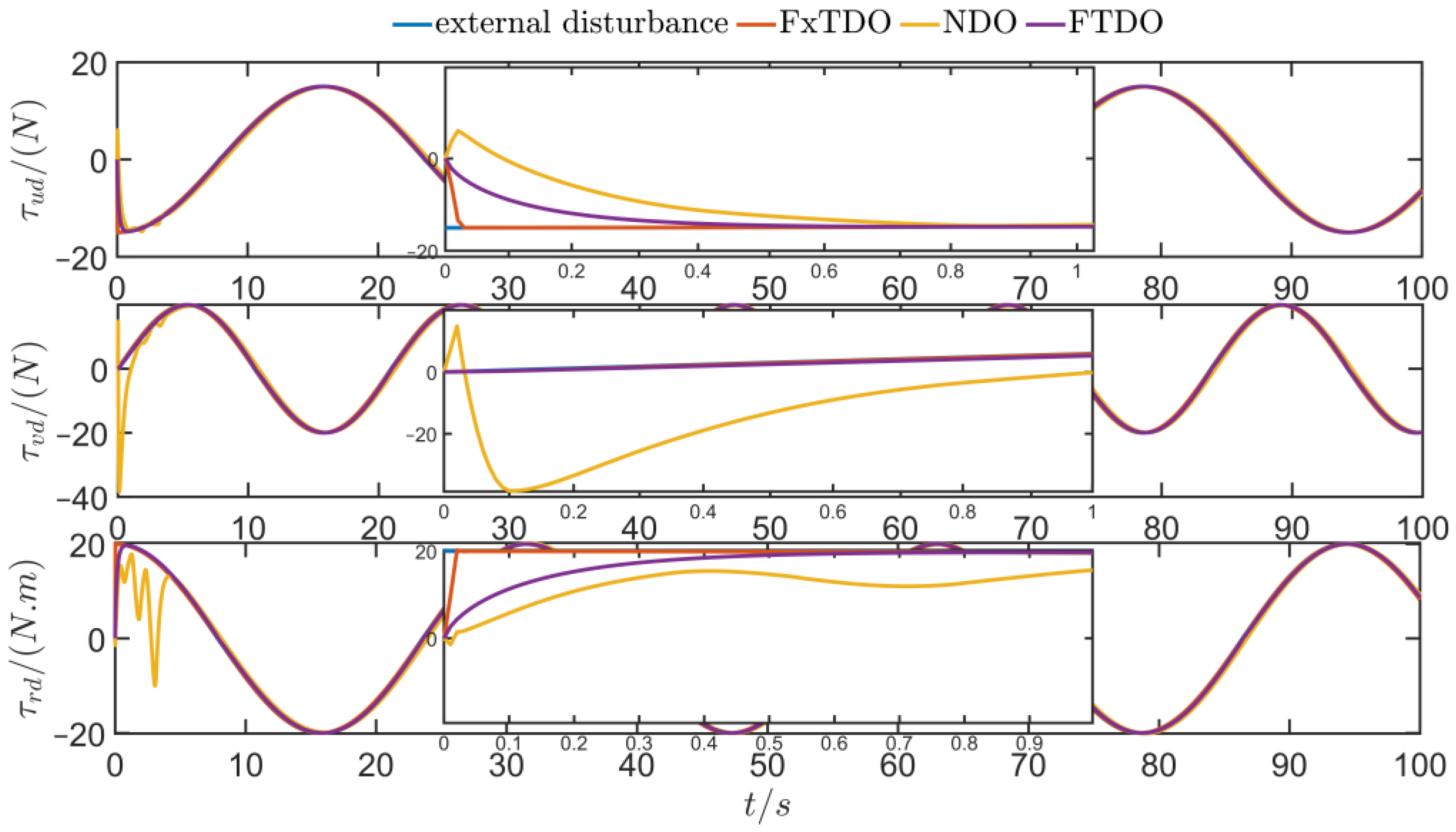
A fixed-time disturbance observer is designed to quickly estimate and compensate for the external time-varying disturbance to improve the controller’s robustness. Different from the existing nonlinear disturbance observer [24] and finite-time disturbance observer [25], the proposed fixed-time observer has faster convergence speed and higher accuracy. Moreover, its convergence time is independent of the initial states.

(2)

In contrast to [21,22], the prescribed performance control technology is introduced to always keep the trajectory tracking error within the preset constraint range to ensure the system’s transient and steady-state performance.

(3)

Combining backstepping control, command filter, and fixed-time control theory, a fixed-time prescribed performance control law is designed to make the trajectory tracking error converge in a fixed time. Unlike the finite-time control [20], the convergence time of the proposed fixed-time control scheme is independent of the system’s initial states.

2. Problem Description and Preliminary Knowledge

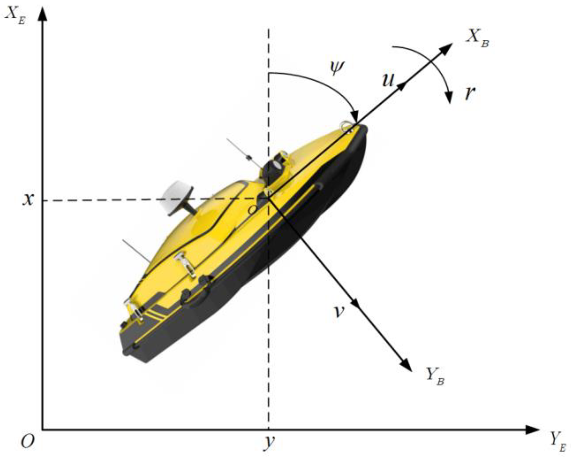
2.1. USV Dynamic Model

This paper studies the trajectory tracking control problem of USVs in two-dimensional horizontal planes. Firstly, to characterize the movement of USVs in two-dimensional space, the geodetic north-east coordinate system $X_{E}O{Y}_E$ and the USV body coordinate system $X_{B}O{Y}_B$ are established. Figure 1 displays the two coordinate systems.

The mathematical model of USV is developed

$$\{\begin{array}{l}\dot{\eta }=J(\psi )\nu ,\\ M\dot{\nu }=-C(\nu )\nu -D(\nu )\nu +{\tau }_p+{\tau }_d\end{array}$$

(1)

where $\eta ={[x,y,\psi ]}^T$ indicates the position and yaw angle of the USV in the geodetic coordinate system; $\nu ={[u,v,r]}^T$ is the forward speed, lateral drift speed, and yaw angular velocity of the USV in the body coordinate system; $J(\psi )$ represents the transfer matrix from the body coordinate to the geodetic coordinate, with the specific form as follows:

$$J(\psi )=\left[\begin{array}{ccc}\cos (\psi )& -\sin (\psi )& 0\\ \sin (\psi )& \cos (\psi )& 0\\ 0& 0& 1\end{array}\right]$$

${\tau }_p\in R^3$ indicates the actual control input vector of USV; ${\tau }_c\in R^3$ represents the command control input vector; ${\tau }_d\in R^3$ is the time-varying external disturbance; and $\Delta \tau ={\tau }_c-{\tau }_p$ represents the difference between the command control input and the actual control input. The relationship between ${\tau }_p$ and ${\tau }_c$ is described as follows

$${\tau }_{pi}=\{\begin{array}{l}sign({\tau }_{ci}){\tau }_{Mi},\left|{\tau }_{ci}\right|\ge {\tau }_{Mi}\\ {\tau }_{ci},\left|{\tau }_{ci}\right|<{\tau }_{Mi}\end{array},i=u,v,r$$

(2)

where ${\tau }_{Mi}$ denotes the maximum force and torque that the thruster can generate in three degrees of freedom; and $sign$ is a sign function. The parameters of inertia matrix $M\in R^3$, Coriolis centripetal force matrix $C\in R^3$, and hydrodynamic damping matrix $D\in R^3$ are shown in [26].

Assumption 1

([27]). The external disturbance ${\tau }_d$ changes slowly and is bounded; that is, there exists a positive constant ${\overline{\tau }}_d$ such that $\Vert {\tau }_d\Vert \le {\overline{\tau }}_d$.

Remark 1.

Given the limited energy exchange in the external marine environment, we can consider the disturbance operating on the USV as an unknown signal that varies over time and is bounded, with a finite rate of change. Therefore, Assumption 1 is valid.

Assumption 2

([28]). The saturation difference $\Delta \tau$ is bounded and satisfies $\Vert \Delta \tau \Vert \le \overline{\tau }$, where $\overline{\tau }$ is a known constant.

2.2. Related Lemmas

Lemma 1

([29]). If there exists a function $V(x):R^m\to R$, $V(x)\ge 0$, $\forall x\in R^m$ and $V(x)=0\iff x=0$, satisfies

$$\dot{V}(x)\le -a{V}^p(x)-b{V}^q(x)$$

(3)

where $a,b>0$, $p\in (0,1)$, $q\in (1,+\infty )$, then the origin of the system is fixed-time stable, and the convergence time $T$ satisfies

$$T\le T_{\max }=\frac{1}{a(1-p)}+\frac{1}{b(q-1)}$$

(4)

Lemma 2

([30]). If there exists a function $V(x):R^m\to R$, $V(x)\ge 0$, $\forall x\in R^m$ and $V(x)=0\iff x=0$, satisfies

$$\dot{V}(x)\le -a{V}^p(x)-b{V}^q(x)+\delta$$

(5)

where $a,b,\delta >0$, $p\in (0,1)$, $q\in (1,+\infty )$, then the origin of the system is practically fixed-time stable, and the convergence time $T$ satisfies

$$T\le T_{\max }=\frac{1}{a\delta (1-p)}+\frac{1}{b\delta (q-1)}$$

(6)

where $\kappa$ is a positive constant, and satisfies $0<\kappa <1$.

Control objectives:

Under Assumptions 1–3, combined with fixed-time disturbance observers (8)–(11), virtual controllers (27), command filters (31), prescribed performance constraints (22), auxiliary dynamics (35), and the fixed-time control law (34), the USV can accurately follow the reference trajectory in a fixed time. The tracking error is always within the prescribed performance constraint range. The mathematical description is as follows:

$$\underset{t\to T}{\lim }\Vert \eta -{\eta }_d\Vert =0, \forall t\ge T$$

(7)

where $\eta \in R^3$ denotes the actual trajectory of USV; ${\eta }_d\in R^3$ represents the reference trajectory; and $T$ is the fixed convergence time.

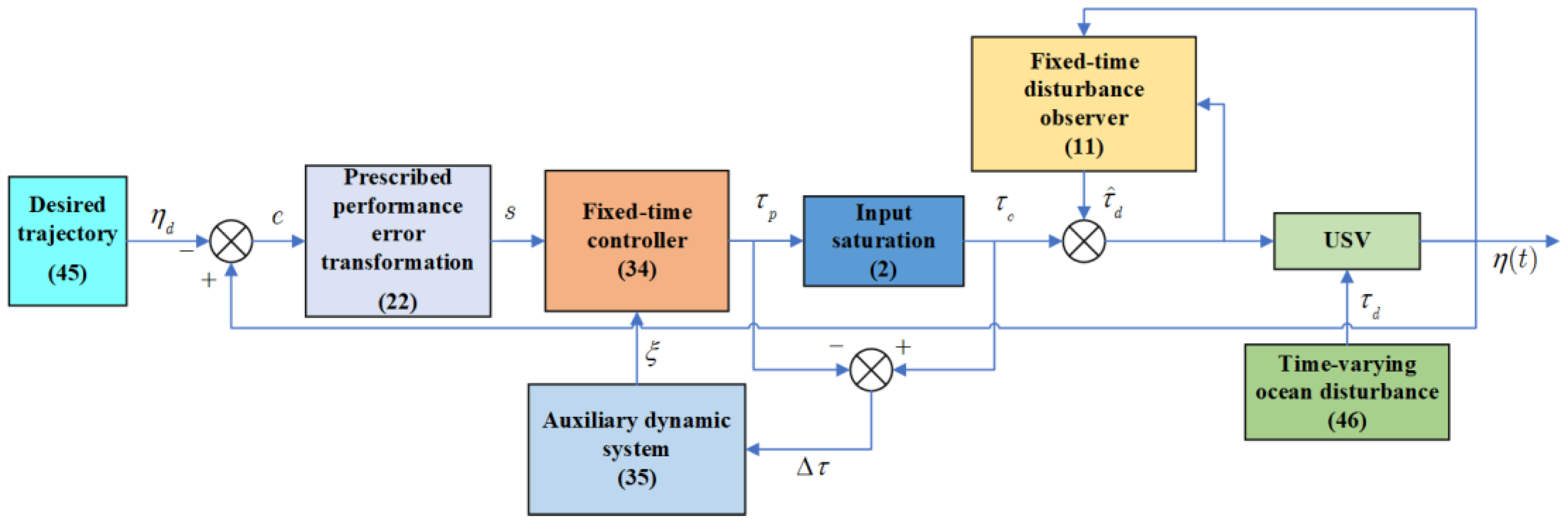
3. Main Results

Initially, a fixed-time disturbance observer is constructed with the purpose of precisely estimating and compensating for the ocean disturbance. Then, the prescribed performance function transforms the unconstrained trajectory tracking error into a constrained state. At the same time, combined with backstepping control, command filter technology, and fixed-time control theory, a fixed-time prescribed performance control law is designed to make the USV accurately follow the reference trajectory in a fixed time.

3.1. Fixed-Time Disturbance Observer Design

First, we define the following auxiliary variables

$$\mathsf{\Phi }=M\nu -\mathsf{ƛ}$$

(8)

The derivative of auxiliary variable $\mathsf{ƛ}$ is structured in the following manner

$$\dot{\mathsf{ƛ}}={\tau }_p-C(\nu )\nu -D(\nu )\nu +{\lambda }_1\mathsf{\Phi }+{\lambda }_2{\mathsf{\Phi }}^{{\gamma }_1}+{\lambda }_3{\mathsf{\Phi }}^{{\gamma }_2}+{\lambda }_{4}sign(\mathsf{\Phi })$$

(9)

where ${\lambda }_i\in R^3,i=1,2,3,4$ is positive definite diagonal matrix. ${\gamma }_1$ and ${\gamma }_2$ are positive constants and satisfy $0<{\gamma }_1<1$, ${\gamma }_2>1$.

Combining Equations (1) and (9), the derivation of Equation (8) can be obtained

$$\begin{array}{l}\dot{\mathsf{\Phi }}=M\dot{\nu }-\dot{\mathsf{ƛ}}=-C(\nu )\nu -D(\nu )\nu +{\tau }_p+{\tau }_d-{\tau }_p+C(\nu )\nu \\ +D(\nu )\nu -{\lambda }_1\mathsf{\Phi }-{\lambda }_2{\mathsf{\Phi }}^{{\gamma }_1}-{\lambda }_3{\mathsf{\Phi }}^{{\gamma }_2}-{\lambda }_{4}sign(\mathsf{\Phi })\\ ={\tau }_d-{\lambda }_1\mathsf{\Phi }-{\lambda }_2{\mathsf{\Phi }}^{{\gamma }_1}-{\lambda }_3{\mathsf{\Phi }}^{{\gamma }_2}-{\lambda }_{4}sign(\mathsf{\Phi })\end{array}$$

(10)

Next, the fixed-time disturbance observer is formulated as

$${\widehat{\tau }}_d={\lambda }_1\mathsf{\Phi }+{\lambda }_2{\mathsf{\Phi }}^{{\gamma }_1}+{\lambda }_3{\mathsf{\Phi }}^{{\gamma }_2}+{\lambda }_{4}sign(\mathsf{\Phi })$$

(11)

Theorem 1.

The designed fixed-time disturbance observers (8)–(11) can accurately estimate the external time-varying disturbance ${\tau }_d$ within a fixed time $T_0$.

Proof. 

The estimation error of observer is defined as

$$\begin{array}{l}{\tilde{\tau }}_d={\tau }_d-{\widehat{\tau }}_d\\ ={\tau }_d-{\lambda }_1\mathsf{\Phi }-{\lambda }_2{\mathsf{\Phi }}^{{\gamma }_1}-{\lambda }_3{\mathsf{\Phi }}^{{\gamma }_2}-{\lambda }_{4}sign(\mathsf{\Phi })\\ =\dot{\mathsf{\Phi }}\end{array}$$

(12)

According to the Equation (12), if $\dot{\mathsf{\Phi }}$ converges, then the observation error ${\tilde{\tau }}_d$ also converges. Therefore, it is only necessary to prove that $\dot{\mathsf{\Phi }}$ convergence can guarantee the convergence of ${\tilde{\tau }}_d$.

We choose the following Lyapunov candidate function

$$V_1=\frac{1}{2}{\mathsf{\Phi }}^T\mathsf{\Phi }$$

(13)

Derivation of the above equation and combining it with Equation (10) can be obtained

$$\begin{array}{l}{\dot{V}}_1={\mathsf{\Phi }}^T\dot{\mathsf{\Phi }}={\mathsf{\Phi }}^T[{\tau }_d-{\lambda }_1\mathsf{\Phi }-{\lambda }_2{\mathsf{\Phi }}^{{\gamma }_1}-{\lambda }_3{\mathsf{\Phi }}^{{\gamma }_2}-{\lambda }_{4}sign(\mathsf{\Phi })]\\ \le -{\lambda }_1({\mathsf{\Phi }}^T\mathsf{\Phi })-{\lambda }_2({\mathsf{\Phi }}^T\mathsf{\Phi }{)}^{\frac{{\gamma }_1+1}{2}}-{\lambda }_3({\mathsf{\Phi }}^T\mathsf{\Phi }{)}^{\frac{{\gamma }_2+1}{2}}\\ \le -{\lambda }_{\min }({\lambda }_2)({\mathsf{\Phi }}^T\mathsf{\Phi }{)}^{\frac{{\gamma }_1+1}{2}}-{\lambda }_{\min }({\lambda }_3)({\mathsf{\Phi }}^T\mathsf{\Phi }{)}^{\frac{{\gamma }_2+1}{2}}\\ =-2^{\frac{{\gamma }_1+1}{2}}{\lambda }_{\min }({\lambda }_2)(\frac{1}{2}{\mathsf{\Phi }}^T\mathsf{\Phi }{)}^{\frac{{\gamma }_1+1}{2}}-2^{\frac{{\gamma }_2+1}{2}}{\lambda }_{\min }({\lambda }_3)(\frac{1}{2}{\mathsf{\Phi }}^T\mathsf{\Phi }{)}^{\frac{{\gamma }_2+1}{2}}\\ =-2^{\frac{{\gamma }_1+1}{2}}{\lambda }_{\min }({\lambda }_2){(V_1)}^{\frac{{\gamma }_1+1}{2}}-2^{\frac{{\gamma }_2+1}{2}}{\lambda }_{\min }({\lambda }_3){(V_1)}^{\frac{{\gamma }_2+1}{2}}\end{array}$$

(14)

As stated in Lemma 1, the auxiliary variable $\mathsf{\Phi }$ is fixed-time stable, so the disturbance estimation error ${\tilde{\tau }}_d$ is also fixed-time stable, and the convergence time $T_0$ satisfies

$$T_0\le T_{\max }:=\frac{2^{\frac{1-{\gamma }_1}{2}}}{{\lambda }_{\min }({\lambda }_2)(1-{\gamma }_1)}+\frac{2^{\frac{{\gamma }_2-1}{2}}}{{\lambda }_{\min }({\lambda }_3)({\gamma }_2-1)}$$

(15)

From the analysis provided above, the following deductions can be made:

$${\tilde{\tau }}_d=0,t\ge T_0$$

(16)

The proof of Theorem 1 is finished. □

3.2. Fixed-Time Prescribed Performance Controller Design

This section presents a control strategy for following a prescribed performance trajectory within a fixed time. The scheme utilizes backstepping control, command filter, fixed-time control theory, and prescribed performance control technology. Figure 2 displays the control block diagram.

(1) Prescribed performance constraints

Define trajectory tracking error

$$e=\eta -{\eta }_d$$

(17)

where $e={[e_1,e_2,e_3]}^T\in R^3$.

Then, the tracking error is constrained within a given range, and the mathematical description is as follows:

$$-e_{i,D}(t)<e_i(t)<e_{i,U}(t), i=1,2,3$$

(18)

where $e_{i,D}(t)$ and $e_{i,U}(t)$ denote the minimum and maximum limits of the preset constraint, respectively, which are defined as follows:

$$e_{i,D}(t)={\delta }_{i,D}{\rho }_i(t),i=1,2,3$$

(19)

$$e_{i,U}(t)={\delta }_{i,U}{\rho }_i(t),i=1,2,3$$

(20)

where ${\delta }_{i,D}$ and ${\delta }_{i,U}$ are positive constants. ${\rho }_i(t)$ represents the prescribed performance function

$${\rho }_i=({\rho }_{i0}-{\rho }_{i\infty })e^{-{\omega }_{i}t}+{\rho }_{i\infty }$$

(21)

where ${\rho }_{i0}$, ${\rho }_{i\infty }$ and ${\omega }_i$ are parameters to be designed.

Assumption 3.

The initial trajectory tracking error of USV satisfies $-e_{i,D}(0)<e_i(0)<e_{i,U}(0), i=1,2,3$.

(2) Error transformation

To fulfill the specified performance requirements of the trajectory tracking system, it is necessary to transform the tracking error in the following manner.

$$s_{1i}=\frac{1}{2}\log (1+\frac{e_i}{e_{i,D}})-\frac{1}{2}\log (1-\frac{e_i}{e_{i,U}}),i=1,2,3$$

(22)

The derivation of the above equation can be obtained

$${\dot{s}}_{1i}=p_i{\dot{e}}_i-q_i{e}_i$$

(23)

where

$$p_i=\frac{1}{2}\left[\frac{1}{e_{i,D}+e_i}+\frac{1}{e_{i,U}-e_i}\right],i=1,2,3$$

(24)

$$q_i=\frac{1}{2}\left[\frac{{\dot{e}}_{i,D}}{e_{i,D}(e_{i,D}+e_i)}+\frac{{\dot{e}}_{i,U}}{e_{i,U}(e_{i,U}-e_i)}\right],i=1,2,3$$

(25)

(3) Controller design

Define the following variables $s_1={[s_{11},s_{12},s_{13}]}^T$, $P=diag(p_1,p_2,p_3)$ and $Q=diag(q_1,q_2,q_3)$.

Therefore, Equation (23) can be rewritten as the following compact form:

$${\dot{s}}_1=P\dot{e}-Qe$$

(26)

As described below, the kinematics controller is constructed:

$${\alpha }_v=J{(\psi )}^T(-P^{-1}(k_1{s_1}^{{\gamma }_1}+k_2{s_1}^{{\gamma }_2})+{\dot{\eta }}_d+P^{-1}Qe)$$

(27)

where $k_1\in R^3$ and $k_2\in R^3$ are positive definite diagonal matrices.

To verify the convergence of $s_1$, consider the following Lyapunov function

$$V_2=\frac{1}{2}{s}_1^T{s}_1$$

(28)

Calculating the above equation’s derivative results in

$$\begin{array}{l}{\dot{V}}_2=s_1^T{\dot{s}}_1\\ =s_1^T(P\dot{e}-Qe)\\ =s_1^T(P(J(\psi )\nu -{\dot{\eta }}_d)-Qe)\end{array}$$

(29)

Substituting Equation (27) into Equation (29) yields

$$\begin{array}{l}{\dot{V}}_2=-s_1^T(k_1{s_1}^{{\gamma }_1}+k_2{s_1}^{{\gamma }_2})\\ =-k_1{(s_1^T{s}_1)}^{\frac{({\gamma }_1+1)}{2}}-k_2{(s_1^T{s}_1)}^{\frac{{\gamma }_2+1}{2}}\\ \le -{\lambda }_{\min }(k_1)2^{\frac{{\gamma }_1+1}{2}}{V}_2^{\frac{{\gamma }_1+1}{2}}-{\lambda }_{\min }(k_2)2^{\frac{{\gamma }_2+1}{2}}{V}_2^{\frac{{\gamma }_2+1}{2}}\end{array}$$

(30)

As Lemma 1 demonstrates, $s_1$ is stable within a fixed time.

To avoid the “differential explosion” problem in backstepping control, the command filter [31] is introduced to obtain new variables ${\alpha }_f$ and ${\dot{\alpha }}_f$, and the mathematical expressions are as follows:

$$\{\begin{array}{l}{\dot{\alpha }}_f=f{\alpha }_g\\ {\dot{\alpha }}_g=-2\iota f{\alpha }_g-f({\alpha }_f-{\alpha }_v)\end{array}$$

(31)

where ${\alpha }_f$ and ${\alpha }_g$ represent the output of the filter; ${\alpha }_v$ is the input. $f>0$ and $\iota \in (0,1]$ are parameters to be designed, which represent the frequency and damping ratio of the filter, respectively, and the initial state of the filter satisfies ${\alpha }_f(0)={\alpha }_v(0)$, $\iota (0)=0$.

Remark 2.

As opposed to the conventional backstepping control approach, the command filtering technique eliminates the need to derive the virtual control law and significantly reduces the algorithm’s computational complexity. This simplifies the controller design and facilitates its implementation in engineering applications.

Next, the speed tracking error is defined.

$$s_2=\nu -{\alpha }_f$$

(32)

By combining Equation (1) and differentiating the aforementioned equation, we obtain

$${\dot{s}}_2=M^{-1}(-C(\nu )\nu -D(\nu )\nu +{\tau }_p+{\tau }_d)-{\dot{\alpha }}_f$$

(33)

We design the following dynamic controller:

$$\begin{array}{l}{\tau }_p=-M(k_3{s_2}^{{\gamma }_1}+k_4{s_2}^{{\gamma }_2}+k_5{s}_2)+C(\nu )\nu \\ +D(\nu )\nu -{\widehat{\tau }}_d+M{\dot{\alpha }}_f+M\xi \end{array}$$

(34)

where $k_3$, $k_4$, and $k_5$ are positive definite matrices and satisfy ${\lambda }_{\min }(k_5)>1$. $\xi$ is an anti-saturation auxiliary dynamic variable, which is structured in the following manner:

$$\dot{\xi }=\{\begin{array}{l}-k_{\xi }{\xi }^{{\gamma }_1}-\frac{\Vert s_2\Delta \tau \Vert +\frac{1}{2}\Delta {\tau }^T\Delta \tau }{{\Vert \xi \Vert }^2}{\xi }^{{\gamma }_2}-k_{\delta }\xi +\Delta \tau ,\Vert \xi \Vert \ge \epsilon \\ \\ \\ 0_{3\times 1},\Vert \xi \Vert <\epsilon \end{array}$$

(35)

where $k_{\xi }\in R^3$ and $k_{\delta }\in R^3$ are positive definite matrices and satisfy ${\lambda }_{\min }(k_{\delta })>1$. $\epsilon >0$ is a constant.

To verify the convergence of $s_2$, consider the following Lyapunov candidate function:

$$V_3=\frac{1}{2}{s}_2^T{s}_2+\frac{1}{2}{\xi }^T\xi$$

(36)

where $V_4=\frac{1}{2}{\xi }^T\xi$.

The differentiation of the above equation results in

$${\dot{V}}_3=s_2^T{\dot{s}}_2+{\dot{V}}_4=s_2^T{\dot{s}}_2+{\xi }^T\dot{\xi }$$

(37)

According to Equations (33) and (34), it can be concluded that

$$\begin{array}{l}{s}_2^T{\dot{s}}_2=s_2^T(-k_3{s_2}^{{\gamma }_1}-k_4{s_2}^{{\gamma }_2}-k_5{s}_2+{\tilde{\tau }}_d+\xi )\\ =-k_3{(s_2^T{s}_2)}^{\frac{{\gamma }_1+1}{2}}-k_4{(s_2^T{s}_2)}^{\frac{{\gamma }_2+1}{2}}-k_5{s}_2^T{s}_2+s_2^T{\tilde{\tau }}_d+s_2^T\xi \\ \le -k_3{(s_2^T{s}_2)}^{\frac{{\gamma }_1+1}{2}}-k_4{(s_2^T{s}_2)}^{\frac{{\gamma }_2+1}{2}}-k_5{s}_2^T{s}_2+\frac{1}{2}{s}_2^T{s}_2\\ +\frac{1}{2}\Vert {\tilde{\tau }}_d\Vert +\frac{1}{2}{s}_2^T{s}_2+\frac{1}{2}{\xi }^T\xi \\ \le -{\lambda }_{\min }(k_3)2^{\frac{{\gamma }_1+1}{2}}{V_2}^{\frac{{\gamma }_1+1}{2}}-{\lambda }_{\min }(k_4)2^{\frac{{\gamma }_2+1}{2}}{V}_2^{\frac{{\gamma }_2+1}{2}}\\ -(k_5-1)s_2^T{s}_2+\frac{1}{2}\Vert {\tilde{\tau }}_d\Vert +\frac{1}{2}{\xi }^T\xi \end{array}$$

(38)

Associative Equation (35) and Young’s inequality are obtained.

$$\begin{array}{l}{\xi }^T\dot{\xi }=-k_{\xi }{({\xi }^T\xi )}^{\frac{{\gamma }_1+1}{2}}\\ -\frac{\left|s_2\Delta \tau \right|+\frac{1}{2}\Delta {\tau }^T\Delta \tau }{{\Vert \xi \Vert }^2}{({\xi }^T\xi )}^{\frac{{\gamma }_2+1}{2}}-k_{\delta }{\xi }^T\xi +{\xi }^T\Delta \tau \\ =-k_{\xi }{({\xi }^T\xi )}^{\frac{{\gamma }_1+1}{2}}-k_{\varpi }{({\xi }^T\xi )}^{\frac{{\gamma }_2+1}{2}}-k_{\delta }{\xi }^T\xi +{\xi }^T\Delta \tau \\ \le -k_{\xi }{({\xi }^T\xi )}^{\frac{{\gamma }_1+1}{2}}-k_{\varpi }{({\xi }^T\xi )}^{\frac{{\gamma }_2+1}{2}}-k_{\delta }{\xi }^T\xi \\ +\frac{1}{2}{\xi }^T\xi +\frac{1}{2}\Vert \Delta \tau \Vert \\ \le -{\lambda }_{\min }(k_{\xi })2^{\frac{{\gamma }_1+1}{2}}{V}_4^{\frac{{\gamma }_1+1}{2}}-{\lambda }_{\min }(k_{\varpi })2^{\frac{{\gamma }_2+1}{2}}{V}_4^{\frac{{\gamma }_2+1}{2}}\\ -k_{\delta }{\xi }^T\xi +\frac{1}{2}{\xi }^T\xi +\frac{1}{2}\Vert \Delta \tau \Vert \end{array}$$

(39)

By combining Equation (36) through (39) with Young’s inequality, we obtain

$$\begin{array}{l}{\dot{V}}_3=s_2^T{\dot{s}}_2+{\xi }^T\dot{\xi }\\ \le -{\lambda }_{\min }(k_3)2^{\frac{{\gamma }_1+1}{2}}{V_2}^{\frac{{\gamma }_1+1}{2}}-{\lambda }_{\min }(k_4)2^{\frac{{\gamma }_2+1}{2}}{V}_2^{\frac{{\gamma }_2+1}{2}}-(k_5-1)s_2^T{s}_2+\frac{1}{2}\Vert {\tilde{\tau }}_d\Vert +\frac{1}{2}{\xi }^T\xi \\ -{\lambda }_{\min }(k_{\xi })2^{\frac{{\gamma }_1+1}{2}}{V}_4^{\frac{{\gamma }_1+1}{2}}-{\lambda }_{\min }(k_{\varpi })2^{\frac{{\gamma }_2+1}{2}}{V}_4^{\frac{{\gamma }_2+1}{2}}-k_{\delta }{\xi }^T\xi +\frac{1}{2}{\xi }^T\xi +\frac{1}{2}\Vert \Delta \tau \Vert \\ \le -{\lambda }_{\min }(k_3)2^{\frac{{\gamma }_1+1}{2}}{V}_2^{\frac{{\gamma }_1+1}{2}}-{\lambda }_{\min }(k_4)2^{\frac{{\gamma }_2+1}{2}}{V}_2^{\frac{{\gamma }_2+1}{2}}\\ -{\lambda }_{\min }(k_{\xi })2^{\frac{{\gamma }_1+1}{2}}{V}_4^{\frac{{\gamma }_1+1}{2}}-{\lambda }_{\min }(k_{\varpi })2^{\frac{{\gamma }_2+1}{2}}{V}_4^{\frac{{\gamma }_2+1}{2}}\\ -(k_5-1)s_2^T{s}_2-(k_{\delta }-1){\xi }^T\xi +\frac{1}{2}\Vert {\tilde{\tau }}_d\Vert +\frac{1}{2}\Vert \Delta \tau \Vert \\ \le -{\lambda }_{\min }(k_3)2^{\frac{{\gamma }_1+1}{2}}{V}_2^{\frac{{\gamma }_1+1}{2}}-{\lambda }_{\min }(k_4)2^{\frac{{\gamma }_2+1}{2}}{V}_2^{\frac{{\gamma }_2+1}{2}}\\ -{\lambda }_{\min }(k_{\xi })2^{\frac{{\gamma }_1+1}{2}}{V}_4^{\frac{{\gamma }_1+1}{2}}-{\lambda }_{\min }(k_{\varpi })2^{\frac{{\gamma }_2+1}{2}}{V}_4^{\frac{{\gamma }_2+1}{2}}+\frac{1}{2}\Vert {\tilde{\tau }}_d\Vert +\frac{1}{2}\Vert \Delta \tau \Vert \end{array}$$

(40)

It can be seen from Lemma 2 that $s_2$ is practically fixed-time stable.

From the above explanation, one can deduce the following theorem.

Theorem 2.

Regarding the issue of trajectory tracking for USVs in the presence of external disturbances and input saturation under Assumptions 1–3, based on the fixed-time disturbance observer (11), the preset performance function constraint (22), the virtual controller (27), the command filter (31), the fixed-time controller (34) and dynamic auxiliary system (35), all the signals of the closed-loop system are fixed-time stable and the convergence time $T<T_0+T_1$, where $T_1$ will be given later. At the same time, by selecting the appropriate parameters, the trajectory tracking error can converge into any small residual set, and the tracking error is always within the prescribed performance constraint.

Proof. 

To demonstrate fixed-time stability of the entire trajectory tracking system, the following Lyapunov candidate function is selected:

$$V=\frac{1}{2}{s}_1^T{s}_1+\frac{1}{2}{s}_2^T{s}_2+\frac{1}{2}{\xi }^T\xi$$

(41)

The above equation can be differentiated to obtain

$$\dot{V}=s_1^T{\dot{s}}_1+s_2^T{\dot{s}}_2+{\xi }^T\dot{\xi }$$

(42)

Based on Equations (30) and (40), it can be inferred that

$$\begin{array}{l}\dot{V}=s_1^T{\dot{s}}_1+s_2^T{\dot{s}}_2+{\xi }^T\dot{\xi }\\ \le -{\lambda }_{\min }(k_1)2^{\frac{{\gamma }_1+1}{2}}{V}_1^{\frac{{\gamma }_1+1}{2}}-{\lambda }_{\min }(k_2)2^{\frac{{\gamma }_2+1}{2}}{V}_1^{\frac{{\gamma }_2+1}{2}}\\ -{\lambda }_{\min }(k_3)2^{\frac{{\gamma }_1+1}{2}}{V_2}^{\frac{{\gamma }_1+1}{2}}-{\lambda }_{\min }(k_4)2^{\frac{{\gamma }_2+1}{2}}{V_2}^{\frac{{\gamma }_2+1}{2}}\\ -{\lambda }_{\min }(k_{\xi })2^{\frac{{\gamma }_1+1}{2}}{V}_4^{\frac{{\gamma }_1+1}{2}}-{\lambda }_{\min }(k_{\varpi })2^{\frac{{\gamma }_2+1}{2}}{V}_4^{\frac{{\gamma }_2+1}{2}}\\ +\frac{1}{2}\Vert {\tilde{\tau }}_d\Vert +\frac{1}{2}\Vert \Delta \tau \Vert \end{array}$$

(43)

where $a=2^{\frac{{\gamma }_1+1}{2}}{\lambda }_{\min }\left\{k_1,k_3,k_{\xi }\right\}$; $b=2{\lambda }_{\min }\left\{k_2,k_4,k_{\varpi }\right\}$; $\delta =\frac{1}{2}\Vert {\tilde{\tau }}_d\Vert +\frac{1}{2}\Vert \Delta \tau \Vert$. The convergence time $T_1$ satisfies the following inequality

$$T_1\le T_{\max }:=\frac{2}{a\delta (1-{\gamma }_1)}+\frac{2}{b\delta (1-{\gamma }_2)}$$

(44)

The proof of Theorem 2 is complete. □

Remark 3.

The fixed-time trajectory tracking control strategy presented in this research guarantees that the tracking error converges within a fixed time and the convergence time is independent of the initial state and only related to the control parameters. Although the control scheme can theoretically achieve tracking control at any time by adjusting the control parameters, the convergence time cannot be changed arbitrarily due to the actual existence of USV (such as thruster saturation, input limitation, etc.). According to the maximum output of the propulsion system, the convergence time has a minimum lower bound.

4. Simulation Results

Within this section, MATLAB R2022a is utilized to conduct relevant experiments using a PC equipped with an AMD Ryzen 7 5800H CPU and 16 GB memory. Furthermore, the simulation experiments utilize the CybershipⅡvessel model, which was developed by the Norwegian University of Science and Technology. The precise model parameters refer to reference [26].

4.1. Simulation Conditions

To thoroughly validate the tracking performance of the proposed control scheme, the reference trajectory is created in the following manner.

$${\eta }_d=\left[\begin{array}{l}{x}_d\\ y_d\\ {\psi }_d\end{array}\right]=\left[\begin{array}{l}20\sin (0.025\pi t)\\ 9\sin (0.05\pi t)\\ 0.05t\end{array}\right]$$

(45)

The external time-varying disturbance is designed as

$${\tau }_d=\left[\begin{array}{l}{\tau }_{ud}\\ {\tau }_{vd}\\ {\tau }_{rd}\end{array}\right]=\left[\begin{array}{l}-15\cos (0.2t)\\ 20\sin (0.3t)\\ 20\cos (0.2t)\end{array}\right]$$

(46)

The initial pose vector and velocity vector of the USV are set to ${\eta }_0={[2,-5,\frac{\pi }{18}]}^T$, $\nu ={[0,0,0]}^T$. Set the prescribed performance parameters to ${\delta }_{i,D}={\delta }_{i,U}=1$, $e_{1,U}=e_{2,U}=-e_{1,D}=-e_{2,D}=(8-0.3)e^{-0.1t}+0.3$, $e_{3,U}=-e_{3,D}=(\frac{\pi }{9}-\frac{\pi }{240})e^{-0.1t}+\frac{\pi }{240}$.

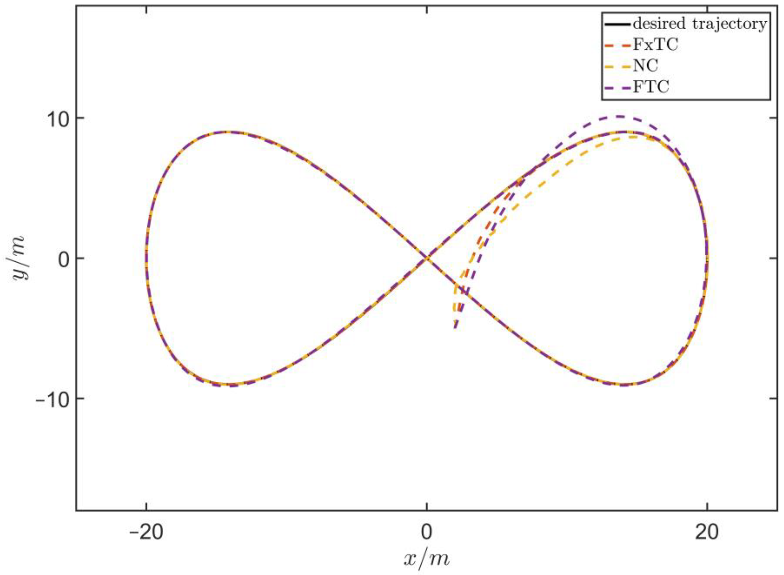
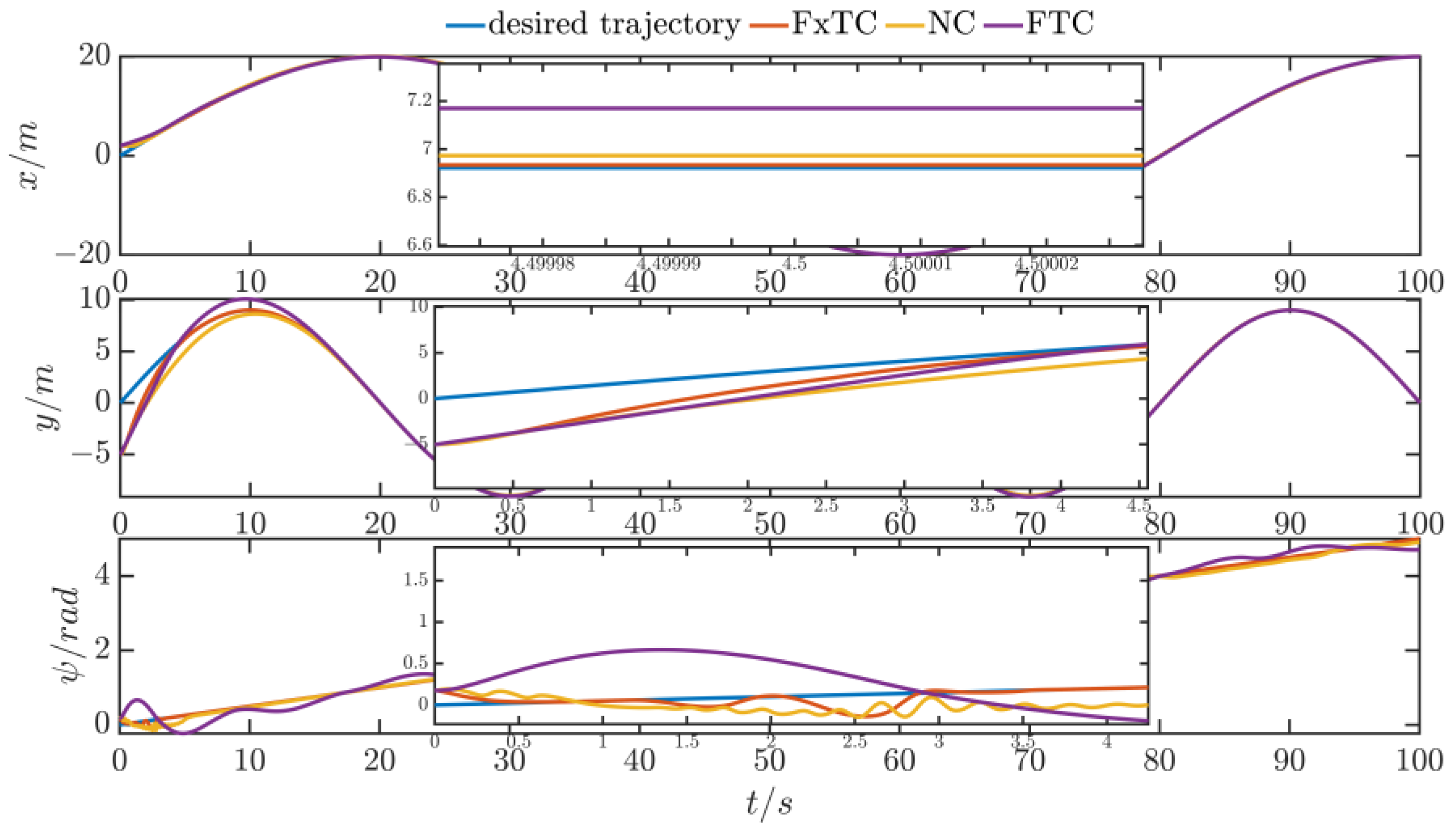
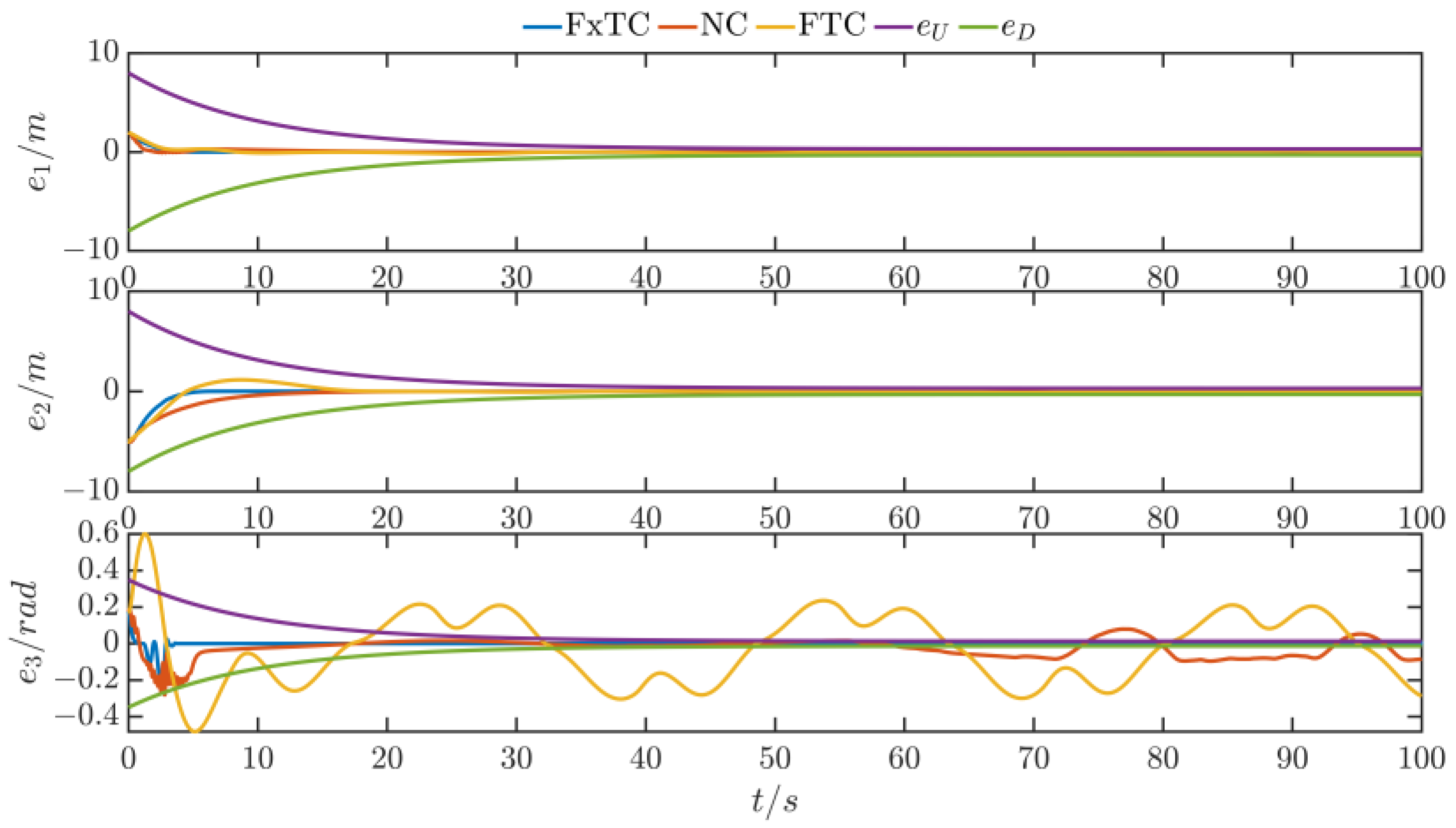
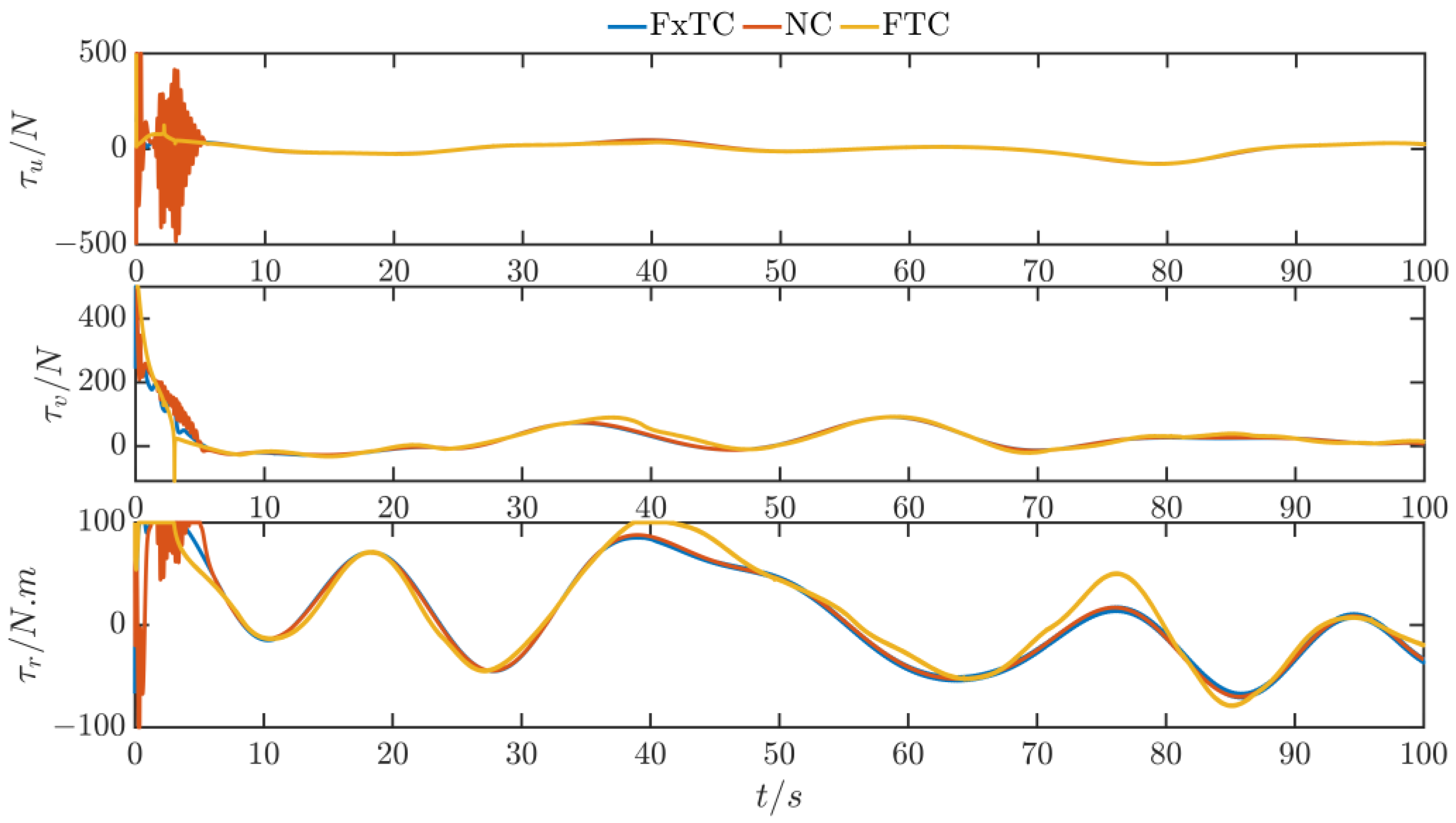
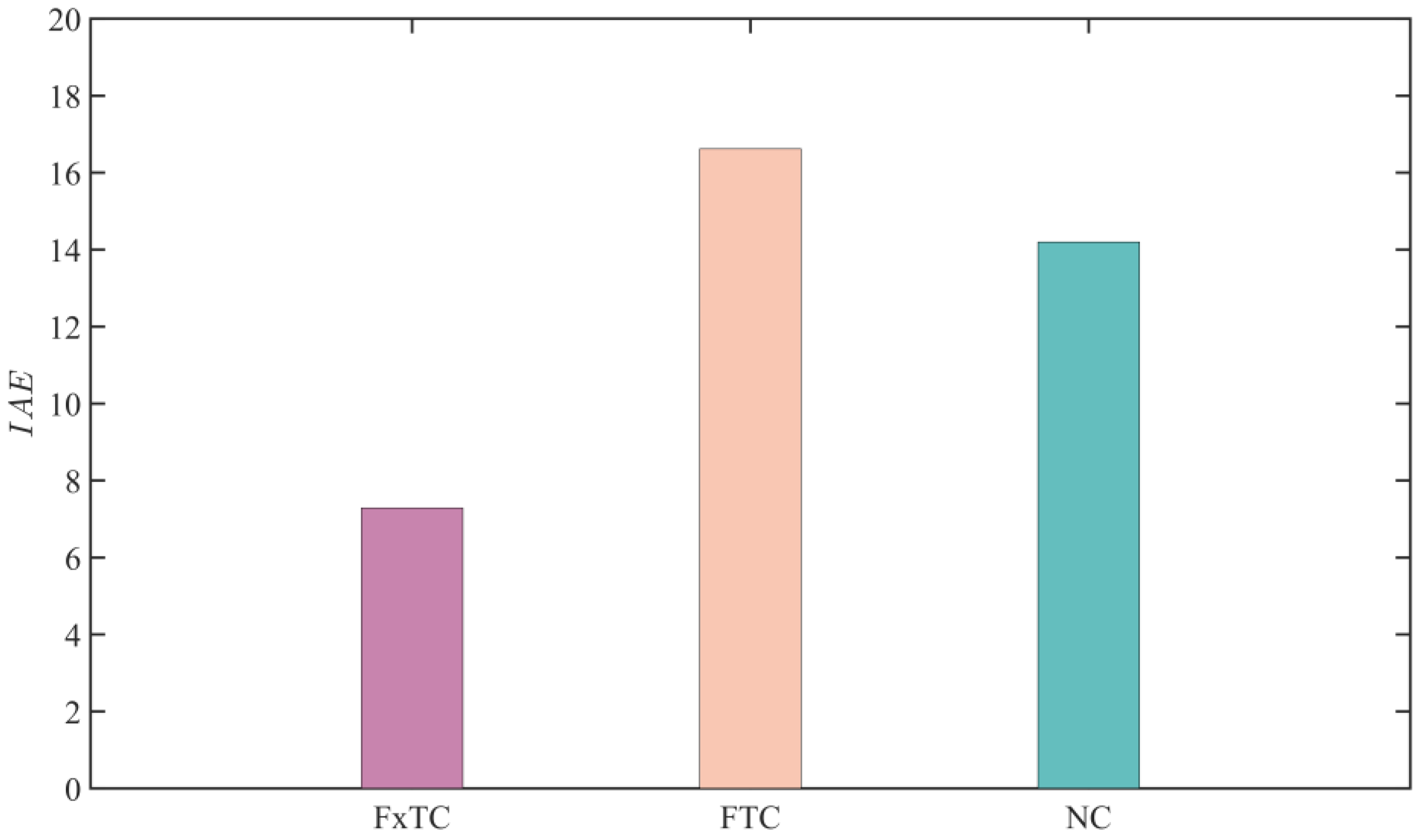
4.2. Simulation Results

To validate the superiority of the fixed-time disturbance observer discussed in this study, it is contrasted with observers mentioned in [24,25]. The specific forms of the nonlinear disturbance observer in [24] and the finite-time disturbance observer in [25] are shown in Equations (47) and (48), respectively.

$$\{\begin{array}{l}{\widehat{\tau }}_d=\theta +KM\nu \\ \dot{\theta }=-K\theta -K(-D(\nu )\nu +{\tau }_p+KM\nu )\end{array}$$

(47)

where $\theta$ is the auxiliary variable of the observer; $K\in R^{3\times 3}$ denotes a positive definite diagonal matrix parameter, and the specific parameter design is the same as that in ref. [24].

$$\{\begin{array}{l}{\widehat{\tau }}_d=K_{1}si{g}^{{\sigma }_1}(\rho )+K_2{\displaystyle \int si{g}^{{\sigma }_2}(\rho )}dt\\ \rho =M\nu -M\widehat{\nu }\end{array}$$

(48)

where both $K_1\in R^{3\times 3}$ and $K_2\in R^{3\times 3}$ are positive definite parameter matrices; ${\sigma }_1$ and ${\sigma }_2$ satisfy $0.5<{\sigma }_1<1$, ${\sigma }_2=2{\sigma }_1-1$, $si{g}^{\sigma }(\cdot )={|\cdot |}^{\sigma }sign(\cdot )$; the specific parameter design is the same as that in [25].

The parameter settings of the disturbance observer in this paper are as follows: ${\lambda }_1=diag\left(5,5,5\right)$, ${\lambda }_2=diag\left(\frac{5}{7},\frac{5}{7},\frac{5}{7}\right)$, ${\lambda }_3=diag\left(\frac{3}{5},\frac{3}{5},\frac{3}{5}\right)$, ${\lambda }_4=diag\left(6,5,6\right)$, ${\gamma }_1=\frac{5}{7}$,${\gamma }_2=\frac{5}{3}$. The initial states of the three disturbance observers are set to ${[0,0,0]}^T$. Figure 3 displays the simulation findings. In the initial observation stage, the estimation of the nonlinear disturbance observer (NDO) in [24] has a significant overshoot, and the disturbance observation error is large. Although the finite-time disturbance observer (FTDO) in [25] has no overshoot problem, the convergence time is slower than that of the fixed-time disturbance observer (FxTDO) in this paper, and the convergence time is affected by the initial state. Therefore, compared with [24,25], the fixed-time disturbance observer in this paper can quickly and accurately estimate the disturbance within a fixed time $T_0$, with higher accuracy and timeliness.

In addition, to validate the superiority of the fixed-time tracking control (FxTC) scheme proposed in this research, the nonlinear controller (NC) (49) in [32] and the finite-time controller (FTC) (50) in [19] are compared and analyzed. The specific forms of the above two controllers are as follows.

$$\tau =C(\nu )\nu +D(\nu )\nu +M{\dot{\nu }}_d-sign(s_2){\overline{\tau }}_d-J^T(\psi )s_1-K_2{s}_2$$

(49)

where ${\overline{\tau }}_d$ is the upper bound of unknown time-varying disturbance; $K_2\in R^{3\times 3}$ is the positive definite diagonal parameter matrix to be designed; and the specific parameter design is the same as that in [32].

$$\tau =C(\nu )\nu +D(\nu )\nu +M\dot{\beta }-J^T{s}_1-k_{2}c-{\tau }_d-c{\left|s_2\right|}^{\gamma }sign(s_2)$$

(50)

where $k_2$ is the positive definite parameter matrix to be designed; $c$ and $\gamma$ are positive constants and satisfy $0<\gamma <1$; and the specific parameter design is the same as that in ref. [19].

The proposed controller parameter in this paper is set to $k_1=k_3=diag\left(\frac{5}{7},\frac{5}{7},\frac{5}{7}\right)$, $k_2=k_4=diag\left(\frac{3}{5},\frac{3}{5},\frac{3}{5}\right)$, $k_5=diag\left(5,5,5\right)$. The maximum value of the force and torque generated by the USV propulsion system in all directions is set to ${\tau }_{u,\max }=500N$, ${\tau }_{v,\max }=500N$, ${\tau }_{r,\max }=100N$.

The simulation results are as follows: Figure 4 compares trajectory tracking under the above three controllers. It can be seen from the Figure 4 that compared with [32,19], the proposed fixed-time prescribed performance controller can make the USV track the desired trajectory faster, and the tracking error is the smallest. Figure 5 shows the tracking components of three different controllers on three degrees of freedom. The fixed-time controller (FxTC) in this paper has better tracking performance. Figure 6 shows the trajectory tracking error curves under the three control effects. It can be seen from Figure 6 that the yaw angle tracking error under the finite-time controller (FTC) in [19] fluctuates wildly and cannot converge to the preset performance constraint range in finite time. Although the yaw angle error under the action of the nonlinear controller (NC) in [32] can achieve convergence, there is a significant overshoot, and the yaw angle error also exceeds the prescribed performance constraints. The trajectory tracking error under the controller’s action in this paper can converge quickly in a fixed time and remain within the preset constraint range to achieve fast and accurate trajectory tracking control. Figure 7 shows the control input variation curves of three controllers. For fairness, the controller in [32] and [19] are treated with the same anti-saturation treatment as in this paper. However, according to Figure 7, the controller in [32] has a severe oscillation in the initial stage of control, which is not conducive to the regular operation of the propeller. In addition, although the fluctuation range of the controller in [19] is small, the control force or torque is large, which will increase the controller’s energy consumption. In this paper, the control fluctuation is relatively stable and always within the preset limit value.

To confirm the efficiency and superiority of the control scheme proposed in this work, integrated absolute errors (IAE) are employed as the performance index to measure the control performance of the three different controllers. The mathematical description of IAE is as follows

$$IAE=\sum {\displaystyle {\int }_0^t\left|e_i\right|}dt,i=1,2,3$$

(51)

where $t$ is the simulation time.

According to Figure 8, the IAE values of the control scheme in this paper, refs. [19,32] are 7.29, 14.20, and 16.62, respectively. Hence, the IAE values of the control scheme presented in this article are comparatively lower than the values reported in [19,32]. This implies that the control scheme described in this paper exhibits superior accuracy. To summarize, the control technique suggested in this research for tracking performance trajectories with fixed-time presets has a faster convergence speed and superior tracking performance.

5. Conclusions

This work presents a fixed-time prescribed performance control strategy to address the issue of precise trajectory tracking control of autonomous surface vehicles in the presence of external interference and input saturation. Firstly, a fixed-time disturbance observer is created to counteract the impact of external disturbances, while an anti-windup auxiliary dynamic is implemented to successfully address the problem of actuator saturation. Furthermore, to guarantee both the transient and steady-state performance of the trajectory tracking system, we have implemented preset performance control technology. This technology ensures that the tracking error always remains within the prescribed performance constraint range, thereby enhancing the accuracy of trajectory tracking. Finally, the Lyapunov stability theory is employed to validate the fixed-time stability of the proposed control scheme. In addition, simulation experiments were designed to compare three different controllers. The findings indicate that the IAE value of the control method introduced in this study is 56.1% and 48.71% less than the IAE values of the finite time controller in [19] and the nonlinear controller in [32], respectively. The results clearly indicate the reliability and superiority of the control strategy proposed in this research.

References

- Jiang, K.; Mao, L.; Su, Y.; Zheng, Y. Trajectory tracking control for underactuated USV with prescribed performance and input quantization. Symmetry 2021, 13, 2208. [Google Scholar] [CrossRef]
- Qin, J.; Du, J. Robust adaptive asymptotic trajectory tracking control for underactuated surface vessels subject to unknown dynamics and input saturation. J. Mar. Sci. Technol. 2022, 27, 307–319. [Google Scholar] [CrossRef]
- Xiaoming, C.A.O.; Yong, W.; Hui, H.; Zhipeng, S.H.E.N. Dynamic surface backstepping trajectory tracking control of unmanned underwater vehicles with ocean current disturbances. Syst. Eng. Electron. 2021, 43, 1664–1672. (In Chinese) [Google Scholar]
- Shen, Z.; Wang, Q.; Dong, S.; Yu, H. Prescribed performance dynamic surface control for trajectory-tracking of unmanned surface vessel with input saturation. Appl. Ocean Res. 2021, 113, 102736. [Google Scholar] [CrossRef]
- Wang, H.; Dong, Z.; Qi, S.; Zhang, Z.; Zhang, H. Trajectory-tracking control of an underactuated unmanned surface vehicle based on quasi-infinite horizon model predictive control algorithm. Trans. Inst. Meas. Control 2022, 44, 2709–2718. [Google Scholar] [CrossRef]
- Abdelaal, M.; Fränzle, M.; Hahn, A. Nonlinear Model Predictive Control for trajectory tracking and collision avoidance of underactuated vessels with disturbances. Ocean Eng. 2018, 160, 168–180. [Google Scholar] [CrossRef]
- Lv, C.; Yu, H.; Chen, J.; Zhao, N.; Chi, J. Trajectory tracking control for unmanned surface vessel with input saturation and disturbances via robust state error IDA-PBC approach. J. Frankl. Inst. 2022, 359, 1899–1924. [Google Scholar] [CrossRef]
- Wu, G.X.; Ding, Y.; Tahsin, T.; Atilla, I. Adaptive neural network and extended state observer-based non-singular terminal sliding mode tracking control for an underactuated USV with unknown uncertainties. Appl. Ocean. Res. 2023, 135, 103560. [Google Scholar] [CrossRef]
- Dong, Z.; Wan, L.; Li, Y.; Liu, T.; Zhang, G. Trajectory tracking control of underactuated USV based on modified backstepping approach. Int. J. Nav. Archit. Ocean Eng. 2015, 7, 817–832. [Google Scholar] [CrossRef]
- Zhang, K.Q.; Zhou, X.F.; Meng, X.H.; Zhou, H.B. Three-dimensional integrated guidance and control design with fixed-time convergence. J. Beijing Univ. Aeronaut. Astronaut. 2023, 49, 842–852. (In Chinese) [Google Scholar]
- Swaroop, D.; Hedrick, J.K.; Yip, P.P.; Gerdes, J.C. Dynamic surface control for a class of nonlinear systems. IEEE Trans. Autom. Control 2000, 45, 1893–1899. [Google Scholar] [CrossRef]
- Shen, Z.P.; Zhang, X.L.; Zhang, N. Recursive sliding mode dynamic surface output feedback control for ship trajectory tracking based on neural network observer. Control Theory Appl. 2018, 35, 1092–1100. (In Chinese) [Google Scholar]
- Cao, X.F.; Liu, S.F.; Shi, G.Y.; Li, C.H. Trajectory tracking of unmanned surface vehicle based on model predictive control. Ship Eng. 2023, 45, 354–357. (In Chinese) [Google Scholar]
- Chen, Z.; Zhang, Y.; Nie, Y.; Tang, J.; Zhu, S. Adaptive sliding mode control design for nonlinear unmanned surface vessel using RBFNN and disturbance-observer. IEEE Access 2020, 8, 45457–45467. [Google Scholar] [CrossRef]
- Wang, N.; Gao, Y.; Shuailin, L.; Joo, M.E. Integral sliding mode based finite-time trajectory tracking control of unmanned surface vehicles with input saturations. Indian, J. Geo-Mar. Sci. 2017, 46, 2493–2501. [Google Scholar]
- Zhao, J.; Cai, C.T.; Qiao, R.J. Finite-time dynamic prescribed performance control for surface unmanned vehicles with unknow disturbance. CAAI Trans. Intell. Syst. 2023, 18, 849–857. (In Chinese) [Google Scholar]
- Polyakov, A. Nonlinear feedback design for fixed-time stabilization of linear control systems. IEEE Trans. Autom. Control 2011, 57, 2106–2110. [Google Scholar] [CrossRef]
- Wang, N.; Wang, R.H.; Lu, T. Fixed-time precision tracking control of an unmanned surface vehicle constrained by thruster saturations. Control Theory Appl. 2023, 40, 55–64. (In Chinese) [Google Scholar]
- Dai, Y.; Yang, C.; Yu, S.; Mao, Y.; Zhao, Y. Finite-time trajectory tracking for marine vessel by nonsingular backstepping controller with unknown external disturbance. IEEE Access 2019, 7, 165897–165907. [Google Scholar] [CrossRef]
- Xu, D.; Liu, Z.; Song, J.; Zhou, X. Finite time trajectory tracking with full-state feedback of underactuated unmanned surface vessel based on nonsingular fast terminal sliding mode. J. Mar. Sci. Eng. 2022, 10, 1845. [Google Scholar] [CrossRef]
- Liu, W.; Ye, H.; Yang, X. Super-twisting sliding mode control for the trajectory tracking of underactuated USVs with disturbances. J. Mar. Sci. Eng. 2023, 11, 636. [Google Scholar] [CrossRef]
- Gao, Z.; Guo, G. Command-filtered fixed-time trajectory tracking control of surface vehicles based on a disturbance observer. Int. J. Robust Nonlinear Control 2019, 29, 4348–4365. [Google Scholar] [CrossRef]
- Jiang, T.; Yan, Y.; Yu, S.H. Adaptive sliding mode control for unmanned surface vehicles with predefined-time tracking performances. J. Mar. Sci. Eng. 2023, 11, 1244. [Google Scholar] [CrossRef]
- Feng, N.; Wu, D.; Yu, H.; Yamashita, A.S.; Huang, Y. Predictive compensator-based event-triggered model predictive control with nonlinear disturbance observer for unmanned surface vehicle under cyber-attacks. Ocean Eng. 2022, 259, 111868. [Google Scholar] [CrossRef]
- Liu, C.; Han, X.; Sun, C.; Chen, X.; Shao, X. Adaptive dynamic positioning control of an offshore wind turbine installation vessel subjected to thruster dynamics and input constraints. Ocean Eng. 2024, 292, 116516. [Google Scholar] [CrossRef]
- Skjetne, R.; Fossen, T.I.; Kokotović, P.V. Adaptive maneuvering, with experiments, for a model ship in a marine control laboratory. Automatica 2005, 41, 289–298. [Google Scholar] [CrossRef]
- Zhu, G.; Du, J. Global robust adaptive trajectory tracking control for surface ships under input saturation. IEEE J. Ocean. Eng. 2018, 45, 442–450. [Google Scholar] [CrossRef]
- Cao, S.; Sun, L.; Jiang, J.; Zuo, Z. Reinforcement learning-based fixed-time trajectory tracking control for uncertain robotic manipulators with input saturation. IEEE Trans. Neural Netw. Learn. Syst. 2023, 34, 4584–4595. [Google Scholar] [CrossRef]
- Gao, Z.Y.; Guo, G. Fixed-time formation control of AUVs based on a disturbance observer. Acta Autom. Sin. 2019, 45, 1094–1102. (In Chinese) [Google Scholar]
- Sun, M.W.; Ren, L.; Liu, J.; Sun, C.Y. Dynamic event-triggered fixed-time consensus control of multi-agent systems under switching topologies. Acta Autom. Sin. 2023, 49, 1295–1305. (In Chinese) [Google Scholar]
- Farrell, J.A.; Polycarpou, M.; Sharma, M.; Dong, W. Command filtered backstepping. IEEE Trans. Autom. Control 2009, 54, 1391–1395. [Google Scholar] [CrossRef]
- Zhang, X.L.; Shen, Z.P.; Bi, Y.N. Adaptive dynamic surface sliding mode control for ship trajectory tracking with disturbance observer. Ship Eng. 2018, 40, 81–87. (In Chinese) [Google Scholar]
Disclaimer/Publisher’s Note: The statements, opinions and data contained in all publications are solely those of the individual author(s) and contributor(s) and not of MDPI and/or the editor(s). MDPI and/or the editor(s) disclaim responsibility for any injury to people or property resulting from any ideas, methods, instructions or products referred to in the content. |
© 2024 by the authors. Licensee MDPI, Basel, Switzerland. This article is an open access article distributed under the terms and conditions of the Creative Commons Attribution (CC BY) license (https://creativecommons.org/licenses/by/4.0/).
Share and Cite
Sui, B.; Zhang, J.; Liu, Z.; Wei, J. Fixed-Time Trajectory Tracking Control of Fully Actuated Unmanned Surface Vessels with Error Constraints. J. Mar. Sci. Eng. 2024, 12, 584. https://0-doi-org.brum.beds.ac.uk/10.3390/jmse12040584
Sui B, Zhang J, Liu Z, Wei J. Fixed-Time Trajectory Tracking Control of Fully Actuated Unmanned Surface Vessels with Error Constraints. Journal of Marine Science and Engineering. 2024; 12(4):584. https://0-doi-org.brum.beds.ac.uk/10.3390/jmse12040584
Chicago/Turabian StyleSui, Bowen, Jianqiang Zhang, Zhong Liu, and Junbao Wei. 2024. "Fixed-Time Trajectory Tracking Control of Fully Actuated Unmanned Surface Vessels with Error Constraints" Journal of Marine Science and Engineering 12, no. 4: 584. https://0-doi-org.brum.beds.ac.uk/10.3390/jmse12040584