High-Resistance Connection Fault Diagnosis in Ship Electric Propulsion System Using Res-CBDNN

Abstract

The fault detection and diagnosis of a ship’s electric propulsion system is of great significance to the reliability and safety of large modern ships. The traditional fault diagnosis method based on mathematical models and expert knowledge is limited by the difficulty of establishing an accurate model of the complex system, and it is easy to cause false alarms. Data-driven methods, such as deep learning, can automatically learn from the mass of data, extract and analyze fault characteristics, and create a more objective distinction system state. A deep learning fault diagnosis model based on ResNet feature extraction capability and bidirectional long-term memory network timing processing capability is proposed to realize fault diagnosis of high resistance connections in ship electric propulsion systems. The results show that the res-convolutional BiLSTM deep neural network (Res-CBDNN) can fully integrate the advantages of the two networks, efficiently process fault current data, and achieve high-performance fault diagnosis. The accuracy of Res-CBDNN can be kept above 85% in a noisy environment, and it can effectively monitor the high resistance connection fault of ship electric propulsion systems.

1. Introduction

Permanent magnet synchronous motors (PMSMs) have the characteristics of high-power density, fast response, and large torque, making them the main propulsion motors in all-electric marine propulsion systems. However, adverse factors such as a bad working environment, high temperature and humidity, and narrow working space affect the safety and reliability of the marine propulsion system [1]. High-resistance connection (HRC) is a kind of low probability, high-cost fault in marine electric propulsion systems, which is mainly caused by the instability of the power supply due to the corrosion, vibration, or weak connection of the stator end of the propulsion motor. In the worst-case scenario, the fault may evolve into an open-phase fault (OPF), causing a catastrophic loss of power and requiring early identification and control of its spread [2]. It is difficult to realize the effective identification and rapid location of HRC early faults in ship electric propulsion fault diagnosis.

To realize HRC fault diagnosis by an electrical parameter, the zero sequence current component (ZSCC) and zero sequence voltage component (ZSVC) are used as HRC fault signals. Hang. J [3] calculated the angle difference between ZSCC and stator current for online HRC fault diagnosis, but the use of a PMSM system with a triangle connection was limited. Based on this, ZSVC and current were used to solve the resistance deviation and realize the HRC fault location in [4], but it was impossible to distinguish between turn-to-turn short circuit and HRC fault. A high-frequency component was used to distinguish between a turn-short circuit and HRC fault in [5], and the ZSVC was analyzed to detect HRC fault by the amplitude of the fundamental frequency component and complete fault location [6]; however, it was not suitable for HRC fault diagnosis of the ship’s electric propulsion system, which is a compact system, because it failed to draw the neutral point of the motor and configure additional resistance networks and instruments to detect the zero sequence current and voltage.

To avoid adding additional sensors, Mengoni [7] extended the vector analysis method to the field of motor control by referring to the three-phase unbalanced theory of power systems. HRC fault diagnosis was realized by calculating unbalanced resistance with the current amplitude and voltage vector. In [8], based on magnetic field swing technology, the vector oscillation angle of the fault current was analyzed, the feature of the fault current was extracted by the symmetrical component method, and the fault degree was judged by a three-phase unbalanced degree. These methods have high diagnostic ability, but their calculation methods are complex and cannot detect the initial HRC weak fault, so their application range is limited. Most scholars use the model reference method, which is easy to realize in the control system, to diagnose the HRC fault by establishing the system mechanism model, calculating the theoretical output, and taking the deviation from the actual data as the fault diagnosis basis. Goucalves [9] distinguished HRC and OPF faults by referring to the second component of current error, but it was not suitable for marine electric propulsion systems because of its poor diagnosis effect in the low-speed segment. In [10], the voltage distortion caused by HRC was taken as the fault characteristic, and a fault indicator insensitive to motor parameters was designed to diagnose and locate the fault, but the influence of the current controller was not considered. The second order component of the voltage control signal of the d-q axis was taken as the fault index in [11] to solve this problem so that the fault diagnosis could be realized; therefore, a wider control band-width was needed, which required the high performance of the controller. The model reference method can realize HRC fault location and degree estimation to a certain extent. Still, its diagnosis results are influenced by the model accuracy and control system performance, but its practicability is limited due to the influence of model accuracy and control system performance. In addition, the high-frequency signal injection method [12,13,14] is also prevalent nowadays, but this method belongs to intrusion detection. The high-frequency signal injection causes the torque to ripple, affecting the dynamic performance of the system and reducing its reliability.

Because of the high cost and low efficiency, traditional fault diagnosis technology based on mathematical models and expert knowledge cannot meet the accuracy requirements of the self-healing control system of marine electric propulsion systems. Machine learning (ML) is a kind of modeling technology that can effectively avoid the influence of model precision and professional knowledge on diagnosis results. Gonzalez [15] used the random forest method to train the network with fault data, establish the diagnosis model, and realize the fault diagnosis of the induction motor. Allafi [16] used linear discriminant analysis to reduce the dimension of voltage second harmonic data, first by support vector machines (SVM) to detect fault types and then by K-nearest neighbor (KNN) to identify the extent of the fault. This data-driven method is suitable for fault diagnosis of complex nonlinear systems such as the marine electric propulsion system.

Given the strong interference of the marine electric propulsion system and the highly complex electrical system, early fault identification and rapid location are common difficulties in the field of fault diagnosis. In this paper, the deep learning method is used to diagnose HRC of complex progressive failure. A Res-CBDNN deep learning network is designed to diagnose the faults of marine electric propulsion systems based on the characteristics of cyclic networks and deep networks. According to the output current and torque data of the inverter in the propulsion system, the fault characteristic information is mined by the convolutional neural network connected by the residual error, and a bidirectional long-term and short-term neural network is used to extract and identify the fault periodicity. The robustness and accuracy of the proposed method are verified by different noise pollution data. The results show that the proposed method not only improves the accuracy of fault location but also resists noise disturbance and improves the accuracy and robustness of diagnosis.

2. HRC Fault Analysis of Ship Electric Propulsion System

2.1. Structure of Shipboard Main Power System

With the increase in ship power capacity, most modern shipboard power systems use multiple gas turbines or diesel synchronous generator sets to coordinate with the regional distribution network topology. The medium-voltage district distribution system supplies power to the ship’s electric propulsion units via a zone distribution board (ZSB) and a propulsion distribution board (PSB). Figure 1 shows the main power unit structure of an electrically propulsed ship.

The main distribution board is composed of the generator control panel, synchronous panel, load panel, and bus bar. The propulsion area distribution board is used as a power distribution board to supply energy for the medium-voltage propulsion system. The area distribution panel supplies power to the ship’s low-voltage equipment and lighting.

Due to the harsh conditions during navigation, the ship’s electric propulsion system requires high stability and reliability [17]; therefore, accurate diagnostic methods must be developed, and data support must be provided to enable fault tolerance and maintenance strategies. This paper examines the early HRC fault characteristics of the three-phase electric propulsion system of ships using a deep-learning diagnosis method.

2.2. HRC Fault Analysis of Electric Propulsion System

The HRC fault of the ship propulsion system, which usually occurs between the drive inverter circuit and the propulsion motor, is a discontinuous early gradual fault [18], and its failure schematic is shown in Figure 2.

The mathematical model of the propulsion motor under HRC fault can be expressed as follows:

$$\left\{\begin{array}{l}{\mathbf{U}}_{\mathrm{abc}}=\underset{{\mathbf{R}}_{\mathrm{sf}}}{\underbracket{\left[\begin{array}{ccc}{\mathrm{R}}_{\mathrm{s}}+\Delta {\mathrm{R}}_{\mathrm{A}}& 0& 0\\ 0& {\mathrm{R}}_{\mathrm{s}}+\Delta {\mathrm{R}}_{\mathrm{A}}& 0\\ 0& 0& {\mathrm{R}}_{\mathrm{s}}+\Delta {\mathrm{R}}_{\mathrm{A}}\end{array}\right]}}\underset{{\mathbf{i}}_{\mathrm{abc}}}{\underbracket{\left[\begin{array}{c}{i}_{\mathrm{a}}\\ i_{\mathrm{b}}\\ i_{\mathrm{c}}\end{array}\right]}}+\frac{\mathrm{d}}{\mathrm{dt}}\underset{{\mathsf{\Psi }}_{\mathrm{abc}}}{\underbracket{\left(\left[\begin{array}{ccc}\mathrm{L}& \mathrm{M}& \mathrm{M}\\ \mathrm{M}& \mathrm{L}& \mathrm{M}\\ \mathrm{M}& \mathrm{M}& \mathrm{L}\end{array}\right]\left[\begin{array}{c}{i}_{\mathrm{a}}\\ i_{\mathrm{b}}\\ i_{\mathrm{c}}\end{array}\right]+{\mathsf{\phi }}_{\mathrm{f}}\left[\begin{array}{c}\sin (\theta )\\ \sin (\theta -\frac{2}{3}\pi )\\ \sin (\theta +\frac{2}{3}\pi )\end{array}\right]\right)}}\\ T_{\mathrm{em}}=\frac{{\mathrm{N}}_{\mathrm{p}}}{2}\frac{\mathsf{\partial }}{\mathsf{\partial }\theta }\left({\mathbf{i}}_{\mathrm{abc}}^{\mathrm{T}}{\mathsf{\Psi }}_{\mathrm{abc}}\right)\end{array}\right.,$$

(1)

where ${\omega }^{*}$ and $\omega$ represent reference and actual speed respectively, R_sf, L_s, i_abc, and Ψ_abc are the stator resistance, inductance, current, and flux matrix of the propulsion motor, R_s is the original phase resistance, ΔR is the additional resistance, L is the self-inductance, M is the mutual inductance, and N_p is the pole of the motor. Within HRC, fault occurs in phases A and B. The unbalanced three-phase resistance will cause a large unbalanced current and increase the torque loss of the motor under heavy load. The reduction of effective torque causes the system to go from an alert state to a degenerate state, and the changes in current and torque during the fault are shown in Figure 3.

Through the coordinate transformation, the state equation of the fault system in the d–q coordinate can be obtained as follows:

$$\left\{\begin{array}{l}{\mathrm{L}}_{\mathrm{d}}\frac{\mathrm{d}}{\mathrm{dt}}{i}_{\mathrm{d}}=-[{\mathrm{R}}_{\mathrm{s}}+\frac{2}{3}(\Delta {\mathrm{R}}_{\mathrm{A}}{\cos }^2\theta +\Delta {\mathrm{R}}_{\mathrm{B}}{\cos }^2(\theta +\frac{2}{3}\pi ))]i_{\mathrm{d}}+\\ \hspace{1em}\hspace{1em}\hspace{1em}\frac{1}{3}[\Delta {\mathrm{R}}_{\mathrm{A}}\sin 2\theta +\Delta {\mathrm{R}}_{\mathrm{B}}\sin (2\theta +\frac{2}{3}\pi )]i_{\mathrm{q}}+{\omega }_{\mathrm{e}}{\mathrm{L}}_{\mathrm{q}}{i}_{\mathrm{q}}+u_{\mathrm{d}}\\ {\mathrm{L}}_{\mathrm{q}}\frac{\mathrm{d}}{\mathrm{dt}}{i}_{\mathrm{q}}=-[{\mathrm{R}}_{\mathrm{s}}+\frac{2}{3}(\Delta {\mathrm{R}}_{\mathrm{A}}{\sin }^2\theta +\Delta {\mathrm{R}}_{\mathrm{B}}{\sin }^2(\theta +\frac{2}{3}\pi ))]i_{\mathrm{q}}+\\ \hspace{1em}\hspace{1em}\hspace{1em} \frac{1}{3}[\Delta {\mathrm{R}}_{\mathrm{A}}\sin 2\theta +\Delta {\mathrm{R}}_{\mathrm{B}}\sin (2\theta +\frac{2}{3}\pi )]i_{\mathrm{d}}-{\omega }_{\mathrm{e}}({\mathrm{L}}_{\mathrm{q}}{i}_{\mathrm{q}}+{\psi }_{\mathrm{f}})+u_{\mathrm{q}}\\ \hspace{1em}\hspace{1em} T_{\mathrm{e}}=1.5{\mathrm{N}}_{\mathrm{p}}^2{i}_{\mathrm{q}}[i_{\mathrm{d}}({\mathrm{L}}_{\mathrm{d}}-{\mathrm{L}}_{\mathrm{q}})+{\psi }_{\mathrm{f}}]\hfill \end{array}\right..$$

(2)

After the HRC fault occurs in phases A and B, the current of the d–q axis will produce sinusoidal and cosine interference related to the fault resistance and produce torque harmonics. The comparison of different order torque harmonics between the alert state and the degenerate state is shown in Figure 4. Excessive torque harmonics make the effective torque output of the propulsion motor decrease, which affects the stability of the whole power system in the long run; therefore, it is necessary to complete the identification at the initial stage of the fault to control the impact of the fault.

Under different HRC faults, the system current changes, as shown in Figure 5. In the early stage of HRC fault, the fault phase current is relatively small, and it has little influence on the healthy phase current. As the fault intensifies, the current waveform of the healthy phase gradually becomes distorted, and the phase changes, so according to the impact of the fault and practical measures, the marine electric propulsion system HRC fault is divided into 12 categories in

Table 1. Fault classification label.

State			Health
Index			F0
State	Alter
Index	F1	F2	F3	F4	F5	F6
Location	A	B	C	AB	BC	AC
State	Degradation
Index	F7	F8	F9	F10	F11	F12
Location	A	B	C	AB	BC	AC

.

According to the analysis, the fault location information is included in the change in three-phase current, and the state is included in the change in output torque, but the torque and current have time-varying nonlinearity, stochastic uncertainty, and local observability, which makes the traditional method based on the mathematical model difficult to reflect the fault characteristics and limit the diagnosis ability. Therefore, a fault diagnosis method based on depth learning is designed. Firstly, the wavelet transform is used to decompose the sampled current and torque signals in the time-frequency domain. The BiLSTM is trained by ResNet to extract the relevant fault information from the wavelet decomposition signal to realize the fault location and state judgment.

3. Fault Diagnosis Model Based on Res-CBDNN

3.1. Convolutional and Bidirectional Long Short-Term Memory Neural Network

The utilization of convolutional neural networks (CNNs) in fault diagnosis involves a multi-level supervised learning approach that employs a feature extractor comprising a convolutional layer and pooling layer, which is capable of processing time series data and exhibits a robust capacity for addressing nonlinear problems [19]. Long short-term memory networks (LSTM) are a special recurrent neural network (RNN) that can alleviate the gradient diffusion problem in training and has good sequence data processing abilities. In contrast to the simple cellular structure of traditional RNN, LSTM adds three special ‘Gate’ structures, which can add or lose state information through linear mapping, realize the ability to flow state with sequence, and acquire memory. The mapping is shown in Equation (3).

$$\left\{\begin{array}{l}{f}_t=\sigma (W_f{h}_{t-1}+U_f{x}_t+b_f)\hfill \\ i_t=\sigma (W_i{h}_{t-1}+U_i{x}_t+b_i)\hfill \\ a_t=\tanh (W_a{h}_{t-1}+U_a{x}_t+b_a)\hfill \\ o_t=\sigma (W_o{h}_{t-1}+U_o{x}_t+b_o)\hfill \\ c_t=c_{t-1}{f}_t+i_t{a}_t\hfill \\ h_t=o_t\tanh (c_t)\hfill \end{array}\right..$$

(3)

Each LSTM cell transmits the current cell state c_t and the hidden layer state h_t. Through the sigmoid function, the forgetting gate can remove a part of the last state information c_t−1 according to the last hidden layer output h_t−1. The input gate integrates the current input via it and obtains h_t from c_t via the output gate and outputs.

The BiLSTM network consists of two LSTM layers for forward and backward propagation of data. The transport flows are shown in Figure 6.

Where the solid line represents forward propagation, the dashed line represents backward propagation, and the green, yellow, and black arrows represent $x_i$, $h_i$, and $c_i$ $(i=1,2,\cdots ,t+1)$, respectively. σ(●) ∈ (0,1) is the sigmoid function, tanh(●) ∈ (−1,1) is the hyperbolic tangent function, W and U are the weights between the gates, and b is the bias. The BiLSTM output y_t = tanh(WB_th_bt + WF_th_ft).

From the above analysis and the existing research results [20,21,22,23,24], the fault classification effect of the CNN and BiLSTM has been improved compared with traditional DNNs, and each has its advantages. CNNs are good at reducing frequency variations, BiLSTM is good at temporal modeling, and DNNs are better suited to map features to more separable spaces. Considering the complementarity of the three, we have combined them into a unified architecture, the convolutional BiLSTM deep neural network (CBDNN), whose structure is shown in Figure 7.

To reduce feature data dimension and network parameter space, the convolution kernel and the input signal slip are represented in the form of a local connection, and the signal’s eigenvalues are calculated as weight sharing during this period. The global merge is used to suppress over-fitting. To strengthen the performance of the diagnosis network, BiLSTM is used to learn the temporal sequence of the abstract features extracted by the CNN. In theory, the DNN can extract more advanced features. However, for the design of a high-performance identification network, which often needs tens or hundreds of layers, the gradient vanity problem has become a problem in DNN training [25,26,27,28,29,30].

3.2. Residual Network

In the DNN, each function is a layer, and the neurons in each layer are connected by weights and deviations. With the increase in network layers, more feature information can be learned, and then the gradient disappears in network superposition. To reduce the impact of network depth on performance, ResNet is used to mitigate DNN’s degradation. The structure is shown in Figure 8.

The core idea of ResNet is to add a residual connection between the two network layers to alleviate the problem of disappearing gradients in deep networks. This can be expressed mathematically as follows:

$$\left\{\begin{array}{l}{\mathrm{Y}}_l=h({\mathrm{X}}_l)+\mathcal{F}({\mathrm{X}}_l,{\mathrm{W}}_l)\\ {\mathrm{X}}_{l+1}=f({\mathrm{Y}}_l)\end{array}\right.$$

(4)

If h(●) is a linear map and $ℱ$(X_L,W_L) represents the output of convolution networks, then the input of the next residual block X_l+1 is the direct map f(●) of the output Y_l of this residual block. So, for a residual network with depth L, the Lth layer can be written as the sum of the residual parts between any shallow layers, like Equation (5).

$${\mathrm{X}}_L=({\displaystyle \sum _{i=l}^{L-1}{\lambda }_i}{)\mathrm{X}}_l+{\displaystyle \sum _{i=l}^{L-1}\mathcal{F}({\mathrm{X}}_i,{\mathrm{W}}_i)}.$$

(5)

Additionally, the loss function ε for the gradient can be expressed as follows:

$$\frac{\mathsf{\partial }\mathsf{\epsilon }}{\mathsf{\partial }{\mathrm{X}}_l}=\frac{\mathsf{\partial }\mathsf{\epsilon }}{\mathsf{\partial }{\mathrm{X}}_L}[{\displaystyle \prod _{i=l}^{L-1}{\lambda }_i}+\frac{\mathsf{\partial }}{\mathsf{\partial }{\mathrm{X}}_l}{\displaystyle \sum _{i=l}^{L-1}\mathcal{F}({\mathrm{X}}_i,{\mathrm{W}}_i)}].$$

(6)

Equation (6) shows that it will cause ${\displaystyle \prod _{i=l}^{L-1}{\lambda }_i}\to \infty$ else ${\displaystyle \prod _{i=l}^{L-1}{\lambda }_i}\to 0$, so λ_i= 1 can avoid gradient explosion or vanity during training.

The analysis shows that if there is a large error between the input and output of the network, the residual block can directly provide feedback on the error information so that the error information can be retained to a deeper level. This structure has little influence on the original network and can reduce network degradation without increasing training time, which can be used to enhance the performance of the CBDNN.

3.3. Res-CBDNN Fault Diagnosis Model

Since the propulsion system is noisy and time-varying, wavelet packet transform is often used to preprocess the non-stationary current signal in engineering [31]. To extract more attribute features from fault signals and retain the timing features of current signals, a deep network based on BiLSTM and the residual module is designed as a fault diagnosis model for the electric propulsion system, and the fault diagnosis model is improved by integrating timing information of fault occurrence. The Res-CBDNN structure is shown in Figure 9, including two initial convolution layers, a BiLSTM layer, and two residual blocks.

The initial convolution layers are used to reduce the dimension of the data, the residual blocks are used to extract the fault features, the BiLSTM layer is used to extract the time attributes between the feature sequences for learning, and finally, the fault diagnosis is realized.

4. Simulation

4.1. Parameter Setting

Simulations are conducted in cruise mode to simulate the HRC fault and normal operation. In total, 13,000 data, which contain the current output of the drive inverter, motor speed, and torque, are collected. The original data are integrated into $40\times 13,000$ dimension data sets by three-layer wavelet packet transform, and the training set, validation set, and test set are divided into a 8:1:1 ratio. In the training phase of the model, the network parameters are initialized, the data of the training set are input into the network for training, and after the satisfactory results are obtained, the network parameters are optimized and adjusted by the verification set and the fault diagnosis model is obtained by training and saving the network parameters. In the stage of fault diagnosis, the test data are input into the trained model, and the diagnosis result is output.

Table 2. Parameters for the propulsion system.

Parameter	Value
Maximum torque ${\mathrm{T}}_{\max }(\mathrm{Nm})$	205
Maximum speed ${\mathrm{n}}_{\max }(\mathrm{r}/\min )$	170
Pole number ${\mathrm{N}}_{\mathrm{p}}$	8
Inertia $\mathrm{J}(\mathrm{kg}·{\mathrm{m}}^2)$	0.1
Stator resistance ${\mathrm{R}}_{\mathrm{s}}(\Omega )$	1.2
Stator inductance $\mathrm{L}\left(\mathrm{mH}\right)$	2.4
Flux ${\mathsf{\psi }}_{\mathrm{s}}(\mathrm{Wb})$	0.04
IGBT switching frequency ${\mathrm{f}}_{\mathrm{sw}}(\mathrm{kHz})$	10
Sampling frequency ${\mathrm{f}}_{\mathrm{s}}\left(\mathrm{kHz}\right)$	200

and

Table 3. Hyperparameter settings for Res-CBDNN.

Hyperparameter	Value
Learning rate	0.0001
Maximum iterations	350,000
Convolution Kernel Size	3
Hidden Units	200
Batch Size	22
State Activation Function	Tanh
Gate Activation Function	Sigmoid
Dropout	0.5
Solver for training network	Adam

provide propulsion system parameters and Res-CBDNN hyperparameters. Figure 10 displays the diagnosis process.

4.2. Results and Discussion

Referring to the existing fault diagnosis methods based on the deep learning model in [32,33], the Res-CBDNN is compared to the CNN [32] and CBDNN [33]. Figure 11 shows the training performance and the comparison.

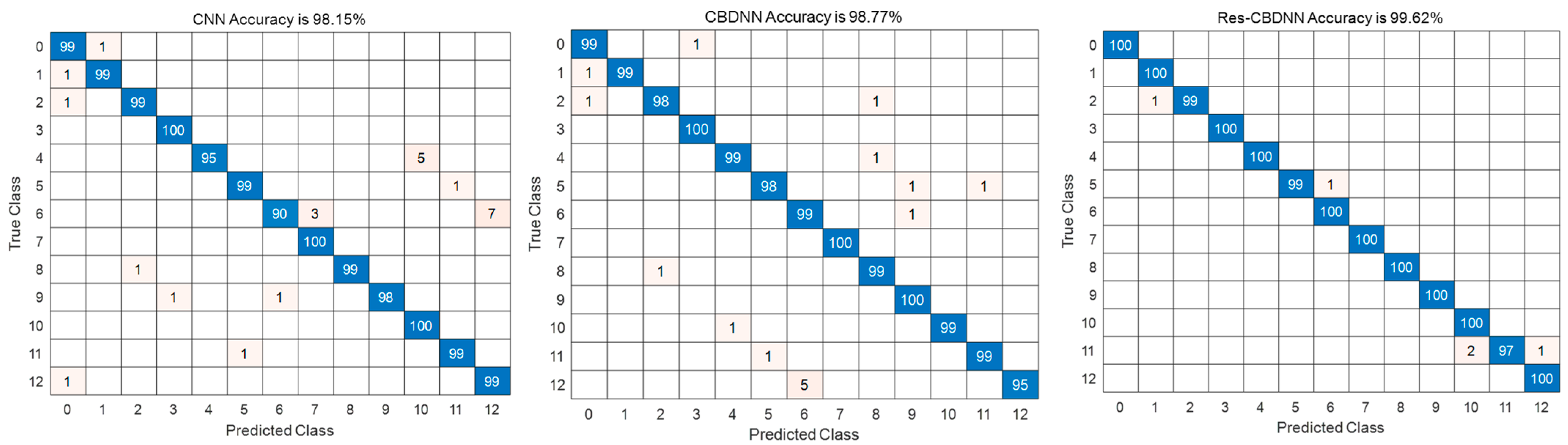
We trained the three networks using 10,400 simulated data as training sets from Section 4.1; concerning the training speed, accuracy, and loss, this method is superior to the other two methods. The training accuracy rate increases most rapidly and gradually stabilizes above 95%. To avoid over-fitting, every training session would use dropout layers to remove some features. The training accuracy averages 99.62%, the loss function minimum is 0.0546, and the effect is highest. It is shown that the Res-CBDNN model has acquired abundant fault features through ResNet in the initial training stage, and the training performance is faster and more stable by learning the fault features through BiLSTM. The three well-trained networks were tested using test set data to validate their ability to troubleshoot, and their test results with a confusion matrix are shown in Figure 12 and

Table 4. Comparison of training effects of three models.

	CNN [32]	CBDNN [33]	Res-CBDNN
Average Training Accuracy	97.5%	97.88%	98.65%
Average Training Loss	0.2088	0.0870	0.0546
Testing Accuracy	98.15%	98.77%	99.62%

.

Among them, 1–12 represents 12 different HRC fault states, and 0 indicates the health state. Combined with Figure 11 and Table 4, with the CNN’s powerful feature extraction capabilities, it is possible to obtain more fault attributes and meet diagnostic needs. The CBDNN, combined with the features of BiLSTM, can learn the time features of the data with an accuracy of 98.77%. However, due to the limitation of the depth of the network, it cannot extract more fault features and cannot identify the degree of fault. The Res-CBDNN network can improve the feature extraction ability through residual connection and combine the time features learned by BiLSTM, further improving the diagnosis effect and distinguishing the fault location and state. The test results show that the Res-CBDNN is the best in training precision and loss, and the residual network can enhance the model feature extraction ability and fault location ability. BiLSTM can further study the time information in the feature, improve the state recognition ability, and obtain better fault diagnosis results.

4.3. Verification of Robustness of the Diagnostic Model

In this paper, three additive white Gaussian noises are used to simulate different levels of noise, and the Ns value is introduced to describe the sensitivity of the model to noise. The results of the three network diagnostics are shown in

Table 5. Comparison of different models under noises.

	38 dB		35 dB		33 dB
	Accuracy	Ns	Accuracy	Ns	Accuracy	Ns
CNN [32]	90.77	7.51	80.92	17.55	73.38	23.24
CBDNN [33]	97.23	1.56	86.69	12.23	81.23	17.76
Res-CBDNN	99.08	0.54	94.77	4.87	88.33	11.28

where $\mathrm{Ns}=\frac{{\mathrm{Accurcy}}_{\mathrm{none}}-{\mathrm{Accurcy}}_{\mathrm{noise}}}{{\mathrm{Accurcy}}_{\mathrm{none}}}\times 100\%$.

From Table 5, the diagnostic accuracy of the CNN and CBDNN models decreased significantly under different noises, while the diagnostic accuracy of the Res-CBDNN model was above 85%. By observing the change in accuracy under 38 dB and 33 dB noise, it can be seen that BiLSTM can capture the time series information of fault features extracted by the CNN, and the accuracy loss of diagnosis results is reduced from 17.34% to 16%. ResNet enhances CNN’s fault extraction capability, which can extract deeper fault information for BiLSTM to learn, reducing the loss of accuracy to 10.75%. In addition, the integration of feature information and time series information helps strengthen the anti-noise ability of the diagnostic model. The test results show that the anti-noise ability of the Res-CBDNN mainly comes from the combination of the residual network and CBDNN, which makes the fault diagnosis accuracy of Res-CBDNN remain high, and the diagnosis results have a certain robustness.

The confusion matrix of the Res-CBDNN diagnostic model in different noise environments is shown in Figure 13. The model’s fault state detection and fault location capabilities are analyzed based on the indicators presented in the literature [34], and the calculation result is shown in

Table 6. Evaluation of fault location effect under different noises.

Fault Location	38 dB			35 dB
	Precision	Recall	F1 Score	Precision	Recall	F1 Score
None	100	100	100	100	100	100
A	99.5	99.5	99.5	95.6	98	96.8
B	98.5	100	99.2	97.5	98	97.7
C	99	99.9	99.5	96.1	98	97
AB	98.0	100	99	85.9	98	91.6
BC	99.5	97.5	98.5	94.1	87.5	90.6
AC	100	97.5	98.7	98.8	87	92.5
Fault Location	33 dB
	Precision		Recall		F1 Score
None	100		64		78.1
A	92		98		94.9
B	97		97.5		97.3
C	81.8		96.5		94
AB	75.8		100		86.2
BC	97		80.5		97.9
AC	97.9		70		81.6

and

Table 7. Evaluation of fault detection effect under different noises.

State Detection	38 dB			35 dB
	Precision	Recall	F1 Score	Precision	Recall	F1 Score
Health	100	100	100	100	100	100
Alert	100	100	100	99.8	100	99.9
Degradation	100	100	100	99.8	100	99.9
State Detection	33 dB
	Precision		Recall		F1 Score
Health	100		64		78
Alert	93.9		98.2		96
Degradation	98.2		99.7		98.9

.

Where precision, recall, and F1 score can be determined as Equations (7)–(9) to evaluate the diagnostic performance.

$$\mathrm{Precision}=\frac{\mathrm{True}\mathrm{Postives}}{\mathrm{True}\mathrm{Postives}+\mathrm{False}\mathrm{Postives},}$$

(7)

$$\mathrm{Recall}=\frac{\mathrm{True}\mathrm{Postives}}{\mathrm{True}\mathrm{Postives}+\mathrm{False}\mathrm{Negatives},}$$

(8)

$$\mathrm{F}1 \mathrm{Score}=\frac{2\times \mathrm{True}\mathrm{Postives}}{2\times \mathrm{True}\mathrm{Postives}+\mathrm{False}\mathrm{Postives}+\mathrm{False}\mathrm{Negatives}.}$$

(9)

Combined with the confusion matrix and two tables, we found that noise mainly affects the fault location ability, especially for AB and AC. The precision and F1 scores decrease by 5.4% and 10.9%, respectively, with the increase in noise. This is due to the high similarity of two-phase fault features; the noise has covered up part of the fault features, leading to misclassification. The noise has little influence on system state identification, and the accuracy of the two kinds of fault state identification is more than 90%, so the model has strong fault detection ability.

Compared with the CNN and CBDNN, the Res-CBDNN diagnosis model has high diagnostic accuracy and anti-noise ability and can effectively identify the fault state and fault location. Therefore, it is suitable for HRC fault diagnosis of a marine electric propulsion system.

5. Conclusions

Aiming to achieve an HRC fault diagnosis of a ship’s electric propulsion system, a diagnosis model based on ResNet and BiLSTM is proposed. Firstly, the original current data are preprocessed by the wavelet transform to extract the fault high-dimensional time-frequency information, and the CNN is used to further process the fault high-dimensional information. The residual structure can avoid the gradient vanishing problem of the deep network by direct mapping and by implementing deep CNN and deep fault feature mining. Finally, BiLSTM can obtain the fault sequence features, fault degree, and location information and complete HRC fault monitoring and diagnosis. The Res-CBDNN provides an effective representation method to extract the intrinsic characteristics of HRC fault, and the residual block transfers the gradient to a deeper level, which improves the training effect. Diagnosis results show that the accuracy and robustness can be enhanced, and the anti-noise ability of the diagnosis model can be obtained by extracting the time information from BILSTM after the wavelet fault information is deeply mined by residual error network.

The Res-CBDNN combines feature extraction and classification to improve the accuracy and robustness of diagnosis. However, there are still the following problems:

• In view of the influence of noise on fault diagnosis results, although this method has a good effect in judging the degree of fault, noise will affect the accuracy of data collection under HRC fault and confuse some similar fault features. Therefore, it is necessary to preprocess the data of more scales to obtain different frequency components in the signal in order to explore whether the information contained in different scales can bring better results;
• Compared with the traditional diagnosis method based on a mathematical model, the diagnosis model based on the deep learning method is less interpretable, so it is necessary to consider how to integrate these reliable methods into DNN fault diagnosis to improve the interpretability of diagnostic methods;
• In the field of fault diagnosis, it is difficult to obtain fault data labels, which has a negative effect on supervised learning. Unsupervised learning does not need sample labels and can generate unknown data labels by clustering methods; therefore, future research will focus on how to improve the Res-CBDNN fault diagnosis model and realize the discriminant unsupervised depth model.

References

- Ceylan, B.O.; Akyuz, E.; Arslan, O. Systems-Theoretic Accident Model and Processes (STAMP) approach to analyse socio-technical systems of ship allision in narrow waters. Ocean Eng. 2021, 239, 10980. [Google Scholar] [CrossRef]
- De La Barrera, P.M.; Bossio, J.M.; Bossio, G.R. Detection of High-Resistance Connections in Industrial Power Systems during Induction Motor Start-up. IEEE Lat. Am. Trans. 2023, 21, 54–61. [Google Scholar] [CrossRef]
- Hang, J.; Zhang, J.; Cheng, M.; Zhang, B.; Ding, S. High-Resistance Connection Detection in Permanent Magnet Synchronous Machine Using Zero-Sequence Current Component. IEEE Trans. Power Electron. 2016, 31, 4710–4719. [Google Scholar] [CrossRef]
- Hang, J.; Yan, D.; Xia, M.; Ding, S.; Wang, Q. Quantitative Fault Severity Estimation for High-Resistance Connection in PMSM Drive System. IEEE Access 2019, 7, 26855–26866. [Google Scholar] [CrossRef]
- Hu, R.; Wang, J.; Mills, A.R.; Chong, E.; Sun, Z. Detection and Classification of Turn Fault and High Resistance Connection Fault in Permanent Magnet Machines Based on Zero Sequence Voltage. IEEE Trans. Power Electron. 2020, 35, 1922–1933. [Google Scholar] [CrossRef]
- Wang, H.; Lu, S.; Qian, G.; Ding, J.; Liu, Y.; Wang, Q. A Two-Step Strategy for Online Fault Detection of High-Resistance Connection in BLDC Motor. IEEE Trans. Power Electron. 2020, 35, 3043–3053. [Google Scholar] [CrossRef]
- Mengoni, M.; Zarri, L.; Tani, A.; Gritli, Y.; Serra, G.; Filippetti, F.; Casadei, D. Online Detection of High-Resistance Connections in Multiphase Induction Machines. IEEE Trans. Power Electron. 2015, 30, 4505–4513. [Google Scholar] [CrossRef]
- Chen, H.; He, J.; Guan, X.; Demerdash, N.A.O.; El-Refaie, A.M.; Lee, C.H.T. High-Resistance Connection Diagnosis in Five-Phase PMSMs Based on the Method of Magnetic Field Pendulous Oscillation and Symmetrical Components. IEEE Trans. Ind. Electron. 2022, 69, 2288–2299. [Google Scholar] [CrossRef]
- Goncalves, P.F.C.; Cruz, S.M.A.; Mendes, A.M.S. Online Diagnostic Method for the Detection of High-Resistance Connections and Open-Phase Faults in Six-Phase PMSM Drives. IEEE Trans. Ind. Appl. 2022, 58, 345–355. [Google Scholar] [CrossRef]
- Hang, J.; Zhang, J.; Ding, S.; Huang, Y.; Wang, Q. A Model-Based Strategy with Robust Parameter Mismatch for Online HRC Diagnosis and Location in PMSM Drive System. IEEE Trans. Power Electron. 2020, 35, 10917–10929. [Google Scholar] [CrossRef]
- Xu, Z.; Din, Z.; Jiang, Y.; Cheema, K.M.; Milyani, A.H.; Alghamdi, S. High-Resistance Connection Diagnosis Considering Current Closed-Loop Effect for Permanent Magnet Machine. Front. Energy Res. 2022, 10, 933246. [Google Scholar] [CrossRef]
- de la Barrera, P.M.; Bossio, G.R.; Solsona, J.A. High-Resistance Connection Detection in Induction Motor Drives Using Signal Injection. IEEE Trans. Ind. Electron. 2014, 61, 3563–3573. [Google Scholar] [CrossRef]
- Hang, J.; Wu, H.; Ding, S.; Hua, W.; Wang, Q. A DC-Flux-Injection Method for Fault Diagnosis of High-Resistance Connection in Direct-Torque-Controlled PMSM Drive System. IEEE Trans. Power Electron. 2020, 35, 3029–3042. [Google Scholar] [CrossRef]
- Sun, J.; Li, C.; Zheng, Z.; Wang, K.; Li, Y. Online Estimation of Per-Phase Stator Resistance Based on DC-Signal Injection for Condition Monitoring in Multiphase Drives. IEEE Trans. Ind. Electron. 2022, 69, 2227–2239. [Google Scholar] [CrossRef]
- Gonzalez-Jimenez, D.; Del-Olmo, J.; Poza, J.; Garramiola, F.; Sarasola, I. Machine Learning-Based Fault Detection and Diagnosis of Faulty Power Connections of Induction Machines. Energies 2021, 14, 4886. [Google Scholar] [CrossRef]
- Allafi, I.M.; Foster, S.N. Condition Monitoring Accuracy in Inverter-Driven Permanent Magnet Synchronous Machines Based on Motor Voltage Signature Analysis. Energies 2023, 16, 1477. [Google Scholar] [CrossRef]
- Yan, H.; Peng, Y.; Shang, W.; Kong, D. Open-circuit fault diagnosis in voltage source inverter for motor drive by using deep neural network. Eng. Appl. Artif. Intell. 2023, 120, 105866. [Google Scholar] [CrossRef]
- Jia, D.; Wang, T.; Amirat, Y.; Tang, Y. An Inequality Indicator for High-Resistance Connection Fault Diagnosis in Marine Current Turbine. JMSE 2023, 11, 97. [Google Scholar] [CrossRef]
- Hoang, D.-T.; Kang, H.-J. A survey on Deep Learning based bearing fault diagnosis. Neurocomputing 2019, 335, 327–335. [Google Scholar] [CrossRef]
- Yu, C.; Qi, L.; Sun, J.; Jiang, C.; Su, J.; Shu, W. Fault Diagnosis Technology for Ship Electrical Power System. Energies 2022, 15, 1287. [Google Scholar] [CrossRef]
- Wang, M.-H.; Lu, S.-D.; Liao, R.-M. Fault Diagnosis for Power Cables Based on Convolutional Neural Network with Chaotic System and Discrete Wavelet Transform. IEEE Trans. Power Deliv. 2022, 37, 582–590. [Google Scholar] [CrossRef]
- Kim, M.; Jung, J.H.; Ko, J.U.; Kong, H.B.; Lee, J.; Youn, B.D. Direct Connection-Based Convolutional Neural Network (DC-CNN) for Fault Diagnosis of Rotor Systems. IEEE Access 2020, 8, 172043–172056. [Google Scholar] [CrossRef]
- Nacer, S.M.; Nadia, B.; Abdelghani, R.; Mohamed, B. A novel method for bearing fault diagnosis based on BiLSTM neural networks. Int. J. Adv. Manuf. Technol. 2023, 125, 1477–1492. [Google Scholar] [CrossRef]
- Meng, F.; Yang, S.; Wang, J.; Xia, L.; Liu, H. Creating Knowledge Graph of Electric Power Equipment Faults Based on BERT–BiLSTM–CRF Model. J. Electr. Eng. Technol. 2022, 17, 2507–2516. [Google Scholar] [CrossRef]
- Lu, W.; Li, J.; Wang, J.; Qin, L. A CNN-BiLSTM-AM method for stock price prediction. Neural Comput. Appl. 2021, 33, 4741–4753. [Google Scholar] [CrossRef]
- Bazi, R.; Benkedjouh, T.; Habbouche, H.; Rechak, S.; Zerhouni, N. A hybrid CNN-BiLSTM approach-based variational mode decomposition for tool wear monitoring. Int. J. Adv. Manuf. Technol. 2022, 119, 3803–3817. [Google Scholar] [CrossRef]
- Huang, T.; Zhang, Q.; Tang, X.; Zhao, S.; Lu, X. A novel fault diagnosis method based on CNN and LSTM and its application in fault diagnosis for complex systems. Artif. Intell. Rev. 2022, 55, 1289–1315. [Google Scholar] [CrossRef]
- Dibaj, A.; Ettefagh, M.M.; Hassannejad, R.; Ehghaghi, M.B. A hybrid fine-tuned VMD and CNN scheme for untrained compound fault diagnosis of rotating machinery with unequal-severity faults. Expert Syst. Appl. 2021, 167, 114094. [Google Scholar] [CrossRef]
- Yao, J.; Jiang, X.; Wang, S.; Jiang, K.; Yu, X. SVM-BiLSTM: A Fault Detection Method for the Gas Station IoT System Based on Deep Learning. IEEE Access 2020, 8, 203712–203723. [Google Scholar] [CrossRef]
- Guo, Y.; Mao, J.; Zhao, M. Rolling Bearing Fault Diagnosis Method Based on Attention CNN and BiLSTM Network. Neural Process. Lett. 2023, 55, 3377–3410. [Google Scholar] [CrossRef]
- Diao, N.; Wang, Z.; Ma, H.; Yang, W. Fault Diagnosis of Rolling Bearing Under Variable Working Conditions Based on CWT and T-ResNet. J. Vib. Eng. Technol. 2022, 11, 3747–3757. [Google Scholar] [CrossRef]
- Qian, L.; Li, B.; Chen, L. CNN-Based Feature Fusion Motor Fault Diagnosis. Electronics 2022, 11, 2746. [Google Scholar] [CrossRef]
- Bharatheedasan, K.; Maity, T.; Kumaraswamidhas, L.A.; Durairaj, M. An intelligent of fault diagnosis and predicting remaining useful life of rolling bearings based on convolutional neural network with bidirectional LSTM. Sādhanā 2023, 48, 131. [Google Scholar] [CrossRef]
- Shakiba, F.M.; Shojaee, M.; Azizi, S.M.; Zhou, M. Generalized fault diagnosis method of transmission lines using transfer learning technique. Neurocomputing 2022, 500, 556–566. [Google Scholar] [CrossRef]
Figure 1.
Structure of main power unit of an electric propulsion ship.
Figure 2.
HRC fault diagram of ship electric propulsion system.
Figure 3.
System performance of alert and degraded.
Figure 4.
Comparison of torque harmonics under different HRC fault states.
Figure 5.
Current change under different faults.
Figure 6.
Schematic diagram of BiLSTM data transmission.
Figure 7.
A diagram of the CBDNN model architecture.
Figure 8.
Residual network structure diagram.
Figure 9.
Structure of Res-CBDNN diagnostic model.
Figure 10.
Diagnostic flow chart for Res-CBDNN.
Figure 11.
Comparison of (a) the training accuracy and (b) training loss of CNN, CBDNN, and Res-CBDNN diagnostic models.
Figure 12.
Confounded matrix of diagnostic results of three models.
Figure 13.
Res-CBDNN diagnostic results of confusion matrix under different noises.