Integrating Machine Learning and MLOps for Wind Energy Forecasting: A Comparative Analysis and Optimization Study on Türkiye’s Wind Data

Abstract

This study conducted a detailed comparative analysis of various machine learning models to enhance wind energy forecasts, including linear regression, decision tree, random forest, gradient boosting machine, XGBoost, LightGBM, and CatBoost. Furthermore, it developed an end-to-end MLOps pipeline leveraging SCADA data from a wind turbine in Türkiye. This research not only compared models using the RMSE metric for selection and optimization but also explored in detail the impact of integrating machine learning with MLOps on the precision of energy production forecasts. It investigated the suitability and efficiency of ML models in predicting wind energy with MLOps integration. The study explored ways to improve LightGBM algorithm performance through hyperparameter tuning and Docker utilization. It also highlighted challenges in speeding up MLOps development and deployment processes. Model performance was assessed using the RMSE metric, conducting a comparative evaluation across different models. The findings revealed that the RMSE values among the regression models ranged from 460 kW to 192 kW. Focusing on enhancing LightGBM, the research decreased the RMSE value to 190.34 kW. Despite facing technical and operational hurdles, the implementation of MLOps was proven to enhance the speed (latency of 9 ms), reliability (through Docker encapsulation), and scalability (using Docker swarm) of machine learning endeavors.

1. Introduction

Wind energy has gained increasing importance in electrical energy production in recent years and has become an indispensable part of the sustainable energy portfolio. This technology transforms wind mechanical energy to electrical energy using wind turbine subsystems. It stands out as a solution for the future of energy production because it is environmentally friendly, offers an unlimited resource, and keeps carbon emissions to a minimum. Wind energy production offers great advantages in environmental protection thanks to the use of a clean and renewable resource. This renewable source decreases CO₂ emissions and makes better environmental impact of the energy plants, especially in terms of air quality. Thus, it plays an effective role in combating climate change. In addition, the installation of wind power plants prevents environmental destruction and minimizes the negative effects on ecosystems.

Türkiye is very advantageous in terms of wind energy potential. There is a potential of 47.849,44 MW, especially in the regions where the Renewable Energy Resource Area (YEKA) has been declared [1]. Wind farms in these regions make significant contributions to economic development as well as increasing national energy security. Wind turbines are designed to convert wind energy, which has kinetic energy, first into mechanical energy and then into electrical energy [2]. Uninterrupted and strong wind speeds are required for effective electricity generation; however, wind speed variability is a significant challenge for electricity generation. In order to solve this problem, it is necessary to make short-term wind speed forecasts. These predictions are used to optimize energy production, prevent damage to turbines and equipment, and ensure a safe operating environment. Short-term wind speed forecasts are made by analyzing meteorological data. These predictions are critical for adjusting turbines’ operating speeds and heights, maximizing energy production, and ensuring facility safety. The accuracy of these predictions plays a vital role in the efficiency and sustainability of wind energy facilities.

The concept of machine learning operations (MLOps) has emerged through the integration of machine learning (ML) applications with DevOps-based software development processes. MLOps involves the development and maintenance of ML models, incorporating continuous integration to deliver efficient and dependable service [3]. Professionals from various fields, including data scientists, DevOps engineers, and software experts, collaborate in this endeavor. The primary goal of MLOps is to ensure the effective and efficient production of software, as well as to support ML-based software development [4]. However, the reliance on multiple project management tools can create bottlenecks in MLOps. Effective delegation of tasks and communication among teams is crucial due to the collaborative nature of the process. Therefore, MLOps environments should be equipped with a diverse array of tools to facilitate these interactions [5]. In an MLOps environment that emphasizes frequent changes to the source model, achieving automatic traceability across diverse software artifacts following a thorough Change Impact Analysis (CIA) and Change Propagation (CP) can be challenging [6].

In the field of software engineering, different software process models and development methodologies have emerged over time. Methodologies such as waterfall and agile methods aim to deliver production-ready software products [7]. The concept of DevOps, which emerged in 2008/2009, aims to reduce problems in software development and represents more than a methodology. It emphasizes collaboration, communication, and information sharing, eliminating the gap between development and operations [8]. DevOps promotes continuous integration, delivery, and deployment, while also including practices such as continuous testing, quality assurance, and monitoring. This new approach requires developers to not only develop software but also care about running it [9]. DevOps ensures better software quality and facilitates the successful integration of ML models into live environments [10,11]. This study highlights the importance of integrating an ML model developed for wind energy forecasting into the MLOps process. The research aims to detail the processes of MLOps approaches for data exploration, experimental monitoring, and model deployment and management. This work is an important step in overcoming current barriers to implementing ML models into live implementation and providing guidance to data scientists and software engineers.

The main purpose of the research is to examine how to successfully develop an ML model, how to effectively take it into the live environment, and what support the methodology and tools offered by MLOps can provide in this process. In this context, the focus of the research is a detailed examination of MLOps approaches, covering stages such as data analysis, experimental monitoring of wind energy forecast models, model deployment, and model management throughout the controlled model development process. The study addresses the factors that prevent the successful integration of ML models into live environments and guides data scientists and software engineers on how to turn the developed ML models into applications using MLOps approaches.

The paper is organized in the following manner. Section 2 provides an overview of the literature pertaining to wind energy and ML, as the integration of these two ideas forms the foundation of the MLOps technological framework. Following this, Section 3 outlines the materials and methods utilized in the study. Moreover, a pipeline design of MLOps is described in Section 4. Experimental results for the obtained and targeted outputs are given in Section 5. Section 6, which is a discussion, and Section 7, which presents the conclusion and future works, conclude the proposed idea with suggestions and possible future research directions for wind energy-based MLOps.

2. Literature Background

Proposed models for wind energy prediction can be categorized as physical models, traditional statistical models, ML models, and other hybrid models [12]. In 2023, Li et al. proposed a theoretical model of an integrated system based on a conical Concrete-Filled Double Skin Tube (CFDST) wind turbine, aiming to investigate the dynamic behavior of the integrated system in the field of wind energy. A model was formulated utilizing the Lagrangian approach for the governing equation, and it was analytically solved through the Galerkin method. The developed model was validated with wind tunnel tests of scaled models, followed by extensive parametric discussions. This study resulted in a reliable analytical model capable of accurately predicting the fundamental frequency and displacement response, which has been corroborated [13].

Unlike physical models, statistical models use meteorological information to estimate wind speed and include a Numerical Weather Prediction (NWP) model to estimate wind speed [14,15]. The Weather Research Forecast (WRF) model, which considers the intricacies of the terrain and the resolution of the chosen region, is also employed as an effective forecasting method for predicting wind speed. It has demonstrated favorable performance in short-term wind speed prediction [16].

The autoregressive integrated moving average (ARIMA) model is the most used traditional statistical model. It utilizes historical data to create a prediction model that effectively captures the linear relationship within the training dataset [14]. As statistical models and synthetic techniques have advanced, ML models have been introduced to enhance prediction models [17]. ML-based models, including artificial neural networks (ANNs), fuzzy logic (FL) methods, and support vector machines (SVMs), are extensively employed in wind speed prediction [16]. However, it is important to note that no single method is universally applicable to all datasets [18]. Consequently, hybrid models that combine traditional statistical models with ML models have been proposed to enhance the accuracy of wind speed prediction [12]. Numerous studies have focused on integrating individual prediction models to create improved prediction models. Nevertheless, a review of wind speed estimation studies has revealed a lack of universally accepted definitions for these approaches [12]. Additionally, there are other prediction models that combine different prediction methods, such as hybrid approaches that incorporate parameter optimization, dataset preprocessing techniques, and error handling techniques [18].

ML algorithms are designed to identify patterns and correlations within extensive datasets, enabling them to make optimal decisions and predictions through thorough analysis [19]. As machine learning applications gain access to larger volumes of data, their performance improves, and they become increasingly successful. These algorithms utilize the framework of regression analysis techniques to construct prediction models and determine the associations between variables [20]. Linear regression (LR) is a supervised learning algorithm in machine learning that predicts the value of a variable based on another variable. It utilizes LR calculators with the least squares method to determine the best-fit line for a set of paired data [21]. On the other hand, random forest (RF) regression improves prediction accuracy by utilizing the decision tree (DT) method multiple times, with decision trees being randomly selected subsets from the dataset [22]. XGBoost regression is a successful method based on the eXtreme Gradient Boosting decision tree algorithm [23]. Since eXtreme Gradient Boosting (XGBoost) uses the parallel working technique when revealing the decision tree, operations occur quickly. One of its most well-known and important capabilities is that it can use the observation point in the dataset according to its weight values to find the appropriate point when classifying data into many trees.

LightGBM, the Light Gradient Acceleration Machines technique, has a histogram-based infrastructure [24]. In the LightGBM method, the training time of the decision tree has a non-inverse proportion to the resulting calculation and subsequent division. As a result of this ability, training time is not long and resource usage is reduced. LightGBM grows trees leaf-wise rather than level-wise and can handle large-sized data with a significant reduction in training time [25]. Similar to XGBoost, LightGBM can be applied to wind turbine data to predict power output or detect potential faults. Its efficient processing of large datasets makes it suitable for processing high volumes of data typically generated by wind turbines. CatBoost, on the other hand, is an algorithm for gradient boosting in decision trees that is particularly powerful in dealing effectively with categorical features. CatBoost can be used when wind turbine datasets have a large number of categorical features, such as turbine models, locations, or operating modes. The ability to naturally process categorical data can simplify preprocessing steps [25].

ML models were developed for wind energy as part of the study. However, the study also focused on transforming these ML models into real-life applications. To achieve this, various research analyses were conducted to explore the potential applications and emerging trends of MLOps studies. Successful data science projects require the collaboration of different business layers. Some researchers emphasize the importance of continuous delivery of MLOps and the automation of various stages of the machine learning workflow [26]. Additionally, data science projects drive the development of hardware capabilities to enhance computing power and energy efficiency [27]. As a result, there is a growing interest within the research community in networking for MLOps [28]. Function-As-A-Service (FaaS) technologies are considered enablers of MLOps models, and deploying pre-trained ML models on FaaS can unlock the potential of event-driven AI solutions [29]. Constant monitoring is essential for ML-based applications to ensure reliable performance in critical systems. Lastly, traditional version control systems used in software engineering often struggle to differentiate between machine learning-specific components like models and datasets. Further research is needed in this area to better support the machine learning life cycle [30].

3. Material and Methods

In this section, the materials, datasets, software tools, and methodological approaches used for the integration of the ML model developed for wind energy forecasting into the MLOps process are explained in detail. By specifying the source, features, and preprocessing steps of the datasets used in the research, the basis for training the model is laid.

3.1. Dataset and Preprocessing

The dataset used in this study includes data recorded at 10 min intervals from the Supervisory Control and Data Acquisition (SCADA) system of an operating wind turbine in Türkiye [31]. Features in the dataset are as follows: LV (Low Voltage) Actual Power (kW), which expresses the power produced by the turbine for a certain moment; Wind Speed (m/s), which shows the wind speed used by the turbine for electricity production; Theoretical Power Curve (KWh), which expresses the theoretical power values for that wind speed specified by the turbine manufacturer; and Wind Direction (°), which shows the wind direction in which the turbine automatically rotates. Sample data from the dataset are given in

Table 1. Sample data in the dataset.

Index	Date	Actual Power (kW)	Wind Speed (m/s)	Thpower (KWh)	Wind Direction (°)
0	1 January 2018 00:00	380.047791	5.311336	416.328908	259.994904
1	1 January 2018 00:10	453.769196	5.672167	519.917511	268.641113
2	1 January 2018 00:20	306.376587	5.216037	390.900016	272.564789

.

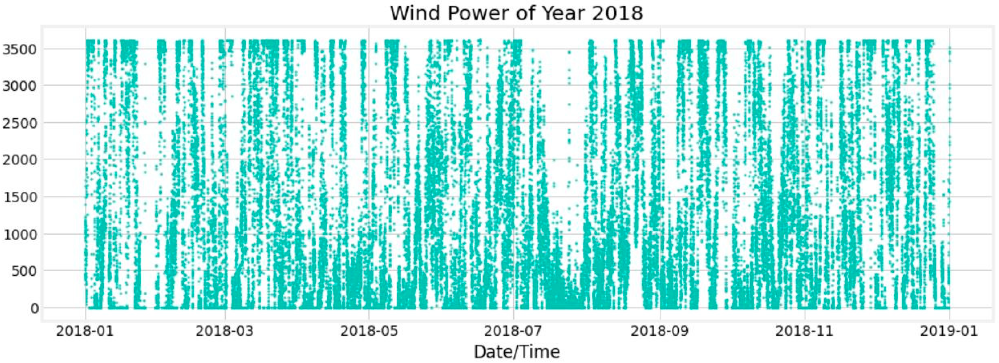
In Table 1, each row represents values over a period of time recorded at 10 min intervals. ‘Thpower (KWh)’ represents the Theoretical Power Curve. How the wind speed, and therefore the production capacity, of the wind turbine change over time is given in Figure 1.

As seen in Figure 1, it is possible to observe that on some dates, energy production is almost zero, while at other times it is very close to maximum capacity. These fluctuations reflect the natural variability of wind and the difficulties in predicting wind energy production. A correlation heatmap graph was obtained to show the strength and direction of the relationship between the variables in the dataset (Figure 2). Correlation is a statistical metric that quantifies the strength and direction of the association between two variables. The visualization process commences with the application of the ‘df.corr()’ method, which calculates the Pearson correlation coefficients within the dataset. This computation yields a correlation matrix, delineating the correlation coefficients for every possible pair of variables contained within the dataset. To visualize this matrix, the ‘heatmap’ function from the seaborn library, a data visualization library that extends ‘matplotlib’, is utilized. ‘Seaborn’ facilitates the creation of graphs that are not only more aesthetically pleasing but also more comprehensible.

The graph presented in Figure 2 is a correlation heatmap generated from a dataset comprising wind energy metrics pertinent to this investigation. The heatmap essentially functions as a matrix that visually encodes the correlation coefficients between disparate data columns through a spectrum of colors. The color intensity on the heatmap indicates the strength of the correlation between pairs of variables: hues approaching dark red signify positive correlations, whereas those approaching dark blue denote negative correlations. The values of correlation coefficients range from −1 t −o +1, where +1 signifies a perfect positive linear relationship, −1 signifies a perfect negative linear relationship, and 0 indicates no linear relationship exists [19].

Within the context of this study, the variables ‘Actualpower’, ‘Windspeed’, ‘Thpower’, and ‘Winddir’ are considered. ‘Actualpower’ and ‘Thpower’ denote the wind energy production values; ‘Windspeed’ is indicative of wind velocity; and ‘Winddir’ signifies the direction of the wind. The heatmap delineates both the magnitude and direction of the linear correlations among these variables. Notably, there exists a pronounced positive correlation amongst ‘Actualpower’, ‘Windspeed’, and ‘Thpower’, which implies robust positive linear interrelations between these variables. ‘Thpower’, or the Theoretical Power Curve, elucidates the maximum power generation potential of wind turbines under ideal conditions. However, actual conditions or the specific focus of this study may deviate from these theoretical estimations. Consequently, if the analysis is concentrated on the actual energy yield, incorporating theoretical values could potentially lead to misconceptions. Therefore, such theoretical values were omitted from this research. Subsequently, the dataset was refined to omit records wherein wind speed was between 3 and 26 m/s and the corresponding ‘LV ActivePower’ was recorded as 0 kW. The refined dataset is portrayed in a matrix combining scatter plots and histograms, as depicted in Figure 3.

Figure 3 shows the positive relationship between Wind Speed and Actual Power. There is no clear relationship between Wind Speed and Wind Direction. However, it can provide important information for applications such as choosing appropriate locations for wind turbines, energy production forecasts, and adjusting the direction of the turbine. For this reason, the wind rose graph is given in Figure 4.

Figure 4 shows the direction (in degrees) and speed (in meters/seconds) of the wind. The wind vane has sections extending outward from the center, indicated by different colors for different wind speeds. Each slice represents the frequency and speed at which the wind blows from that direction. Figure 4 shows that the wind blows most frequently from the northeast (N-E) and southeast (S-E). The highest wind speeds (e.g., over 20.2 m/s) were observed in northeasterly winds.

3.2. Feature Engineering and Data Cleaning

Machine learning models perform better when trained on representative examples from the dataset. For this reason, it is aimed for the model to learn the real relationship between wind speed and energy production by removing zero power records that disrupt the relationship between energy production and wind speed. Likewise, there may be records where the wind speed is sufficient for energy production but the turbine does not produce active power. These records must be removed. Therefore, when $W$ represents the wind speed, data were removed from the dataset according to the condition $W\le 3\left|\right|W\ge 26$.

The ‘Date/Time’ column in the dataset was processed to reveal important information that will contribute to time series analysis. Time units such as year, month, day, hour, and minute were separated in detail, thus making it possible to comprehensively examine time-related patterns. Additionally, categorical variables such as ‘Season’ and ‘Day’ were added to integrate seasonal effects and various time periods of the day into the models. However, before this stage, ‘NULL’ data were removed from the dataset. A total of 47,033 data were used in the dataset; 80% of the data in the dataset was reserved for training and 20% for testing.

3.3. Machine Learning Model Descriptions

The application of machine learning models is of strategic importance in wind energy forecasting. However, the data must be processed correctly. In this context, the dataset was examined using advanced analytical techniques and a series of regression models were evaluated for their ability to predict wind turbine active power production data. Each model was examined and compared in terms of various aspects such as predictive accuracy, computational efficiency, and ease of use.

3.3.1. Linear Regression

Distinguished by its simplicity and widespread application, linear regression is important for predictive analytics. Its ability to distinguish relationships between dependent and independent variables and to make continuous variable projections leads to its widespread use. It is developed by estimating the linear relationship between one or more variables and often using the least squares method for optimization [32].

3.3.2. Decision Tree and Random Forest

Decision trees are a modeling technique used in classification and regression problems and are widely preferred in the fields of data mining and machine learning [33]. A decision tree is a hierarchical structure that represents a dataset and consists of a set of decision rules. The purpose of this structure is to separate the samples in the dataset into classes using simple decision structures. While creating the decision tree, the feature that best divides the dataset is selected at each node. Starting from the root of the tree, each branch classifies the data or makes regression predictions until the last leaf nodes. Advantages of decision trees include the ease of understanding of the model, the low need for data preprocessing, and the ability to work with both numerical and categorical data. However, decision trees can be prone to overfitting; this is when the model fits the training data very well but performs poorly on new, unseen data [25].

Random forest (RF) is a powerful machine learning algorithm based on combining predictions produced by multiple decision trees, used for classification and regression problems [33]. By combining the predictions made by decision trees, RF minimizes the overfitting problem that a single decision tree may encounter and generally produces more stable results. This method, developed by Leo Breiman in 2001, is based on the principle of training each decision tree on randomly selected subsets and thus increases the diversity and robustness of the model. Random forests are preferred in many application areas, thanks to their capacity to determine the importance of variables, especially in high-dimensional datasets. The success of this method can be further increased by the appropriate selection of the number of variables and number of trees depending on the size and complexity of the dataset.

3.3.3. Gradient Boosting Machines

Gradient boosting machines (GBMs) represent a class of highly efficient and flexible machine learning algorithms known for their ability to solve a variety of predictive modeling problems [23]. GBMs improve prediction accuracy by iteratively combining multiple weak models, usually decision trees, into a robust ensemble estimator. GBMs are adaptively tuned to minimize a given loss function by leveraging gradient descent optimization in the function space. This feature makes them applicable in a wide variety of tasks with different data distributions and levels of complexity. The working principle of a GBM is shown in Equation (1).

$$F_m\left(x\right)=F_{m-1}\left(x\right)+p_m{h}_m\left(X\right)$$

(1)

In Equation (1), $F_m\left(x\right)$ is $m$-th iteration model forecast, $F_{m-1}\left(x\right)$ is the prediction from the previous iteration, $h_m\left(x\right)$ is a weak learner added in the current iteration (usually a decision tree), and $p_m$ is the coefficient that measures the weak learner’s contribution. A GBM learns patterns and complexities in the dataset step by step. At each step, it adds a new weak learner that will reduce the model’s previous errors. This process continues iteratively to minimize a specified loss function. Thus, the overall prediction performance of the model increases throughout the iterations.

3.3.4. XGBoost

XGBoost, an application of GBM, stands out because of its efficiency and performance, especially when working with complex and high-dimensional data. The structure of the model allows the integration of multiple weak predictors to create a robust final model that can address a variety of predictive modeling challenges. XGBoost uses both linear and tree learning algorithms to improve prediction accuracy [23]. Due to its adaptability and scalability, this technique has been chosen to tackle the complex problem of potential wind energy estimation.

The XGBoost algorithm is an advanced ensemble tree method that produces predictions using a large number of multiple regression trees. The basic step of the algorithm is to make the first prediction (base score); this is usually accomplished with a default initial value of 0.5. This value provides an iterative convergence towards the result with the improvements made in the next steps of the algorithm. By following the gradient boosting methodology, XGBoost adds a new decision tree to minimize existing errors in each iteration. In this process, each decision tree is constructed to learn the deviations (residuals) from previous predictions. These residuals are calculated as the difference between the actual values and the model’s predictions. The power of the algorithm lies in the fact that the sum of these weak learners can form a strong overall model by systematically reducing errors. In XGBoost, the branching of each decision tree is performed by optimization to minimize a customized objective function [34].

3.3.5. LightGBM

Light Gradient Boosting Machine (LightGBM) is a machine learning algorithm built on the gradient boosting framework. LightGBM is known for offering high efficiency and speed, low memory usage, and high accuracy rates on large datasets. Unlike traditional gradient boosting methods, instead of randomly selecting samples in the dataset, LightGBM processes the data using innovative techniques such as gradient-based one-sided sampling (GOSS) and exclusive feature bundling (EFB). These strategies significantly reduced the computational load and memory usage, making LightGBM widely used in energy forecasting systems [25].

3.3.6. CatBoost

The CatBoost algorithm integrates gradient boosting decision tree (GBDT) technology with advances in the effective use of categorical features. This approach improves the model’s ability to efficiently process and learn categorical data without the need for extensive preprocessing. CatBoost uses unregistered trees, which contributes to its high performance and accuracy by simplifying the handling of categorical variables. This methodology significantly helps in minimizing overfitting and thus improves the generalization capabilities of the model. CatBoost can be applied to both regression and classification problems and shows particularly high performance on large datasets. One of the main advantages of the algorithm is that it can use categorical variables directly without requiring preprocessing, which simplifies and speeds up the modeling process [25].

CatBoost works by creating a set of decision trees that are weighted to reduce the prediction error of the target variable at each step. Before adding each tree, the model randomly selects a subset of the dataset and performs gradient calculations for each element in that subset. These gradients determine how new trees are created, helping the model reduce its error rate. Additionally, CatBoost has the ability to calculate the importance of each feature, which allows the model to make more accurate predictions.

4. MLOps Pipeline Design

In this study, MLOps was used to integrate machine learning models into the software development process. A methodology leveraging DevOps practices was implemented to effectively automate and monitor ML models in the development environment. The study highlighted the key components of the MLOps development process, including model design and training data editing, and discusses how MLOps facilitates more accessible, faster, and less risky software development. The need for technical automation is outlined to drive continuous development phases and thus increase productivity through rapid model building, high-quality machine learning models, and rapid deployment.

4.1. MLOps Pipeline Architecture

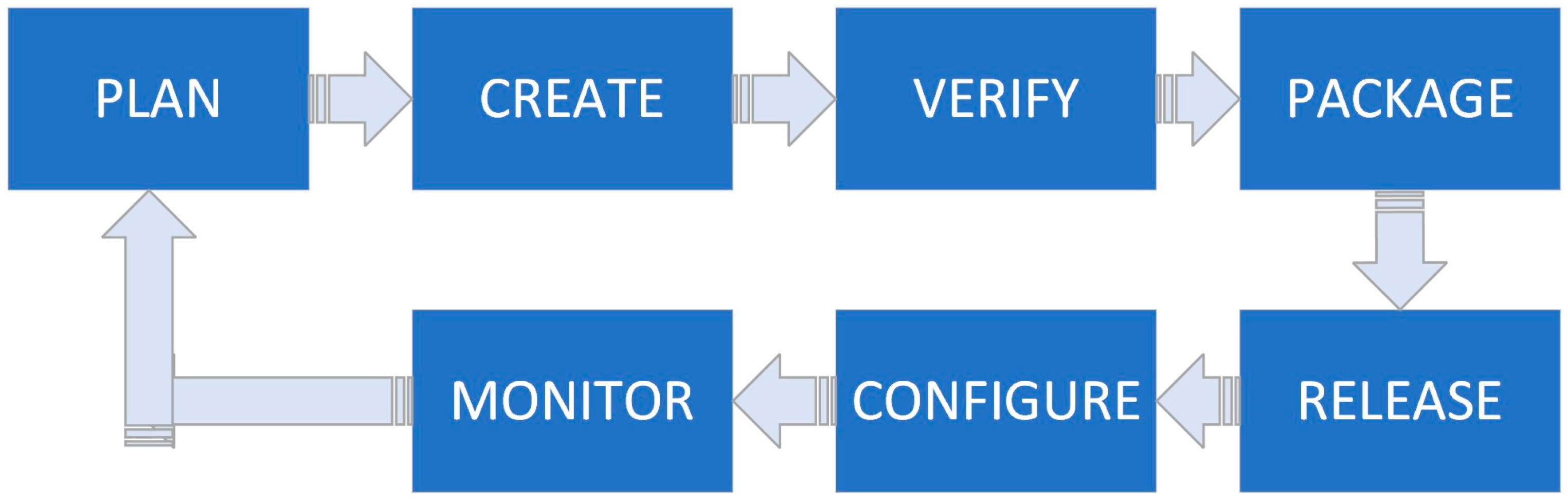
Model deployment, which involves running, scaling, maintaining, and integrating models into applications, remains a significant challenge across different industries. This process is crucial to transforming ML models into operational solutions that can drive real-world applications and outcomes. Successful deployment of models requires a robust infrastructure that can handle the computational demands of machine learning algorithms, as well as continuous monitoring and updates to ensure models remain effective over time. The MLOps pipeline architecture is a structure that automates the development, testing, deployment, and monitoring processes of machine learning projects. This architecture includes basic components such as data preparation, model training, model evaluation, model deployment, and continuous monitoring of the model’s performance. Similarly, DevOps represents a significant transformation in software development over the last decade. The DevOps approach aims to deliver software products and features faster and more reliably. The DevOps process generally includes planning, development, testing, packaging, deployment, configuration, and monitoring steps. The DevOps architecture is given in Figure 5.

When the architecture in Figure 5 is examined, it is seen that it represents a constantly renewed and active working process. The depicted architecture in Figure 5 epitomizes the structured progression of the DevOps pipeline, elucidating the systematic sequence of operations from conception to deployment. It commences with the ‘Plan’ phase, wherein strategic initiatives are formulated, encompassing requirement elicitation and delineation of developmental trajectory. This is succeeded by the ‘Create’ phase, where the amalgamation of coding practices comes to fruition through collaborative and iterative development. After the creation phase is ‘Verify’, a critical juncture wherein the developed features undergo rigorous automated validation to ensure adherence to predefined quality benchmarks and functional integrity. Upon successful verification, the ‘Package’ phase ensues, entailing the encapsulation of validated features into deployable entities, primed for integration into the user environment. The ‘Release’ phase marks the deployment of the application into the production milieu, orchestrated to minimize manual intervention and foster seamless operational continuity. This is closely followed by the ‘Configure’ phase, which involves the meticulous tuning of the application within its deployment ecosystem to ensure optimal performance parameters are met. Crucially, the ‘Monitor’ phase encapsulates the ongoing surveillance of application performance post-deployment, serving as a feedback conduit to the ‘Plan’ phase, thereby instituting a cyclical paradigm of continuous enhancement and evolution. This feedback mechanism is pivotal, facilitating empirical insights that drive the iterative refinement of the subsequent developmental iterations.

Different technologies can be used at each step of the DevOps architecture. DevOps can use tools like JIRA for planning, Git and IDEs for code generation, Docker for packaging, Jenkins for deployment, and Prometheus/Grafana for monitoring. Flexibility here may vary depending on the developer’s current hardware requirements. Just as DevOps has introduced new approaches to software development, MLOps has brought a similar transformation to ML operations. Although progress has been made in integrating ML into different applications and technological products, a solid structure is needed to ensure fast and reliable delivery of ML products. Therefore, ML needs to be operationalized. 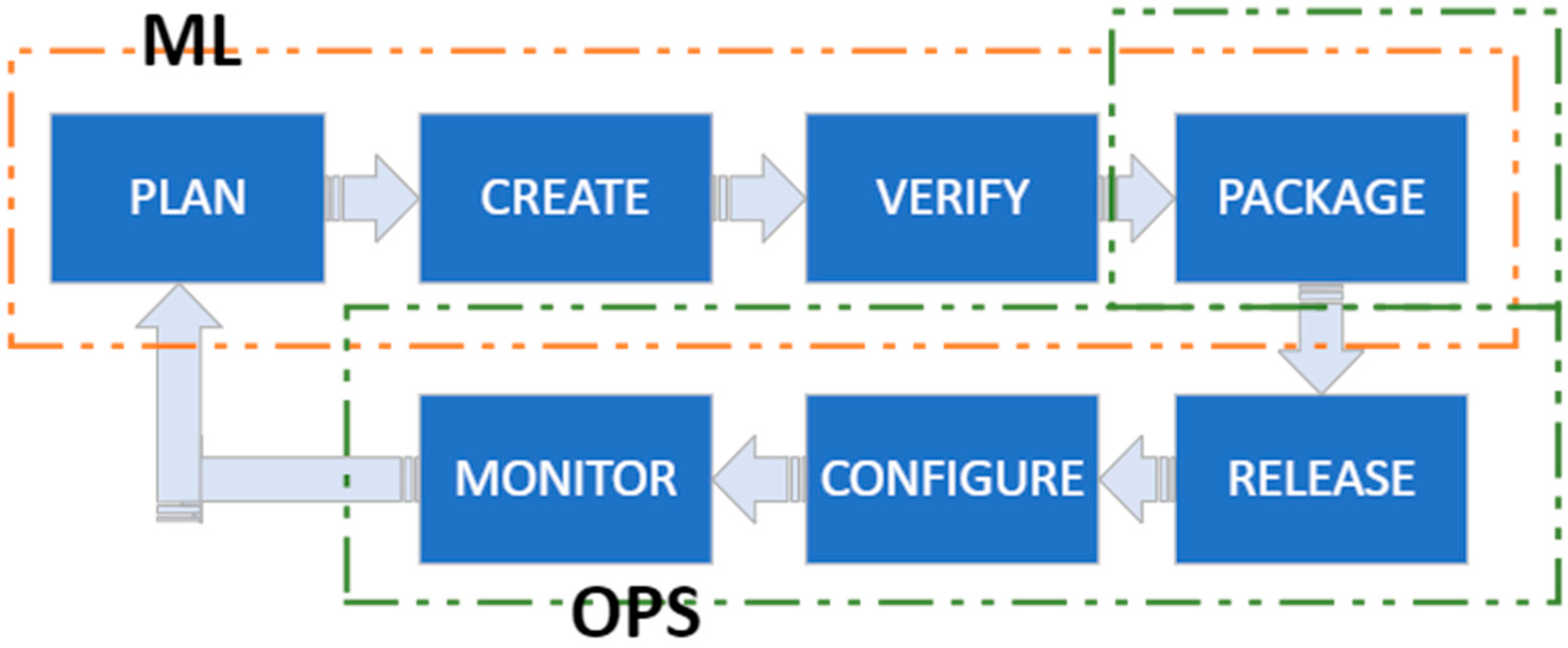Figure 6 shows the MLOps architecture inspired by DevOps.

The adaptation of DevOps processes to the MLOps process aims to meet the unique needs of ML using open-source technologies. This process covers the life cycle stages of ML models such as data preparation, model training, model versioning, deployment, and monitoring. With this adaptation, ML models are managed at the same level as the software development discipline, ensuring seamless integration into products and services. The ‘CREATE’ phase shows the development phase where the code of the product is written. In the MLOps process, relevant ML models are created using libraries such as TensorFlow and Keras, with the help of any editor such as Jupyter. In this study, ML models were developed using Jupyter and Python’s sklearn library. The ‘VERIFY’ step refers to the quality control processes where code is tested and verified. At this stage, the accuracy of ML models was tested using metrics such as root mean squared error (RMSE). The ‘PACKAGE’ phase is the part where the software is packaged for distribution. In this study, docker was used for package processing. In the ‘CONFIGURE’ phase, web services were prepared to enable ML models to work in different systems. The ‘MONITOR’ phase includes the process of monitoring the performance of the software in the production environment and detecting potential problems. Although at this stage Postman is primarily a tool used for the development and testing of application programming interfaces (APIs), it has been used to test the health and response times of APIs.

4.2. Model Training and Evaluation Process

Within the framework of MLOps, model training and evaluation processes include steps such as training the model on data, testing its performance, and adjusting hyperparameters. The training process of various machine learning models for ‘LV ActivePower (kW)’ prediction based on SCADA data was carried out. The process started with the preparation of the data and dividing the data into training and test sets. Models were developed by defining various regression models in a pipeline, including LR, DT, RF, GBM, XGBoost, LightGBM, and CatBoost. RMSE was used as the evaluation criterion for each model.

Models were developed using the sklearn library in Python’s scikit-learn library. LinearRegression works by fitting a linear model with coefficients to minimize the residual sum of squares between the observed targets in the dataset and the targets predicted by the linear approximation. The model then calculates the best-fitting coefficients for the features that provide a best-fit line for the data. In the RF model, multiple decision trees are created and combined to obtain a more accurate and stable prediction. In GBR, a model is created on a stage-by-stage basis, like other strengthening methods. However, its generalization is achieved by allowing the optimization of a differentiable loss function. Model training was carried out by adding trees sequentially, each correcting the errors made by the previously trained trees.

4.3. Automatic Model Deployment and Update

Automated model deployment and update is a process that automates the integration of machine learning models into production environments and the management of updates to these models. Tools that can be used in the automatic model deployment and update phase include continuous integration and continuous deployment (CI/CD) tools such as Jenkins, Spinnaker, ad Argo CD. There are container management systems such as Kubernetes and Docker, and platforms that offer machine learning-specific features such as MLflow and TFX (TensorFlow Extended). These tools enable the model to be seamlessly integrated into the live environment, monitor its performance, and make automatic updates when necessary.

During the automatic model deployment and update phase, Docker ensures that models are packaged in containers and run consistently and isolated in any environment. This process starts by using a structure in the Dockerfile where the application and its dependencies are defined. A Docker image is created and can be stored in registries such as Docker Hub. Then, using the created image, containers are quickly deployed and run in the production environment or development and test environments. This method ensures the consistency and portability of the application across different environments. Figure 7 shows the Docker architecture used in the model distribution structure used in this study.

In the architecture shown in Figure 7, hardware with an i7 processor and 16 GB RAM capacity was used as the infrastructure. Windows 10 was preferred as the operating system. In the Docker container engine section, a structured container containing dependencies for artificial intelligence models was created. Libraries such as NumPy and scikit-learn were defined as requirements. Efficient use and sharing of resources are ensured without requiring separate operating systems. Thanks to the container engine, system resources are effectively shared through the Docker engine while applications are run in isolated environments. This approach contributed to speeding up deployment and increasing application consistency. In the APP section, an API was developed using the FastAPI library. API requests trigger the base model in the container engine section. When the base model Docker is first started up, it is loaded into memory and stands ready for API requests.

5. Experimental Results

In this study, the effectiveness of analyses and machine learning models in estimating wind energy production and managing supply in the energy market was examined. It details how model training and automatic deployment processes can be optimized with the use of Docker, MLOps tools, and various machine learning algorithms. The performance of the developed models, their accuracy in energy production forecasts, and their contribution to market supply planning were evaluated.

5.1. Model Performance and Evaluation

RMSE as a metric in the experimental results section serves to assess the accuracy of statistical forecasts made by the developed models. RMSE calculates the square root of the average of the squared differences between predicted and actual values. This measure is critical for evaluating how closely the model’s predictions match the real-world data, providing insight into the model’s predictive performance and its applicability for energy production forecasting and market supply planning.

$$RMSE=\sqrt{\sum _{i=1}^n\frac{{({\mathrm{â}}_i-a_i)}^2}{n}}$$

(2)

When evaluating a developed model using RMSE, a lower value is desirable, indicating closer alignment between predictions and actual values. Conversely, a high RMSE suggests significant discrepancies, signaling poor model performance. Thus, lower RMSE values denote more accurate predictions, reflecting better model effectiveness.

5.2. Model Comparison Using RMSE

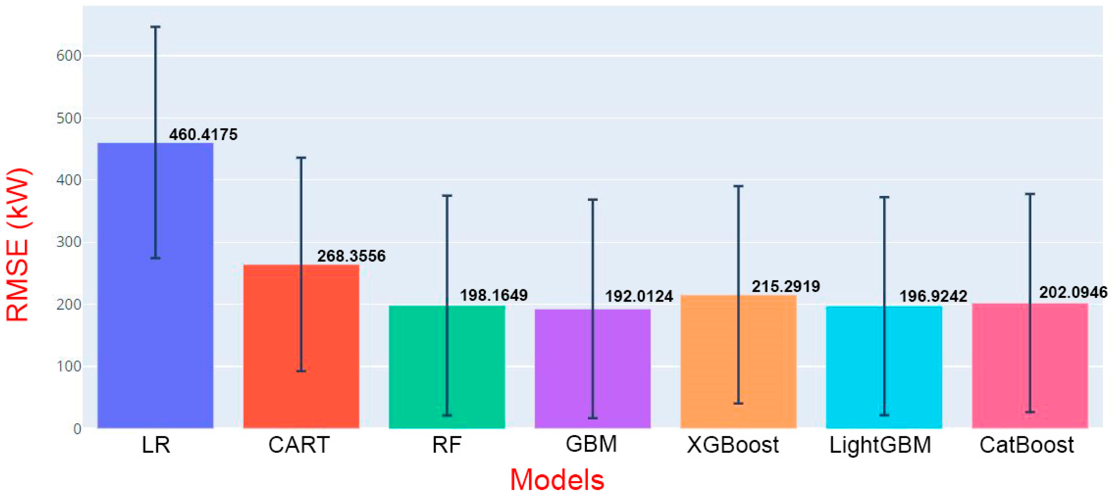
A comparative analysis of various machine learning models was performed using RMSE. In the analysis, the models developed within the scope of the study were discussed. RMSE scores of each model show the performance of the model on the dataset. Model comparisons will help determine how well models work on different datasets and in what situations they may be preferred. Figure 8 shows the graph comparing the results. Moreover, error bars representing the 95% confidence intervals have been incorporated into the bar charts that display the average error metrics for each machine learning model. This enhancement provides critical insights into the statistical reliability of the performance measures across models.

The comparisons in Figure 8 are expected to guide important decisions at the model selection stage and play a critical role in achieving success in machine learning applications. As seen in the graph, while the LR model has the highest RMSE value, the GBM model has the lowest RMSE value among these models. It is seen that the linear regression model predicts the dataset the worst compared to other models, while the GBM model has the best prediction performance among these models. However, it is observed that LightGBM and RF models perform well with similar low RMSE values. In line with these observations, LightGBM was reconsidered, and the model was improved. In addition, the RMSE values of the XGBoost and CatBoost models are close to each other, and it can be said that they exhibit a moderate performance compared to other advanced models.

5.3. LightGBM Hyperparameter Optimisation

An ideal model should make predictions with high accuracy and produce results as close as possible to the real values. Based on RMSE values, the best performers among the examined models are discussed in detail. In this context, it is discussed in detail that LightGBM performs well among the models examined, based on its RMSE values. Important points such as the advantages and limitations of LightGBM, the cases in which these models should be preferred, and the relationship between the characteristics of the dataset and model performance are emphasized. A regression model was created using the LightGBM algorithm, and cross-validation and hyperparameter tuning of this model were performed.

Hyperparameter optimization was performed using GridSearchCV. The aim is to find the combination that gives the best performance by trying different combinations of the specified parameters, including ‘n_estimators’, ‘learning_rate’, and ‘max_depth’. In the LightGBM model, the ‘n_estimators’ parameter specifies the number of trees to be constructed within the model. Generally, a greater number of trees can enhance the model’s complexity and potentially its performance; however, it also increases computational costs and the risk of overfitting. Therefore, it must be selected with care. The ‘learning_rate’ parameter governs the rate of learning in each iteration. A lower learning rate typically leads to slower learning and better generalization performance but may require more iterations to converge to a suitable solution. Conversely, a very high learning rate can cause the model to learn rapidly, yet it might also lead to overfitting. The ‘max_depth’ parameter determines the maximum depth of a tree, that is, the maximum level of decision nodes. This parameter controls the complexity of the model and the level of detail in the relationships it can capture within the dataset. Deeper trees can model more complex relationships but again raise the risk of overfitting. The GridSearchCV method attempts all specified combinations of these three hyperparameters and evaluates the model’s performance for each combination through cross-validation. Afterward, a new LightGBM model was created using the best hyperparameters, and the performance of this model was measured again using cross-validation. The model was developed with the hyperparameters (‘learning_rate’: 0.01, ‘max_depth’: 6, ‘n_estimators’: 500) producing the best results. The results obtained were compared with the RMSE scores of the initial model (Figure 9).

The first column in the chart shows the RMSE of the initial LightGBM model. This value represents the initial performance of the model before adjusting the hyperparameter (‘learning_rate’: 0.1, ‘max_depth’: 3, ‘n_estimators’: 100). The second column shows the final RMSE value obtained after hyperparameter tuning, which is approximately 190.34. Since the purpose of hyperparameter tuning is to improve the performance of the model, we can observe an improvement over the initial model in this case. This comparison shows that tuning the model’s hyperparameters can significantly improve model performance, but it is important to note that this improvement may not always be successful. Furthermore, the practical significance of these changes must be evaluated in the context of a particular problem and depending on the characteristics of the dataset.

5.4. MLOps Model and Latency

In this study, the processes of developing a LightGBM-based regression model, containerization, distribution through web services, and subsequent monitoring and updating are discussed. The LightGBM model was developed based on the characteristics of the dataset and the target variable. After the model training was completed, it was prepared in the Docker package. The integration of the LightGBM model into Docker enabled the model to work consistently across different environments.

The model is exposed as a web service using Representational State Transfer (RESTful) APIs at the application layer. These APIs have made it possible for users and applications to remotely call the model and make predictions by providing data inputs. API testing and development tools such as Postman were used to test and monitor the performance of the model after it was presented via web services at the application layer. In this process, the response time performance of the model was evaluated by making API calls based on various scenarios via Postman. In the experiments carried out, 100 different values were prepared and sent to the API sequentially. Thus, information about the response time of the model was obtained. The average response time (latency) of the model was determined to be 9 ms.

6. Discussion

The model selection process is particularly difficult in wind energy forecasting. The variable nature of wind and the complexity of datasets make it difficult for models to accurately reflect real-world data. Challenges include ensuring models accurately predict factors such as highly variable wind speed and direction. In addition, it is necessary to select appropriate hyperparameters and maintain the generalizability of the model by avoiding situations such as overfitting or underfitting. The difficulties that may be encountered in this process have been reduced thanks to the careful work carried out in the data preprocessing step. Steps such as model testing and hyperparameter tuning ensure that the correct model is selected, or the selected model is improved.

Hyperparameter adjustments of the LightGBM model played an important role in maximizing the performance of the model on the data. These adjustments helped the model avoid problems such as overfitting or underfitting, and improve prediction accuracy. Deploying the model using Docker ensured that the model worked consistently in different environments. Dependency management is simplified, and deployment of the model is accelerated. These strategies were implemented by performing hyperparameter optimization using GridSearchCV and packaging and deploying the model in a Docker container. When these two strategies are combined, the overall performance of the model is increased, ensuring application flexibility and deployment efficiency.

Although the integration of machine learning and MLOps has significantly accelerated model development and deployment processes, some limitations have been encountered. These limitations include technical and operational challenges, high startup costs (for researchers using licensed software infrastructure), expertise and training requirements, managing model updates, and difficulties in ensuring consistency across different environments. In addition, difficulties in maintaining the generalization ability of the model in complex datasets and real-world scenarios are also important. However, MLOps overcomes technical and operational challenges and has allowed model updates to be managed more regularly and effectively. Therefore, using MLOps offers the benefits of managing complexity and facilitating collaboration while increasing the speed, reliability, and scalability of machine learning projects.

Table 2. Performance comparison of previous studies in the literature.

Method	Ref.	RMSE	Latency (ms)
MTK (Modified Taylor Kriging)	[15]	15.23%	-
Random Forest Spatial Interpolation (RFSI)	[22]	25%	305.2
LightGBM	[35]	24%	-
XGBoost	[36]	56.85%
Auto Arima, Prophet, and ProLoaF	[37]	12.81%	38
BiGRU, BiLSTM, BiRNN, and unidirectional LSTM	[38]	47.25%	12.3
LightGBM and MLOps	The proposed study	58.61%	9

shows the comparison of the proposed model with previous studies. However, the data, methods, and success rates obtained varied from study to study.

In Table 2, the performance of various regression and classification algorithms reported in the literature is evaluated. The referenced studies [15,22,35,36,37,38] focus on developing novel time series forecasting methods. Liao et al. integrated the LightGBM model with four traditional meteorological features as inputs and computed an RMSE value. To improve the outcomes, they combined the LightGBM model with the Mutual Information Coefficient (MIC). This enhanced model, when fed with eleven meteorological features (such as gravity wave stress and heat flux), showed a 24% improvement in RMSE. These results indicate that the selection of meteorological data by MIC significantly enhances prediction accuracy [35].

Park et al. focused on two types of GBM prediction models, considering the seasonal nature of wind. One model included a training set with data from July, matching the test set’s month. The other model’s training set consisted of data from the same season as the test set, specifically chosen from the summer season, spanning June to August. The model trained with monthly data demonstrated slightly improved prediction accuracy, achieving an RMSE value of 4.11% in terms of Megawatts (MW) [39].

In a separate study, Samikshya et al. developed a KNN and LightGBM model using data from wind farms and weather data. A comparison of these two models revealed that the LightGBM model provided superior performance with a 13.26% RMSE, showcasing its improved predictive accuracy. Pathak et al. conducted a comparative evaluation of five different regression models in wind energy forecasting, identifying XGBoost as the most effective model [40].

A review of similar studies indicates that model development has been undertaken on various datasets, incorporating different meteorological features. The study in [15] proposed the modified Taylor Kriging (MTK) method, which was found to be more accurate than the popular ARIMA method for predicting wind speed direction, with an average improvement of 15.23% in RMSE. In [22], the random forest spatial interpolation (RFSI) method was proposed for precipitation and temperature case studies, showing a prediction time of 6.83 s for 5000 points, compared to 312.12 s with the random forest for spatial prediction (RFsp), and a 25% improvement in RMSE with the RFSI method.

Accurate forecasting of wind and weather conditions is crucial for energy production, with studies in [15,22] significantly contributing to the precise forecasting of wind energy production. Moreover, the advancement of sustainable energy sources requires the development of robust forecasting tools for efficient energy management. Accurate predictions of solar energy production, similar to wind energy, are vital for optimizing output, minimizing costs, and ensuring grid stability.

In [41], load forecasts generated using the ProLoaF forecasting tool and the auto-machine learning models and Facebook Prophet were proposed and compared. After designing the ML pipeline, an encoder–decoder RNN model was used to predict the net load under uncertainty, alongside these auto-machine learning models. The results demonstrated that choosing ProLoaF led to more acceptable RMSE values by 12.81% and a faster forecasting time by 38 ms. The role of TinyML and modern ML methods such as BiGRU, BiLSTM, BiRNN, and unidirectional LSTM in intelligent solar forecasting was also examined [38]. The BiLSTM method provided the best RMSE value against other ML methods, particularly being 47.25% better than LSTM and 12.3 ms faster. Studies across daily, monthly, and yearly intervals have underscored the importance of accurately predicting the power output of each wind turbine. Obtaining seasonal characteristics over extended periods is crucial for improving the performance of developed models, as they significantly influence wind energy production forecasting.

Concerning latency, emphasis has been placed on the delay experienced in collecting data from wind turbines and farms for centralized processing, which is particularly crucial for achieving hourly power predictions. However, the latency anticipated due to the computational complexity of models developed with extensive training data and higher hyperparameters has not been addressed [42]. It is expected that high-performance ML models will deliver optimal responses without delay, even on low hardware infrastructure. Thus, researchers are encouraged to consider latency alongside model development efforts. A review of the results obtained in this study shows that although the RF and DT algorithms performed similarly well, the integration of LightGBM with MLOps stood out by achieving the lowest error rate and latency, with an RMSE of 190.34 kW and a latency of 9 ms. These findings suggest that the effective application of MLOps and integration with LightGBM positively impacts success rates and response times.

7. Conclusions and Future Trends

This study examined the effectiveness of machine learning models and MLOps integration for wind energy forecasting. A detailed comparative analysis of various machine learning models was conducted to enhance wind energy forecasts, including linear regression, decision tree, random forest, gradient boosting machine, XGBoost, LightGBM, and CatBoost. An end-to-end MLOps pipeline was developed, leveraging SCADA data from a wind turbine in Türkiye.

The research compared models using the RMSE metric for feature selection and optimization and explored in detail the impact of integrating machine learning with MLOps on the precision of energy production forecasts. Hyperparameter adjustments of models such as LightGBM increased model performance, and the difficulties encountered in the use of Docker and ML models were emphasized. While the integration of MLOps has accelerated development and deployment processes, technical and operational challenges were highlighted.

Model performance was assessed using the RMSE metric, conducting a comparative evaluation across different models. The findings revealed that the RMSE values among the regression models ranged from 460 to 192. Focusing on enhancing LightGBM, the research decreased the RMSE value to 190.34. Despite facing technical and operational hurdles, the implementation of MLOps has proven to enhance the speed (latency of 9 ms), reliability (through Docker encapsulation), and scalability (using Docker swarm) of machine learning endeavors.

Future studies can focus on researching new ML models, improving MLOps processes, and integrating real-time data analysis, thus improving the accuracy of wind energy forecasts and the operational efficiency of enterprises. Applying machine learning algorithms and automating the model lifecycle with MLOps can increase the accuracy and reliability of energy production forecasts, contributing to more effective resource management and decision-making processes of energy companies and grid operators. This approach accelerates data-driven decisions and improves operational efficiency, enabling a proactive response to fluctuations in renewable energy and better planning of energy supply. The unique point of this study is to accelerate the integration, development, and distribution processes of ML studies carried out on wind energy and wind energy potential in Türkiye with MLOps. Thus, a study that will be a reference for future studies will be created and wind energy forecast accuracy will be increased efficiently.

Future studies can focus on examining ML models to increase the accuracy of wind energy forecasts for different geographical regions by covering larger and more diverse datasets. A more comprehensive application of deep learning techniques and time series analysis can significantly improve forecasting performance. Additionally, work on automation and optimization of MLOps processes can further accelerate model development and deployment processes and increase efficiency. Integration of real-time data streams can instantly update wind energy forecasts and provide flexibility in energy production planning. These approaches will support operational efficiency and sustainability in the wind energy sector, allowing for more accurate and reliable forecasts in energy markets.

References

- Internet: Republic of Türkiye Ministry of Energy and Natural Resources. Available online: https://enerji.gov.tr/eigm-yenilenebilir-enerji-kaynaklar-ruzgar (accessed on 18 March 2024).
- McKinnon, C.; Carroll, J.; McDonald, A.; Koukoura, S.; Infield, D.; Soraghan, C. Comparison of New Anomaly Detection Technique for Wind Turbine Condition Monitoring Using Gearbox SCADA Data. Energies 2020, 13, 5152. [Google Scholar] [CrossRef]
- Alla, S.; Adari, S.K. What Is MLOps? In Beginning MLOps with MLFlow: Deploy Models in AWS SageMaker, Google Cloud, and Microsoft Azure; Apress: Berkeley, CA, USA, 2021; pp. 79–124. [Google Scholar]
- Pendyala, V. Tools and Techniques for Software Development in Large Organizations: Emerging Research and Opportunities; IGI Global: Hershey, PA, USA, 2020; pp. 1–223. [Google Scholar] [CrossRef]
- Spjuth, O.; Frid, J.; Hellander, A. The machine learning life cycle and the cloud: Implications for drug discovery. Expert Opin. Drug Discov. 2021, 16, 1071–1079. [Google Scholar] [CrossRef] [PubMed]
- Fursin, G.; Guillou, G.; Essayan, N. CodeReef: An Open Platform for Portable MLOps, Reusable Automation Actions and Reproducible Benchmarking. Available online: http://arxiv.org/abs/2001.07935 (accessed on 19 March 2024).
- Royce, W.W. Managing the Development of Large Software Systems. In Ideas That Created the Future: Classic Papers of Computer Science; MIT Press: Cambridge, MA, USA, 2021. [Google Scholar] [CrossRef]
- Dyck, A.; Penners, R.; Lichter, H. Towards definitions for release engineering and DevOps. In Proceedings of the 2015 IEEE/ACM 3rd International Workshop on Release Engineering, Florence, Italy, 19 May 2015; p. 3. [Google Scholar]
- Katal, A.; Bajoria, V.; Dahiya, S. DevOps: Bridging the gap between Development and Operations. In Proceedings of the 2019 3rd International Conference on Computing Methodologies and Communication, Erode, India, 27–29 March 2019; p. 1. [Google Scholar] [CrossRef]
- Leite, L.; Rocha, C.; Kon, F.; Milojicic, D.; Meirelles, P. A Survey of DevOps Concepts and Challenges. ACM Comput. Surv. 2019, 52, 1–35. [Google Scholar] [CrossRef]
- Perera, P.; Silva, R.; Perera, I. Improve software quality through practicing DevOps. In Proceedings of the International Conference on Advances in ICT for Emerging Regions, Colombo, Sri Lanka, 6–9 September 2017; p. 1. [Google Scholar] [CrossRef]
- Tascikaraoglu, A.; Uzunoglu, M. A review of combined approaches for prediction of short-term wind speed and power. Renew. Sustain. Energy Rev. 2014, 34, 243–254. [Google Scholar] [CrossRef]
- Li, D.; Zhang, Z.; Zhou, X.; Zhang, Z.; Yang, X. Cross-wind dynamic response of concrete-filled double-skin wind turbine towers: Theoretical modelling and experimental investigation. J. Vib. Control 2023, 1–13. [Google Scholar] [CrossRef]
- Cassola, F.; Burlando, M. Wind speed and wind energy forecast through Kalman filtering of Numerical Weather Prediction model output. Appl. Energy 2012, 99, 154–166. [Google Scholar] [CrossRef]
- Liu, H.; Shi, J.; Erdem, E. Prediction of wind speed time series using modified Taylor Kriging method. Energy 2010, 35, 4870–4879. [Google Scholar] [CrossRef]
- González-Mingueza, C.; Muñoz-Gutiérrez, F. Wind prediction using Weather Research Forecasting model (WRF): A case study in Peru. Energy Convers. Manag. 2014, 81, 363–373. [Google Scholar] [CrossRef]
- Esen, H.; Ozgen, F.; Esen, M.; Sengur, A. Modelling of a new solar air heater through least-squares support vector machines. Expert Syst. Appl. 2009, 36, 10673–10682. [Google Scholar] [CrossRef]
- Ren, C.; An, N.; Wang, J.; Li, L.; Hu, B.; Shang, D. Optimal parameters selection for BP neural network based on particle swarm optimization: A case study of wind speed forecasting. Knowl.-Based Syst. 2014, 56, 226–239. [Google Scholar] [CrossRef]
- Wang, G.; Fearn, T.; Wang, T.; Choy, K.L. Machine-Learning Approach for Predicting the Discharging Capacities of Doped Lithium Nickel-Cobalt-Manganese Cathode Materials in Li-Ion Batteries. ACS Cent. Sci. 2021, 7, 1551–1560. [Google Scholar] [CrossRef] [PubMed]
- Tu, J.V. Advantages and disadvantages of using artificial neural networks versus logistic regression for predicting medical outcomes. J. Clin. Epidemiol. 1996, 49, 1225–1231. [Google Scholar] [CrossRef] [PubMed]
- Tran, M.K.; Panchal, S.; Chauhan, V.; Brahmbhatt, N.; Mevawalla, A.; Fraser, R.; Fowler, M. Python-based scikit-learn machine learning models for thermal and electrical performance prediction of high-capacity lithium-ion battery. Int. J. Energy Res. 2022, 46, 786–794. [Google Scholar] [CrossRef]
- Sekulić, A.; Kilibarda, M.; Heuvelink, G.B.M.; Nikolić, M.; Bajat, B. Random Forest spatial interpolation. Remote Sens. 2020, 12, 1687. [Google Scholar] [CrossRef]
- Chen, T.; He, T.; Benesty, M. R Package, version 0.71-2. XGBoost: eXtreme Gradient Boosting. R Core Team: Vienna, Austria, 2018; pp. 1–3.
- He, K.; Yang, Q.; Ji, L.; Zou, Y. Financial Time Series Forecasting with the Deep Learning Ensemble Model. Mathematics 2023, 11, 1054. [Google Scholar] [CrossRef]
- Al Daoud, E. Comparison between XGBoost, LightGBM and CatBoost Using a Home Credit Dataset. Int. J. Comput. Inf. Eng. 2019, 13, 6–10. [Google Scholar]
- Diaz-De-Arcaya, J.; Torre-Bastida, A.I.; Zárate, G.; Miñón, R.; Almeida, A. A Joint Study of the Challenges, Opportunities, and Roadmap of MLOps and AIOps: A Systematic Survey. ACM Comput. Surv. 2023, 56, 1–30. [Google Scholar] [CrossRef]
- Lê, M.T.; Wolinski, P.; Arbel, J. Efficient Neural Networks for Tiny Machine Learning: A Comprehensive Review. arXiv 2023, arXiv:2311.11883. [Google Scholar]
- Burrello, A.; Garofalo, A.; Bruschi, N.; Tagliavini, G.; Rossi, D.; Conti, F. DORY: Automatic End-To-End Deployment of Real-World DNNs on Low-Cost IoT MCUs. IEEE Trans. Comput. 2021, 70, 1253–1268. [Google Scholar] [CrossRef]
- Chahal, D.; Ojha, D.; Ramesh, M.; Singhal, R. Migrating Large Deep Learning Models to Serverless Architecture. In Proceedings of the IEEE International Symposium on Software Reliability Engineering Workshops, Coimbra, Portugal, 12–15 October 2020. [Google Scholar] [CrossRef]
- Idowu, S.; Strüber, D.; Berger, T. Asset Management in Machine Learning: State-of-research and State-of-practice. ACM Comput. Surv. 2022, 55, 1–35. [Google Scholar] [CrossRef]
- Internet: Wind Turbine Scada Dataset. Available online: https://www.kaggle.com/datasets/berkerisen/wind-turbine-scada-dataset (accessed on 3 April 2024).
- Maulud, D.; Abdulazeez, A.M. A Review on Linear Regression Comprehensive in Machine Learning. J. Appl. Sci. Technol. Trend 2020, 1, 140–147. [Google Scholar] [CrossRef]
- Banfield, R.E.; Hall, L.O.; Bowyer, K.W.; Kegelmeyer, W.P. A comparison of decision tree ensemble creation techniques. IEEE Trans. Pattern Anal. Mach. Intell. 2007, 29, 173–180. [Google Scholar] [CrossRef]
- Yin, J.; Li, N. Ensemble learning models with a Bayesian optimization algorithm for mineral prospectivity mapping. Ore Geol. Rev. 2022, 145, 104916. [Google Scholar] [CrossRef]
- Liao, S.; Tian, X.; Liu, B.; Liu, T.; Su, H.; Zhou, B. Short-Term Wind Power Prediction Based on LightGBM and Meteorological Reanalysis. Energies 2022, 15, 6287. [Google Scholar] [CrossRef]
- Rahul, M.; Neeraj, K.; Aayush, A.; Anshul, T.; Amit, K.; Rajat, G. Short term wind power forecasting using k-nearest neighbor (KNN). J. Inf. Optim. Sci. 2022, 43, 251–259. [Google Scholar]
- Gürses-Tran, G.; Monti, A. Advances in time series forecasting development for power systems’ operation with MLOPS. Forecasting 2022, 4, 501–524. [Google Scholar] [CrossRef]
- Hayajneh, A.M.; Alasali, F.; Salama, A.; Holderbaum, W. Intelligent Solar Forecasts: Modern Machine Learning Models; tinyml Role for Improved Solar Energy Yield Predictions. IEEE Access 2024, 12, 10846–10864. [Google Scholar] [CrossRef]
- Park, S.; Jung, S.; Lee, J.; Hur, J. A Short-Term Forecasting of Wind Power Outputs Based on Gradient Boosting Regression Tree Algorithms. Energies 2023, 16, 1132. [Google Scholar] [CrossRef]
- Pattanaik, S.S.; Sahoo, A.K.; Panda, R. A Comparative Analysis of KNN and Light GBM Algorithms for Wind Energy Forecasting. In Proceedings of the 2023 1st International Conference on Circuits, Power and Intelligent Systems (CCPIS), Bhubaneswar, India, 1–3 September 2023; pp. 1–4. [Google Scholar] [CrossRef]
- Menculini, L.; Marini, A.; Proietti, M.; Garinei, A.; Bozza, A.; Moretti, C.; Marconi, M. Comparing Prophet and Deep Learning to ARIMA in Forecasting Wholesale Food Prices. Forecasting 2021, 3, 644–662. [Google Scholar] [CrossRef]
- Solomon, T.A.; Mesfin, B.A.; Migbar, A.Z.; Temesgen, A.M. Adama II wind farm long-term power generation forecasting based on machine learning models. Sci. Afr. 2023, 21, e01831. [Google Scholar] [CrossRef]