
Bayesian Updating for Random Tensile Force Identification of Ancient Tie Rods Using Modal Data

Department of Civil and Environmental Engineering, University of Perugia, 06125 Perugia, Italy
*
Author to whom correspondence should be addressed.
†
These authors contributed equally to this work.
Appl. Sci. 2024, 14(9), 3698; https://0-doi-org.brum.beds.ac.uk/10.3390/app14093698
Submission received: 24 March 2024
/
Revised: 22 April 2024
/
Accepted: 23 April 2024
/
Published: 26 April 2024
(This article belongs to the Topic Preserving Cultural Heritage by Integrating Modern Materials and Technologies: From the Nano to Building Scale)
Abstract
:Tie rods play a crucial role in civil engineering, particularly in controlling lateral thrusts in arches and vaults, and enhancing the structural integrity of masonry buildings, both historic and contemporary. Accurately assessing the tensile axial forces in tie rods is challenging due to the limitations of existing methodologies. These methodologies often rely on indirect measurements, computational models, and optimization procedures, resulting in single-point solutions and neglecting both modeling and measurement uncertainties. This study introduces a novel Bayesian updating framework to effectively address these limitations. The framework aims to accurately identify the structural parameters influencing tie rod behavior and estimate uncertainties using natural frequencies as references. A key innovation lies in the mathematical formulation of Bayesian updating, which is founded upon the definition of computational models integrating uncertain updating parameters and latent random variables derived from a rigorous sensitivity analysis aimed at quantifying the impact of the updating parameters on the natural frequencies. Notably, the application of Bayesian updating to the structural identification problem of ancient tie rods represents a significant advancement. The framework provides a comprehensive description of the uncertainties associated with computational models, offering valuable insights for practitioners and researchers alike. Moreover, the results of the sensitivity analysis serve as a valuable tool for setting up inverse problems geared towards accurately identifying tensile axial forces.
1. Introduction
Axially loaded beam-like structures are widely used in civil engineering as tie rods for arches and vaults to improve the stability of both ancient and/or modern masonry buildings. These metallic elements, different in material, size, and shape are mainly used to control the lateral thrusts at the base of masonry arches and vaults and to improve the connection between lateral masonry walls. Tie rods have been used in masonry buildings both at the construction stage and as repairing/strengthening intervention to improve the seismic performance of the whole constructions [1,2,3,4].
The stability of buildings and local structural elements relies, among other protections, on the use of metallic tie rods. Within this context, the magnitude of the axial tensile force can provide important information. A change in time in the tensile force might be associated with failures (i.e., steel relaxation, corrosion, anchorage penetrating the wall for an excessive tension, break under earthquake loads [5,6]) causing a redistribution of the internal forces among the structural elements. Furthermore, identifying changes in the axial force of tie rods can provide information on the structural behavior of the whole construction. For this reason, much focus has been placed by researchers on the identification of axial tensile force in metallic ancient tie rods.
In addition to the tensile axial force, the main parameters characterizing the structural behavior of existing metallic tie rods is characterized by transversal cross-section shape and dimensions, actual length (i.e., length of the tie beam including the anchorage lengths in the side walls), bending stiffness, and boundary conditions used to describe the tie rod insertion length into the lateral walls [6,7,8,9].
Since direct measurements of the unknowns can be challenging on tie rods in existing constructions, many indirect methods based on in-situ non destructive tests have been developed. These methods can be classified in static, mixed static/dynamic, and fully dynamic methods [7]. Static methods for the axial force estimation are based on measurements of displacements and/or strains and flexural displacements and/or curvatures measured at a few sections of tie rods affected by concentrated static loads [10,11]. Mixed methods consist of an analytical procedure based on static measurements of vertical displacements caused by concentrated loads and dynamic measurements of the first vibration frequency [12]. Fully dynamic methods are based on the identification of tensile axial force and all the problem unknowns measuring the tie rods vibration frequencies and, in a few cases, the associated vibration modes, via experimental modal analysis [2,13,14], operational modal analysis [9,15], and acoustic measurements [16].
Fully dynamic methods are typically used in the literature since static and mixed static/dynamic methods require small displacement measurements and significant load application often challenging for the heights at which tie rods are placed, especially in historic masonry structures. Using dynamic methods, the axial load and the other unknowns are identified by solving a non-linear inverse problem aimed at minimizing the distance between the numerical and measured modal parameters. Analytical methods were assessed in [17,18,19]. The problem was solved for a slender beam constrained by two sets of elastic rotational end springs using one natural frequency and one flexural mode shape as a target in [17,18]. These methods do not require the knowledge of the effective length of the beam but only the bending stiffness and the mass density. The axial force as well as the flexural stiffness of the end constraints are identified under the assumption of infinite translational stiffness at the beam ends. The problem was solved for an Euler–Bernoulli beam constrained at the end by both rotational and vertical springs accounting for bending stiffness in [19]. The axial force and the four boundary stiffnesses are determined using both vibration frequencies and corresponding vibration modes as reference data.
Minimization optimization functions were proposed in [2,7,13,20]. The axial force identification procedure was assessed using as a reference structural system a simply supported Euler–Bernoulli beam with a uniform section hinged at both ends with rotational springs, or resting on a Winkler-type foundation over a length corresponding to the portion of the tie rods constrained into the wall, subjected to constant axial force. The characteristics equation of beam motion is used to estimate the approximate numerical solution of the unknowns (i.e., tensile axial force and stiffnesses of boundaries), solving an iterative optimization procedure aimed at minimizing a suitable error function representing the distance between the measured and the model predicted modal parameters. In particular, the first measured three modal frequencies of the tie rods are used to estimate the axial tensile force, the bending stiffness of the section, and the stiffness of the rotational springs in [2,20]. The axial load, the elastic Winkler bed characteristics, representing the contact between stonework and the tie-rod, and the error function are estimated using as many natural frequencies that can be identified from the measurements in [7,13].
The Finite Element (FE) model updating technique was described in [21,22,23]. Different types of mathematical formulations were used to solve the inverse updating problem. A traditional iterative procedure based on the manual tuning of the unknowns FE model parameters (i.e., axial force and stiffness of the elastic springs) in order to match the first two experimentally identified vibration frequencies and associated mode shapes is used in [22]. A genetic algorithm procedure based on a fitness function fed by a simple FE model is developed in [23]. The first four vibration modes and vibration frequencies are used to update the FE model and to determine the axial force, the stiffnesses of the rotational springs at the beam ends, the bending stiffness, and the effective length of the tie rod in [21].
All these methods are used to estimate the axial force and the other problem unknowns using beams with a uniform cross section, constant mass density, and elastic modulus as a reference structural model. In practice, ancient metallic tie rods are often not characterized by a uniform cross section, containing irregularities and/or discontinuities [24]. Furthermore, the mass density and the elastic properties of the ancient metal constituting the ties may also vary along the actual length of ties for the different manufacturing and not standardized procedures [25]. Moreover, all the above discussed methods are set in a deterministic environment and do not account for the uncertainty on the physical and mechanical properties inherent to tie rods in existing buildings, especially the historical ancient ones. Uncertainties are related to the effective length of the tie rods since the anchorages are usually hidden inside the arches or vault imposts. Uncertainties are related to the boundary conditions and, in particular, to the elastic stiffnesses of the springs (rotational and/or elastic Winkler bed springs) used to reproduce the insertion length of the tie rods inside the lateral walls. In all the methods assessed in the literature, these stiffnesses are assumed to be symmetric. Uncertainties are obviously related to the mechanical properties of the ties (i.e., elastic moduli, mass densities, and axial tensile force). A recent attempt to investigate the influence of uncertain parameters on the tie rod’s axial load estimates by means of vibration frequencies is carried out using the General Polynomial Chaos expansion method in [6]. Artificial Neural Networks are used to develop a robust methodology for the tensile axial force and the stiffnesses of the boundaries accounting for the irregular cross section along the beam model and all the information given by the experiments in [26]. Recently, the structural identification problem of ancient tie rods accounting for uncertainties is solved using a finite dimensional model, finite numbers of random variables, and Monte Carlo simulation in [27]. A suitable error function between the numerical natural frequencies and the target experimental values is set up and minimized, changing the main features of the assumed random models providing the tensile axial force probability estimate.
To overcome the above mentioned drawbacks, this paper proposes to identify the random features of all the tie rods’ uncertain quantities using numerical structural analysis and a Bayesian updating framework using dynamic data. Bayesian inference is a fundamental concept in probability theory, providing an efficient framework for updating beliefs or making predictions around the unknown/uncertain parameters based on new measurements, explicitly handling for modeling and measurement uncertainties. At its core, Bayesian inference uses the well known Bayes’ theorem [28] to calculate the probability over an hypothesis or a parameter space given observed data. The use of dynamic data to update the initial hypotheses over the input parameter of a computational structural model was firstly introduced in [29,30], becoming an actual research topic to solve the structural inverse problems (i.e., numerical model updating) of different types of structure (i.e., steel structures, masonry buildings, timber buildings, dams, wind turbines) [31,32,33,34,35,36,37,38,39].
In this paper, a Bayesian updating framework is used to solve the structural identification problem estimating the uncertainties associated with the computational model input parameters of axially loaded beam-like structures using natural frequencies as a reference. After discussing the mathematical setting used for the Bayesian updating and the description of a suitable computational model, a global robust sensitivity analysis using Sobol decomposition is carried out in order to estimate the influence of each computational model input parameter on the natural frequencies. The obtained results are used to properly select the updating parameters and then different cases are considered to assess the efficacy of the proposed Bayesian procedure. It is demonstrated that the proposed approach is able to provide the tensile axial force probability density function estimate.
2. Mathematical Setting for Bayesian Updating Framework Using Dynamic Data
Consider a structural system (e.g., beam, frame, building) whose dynamic modal behavior can be modeled using a set of partial differential equations. The computational model, , is characterized by a set of known measurable quantities gathered in the vector and by a real valued random vector, , consisting of a set of latent independent random variables, , and an input random vector, . The probabilistic model can be written as
where is the computational model output dynamic response or its transformation, and is the deterministic model output dynamic response or its transformation, is the total model error term. Further details about this mathematical formulation can be found in [40,41,42].
Let us denote by some observations related to the dynamic modal behavior of the system (i.e., natural frequencies). The observations typically differ from the real process for some measurement errors. Thus, the probabilistic description can be written as
where is the total measurement error term, modeled using a normal random variable with zero mean and unit variance. Substituting Equation (1) into Equation (2), the following description of the mathematical framework for the uncertainty quantification problem is obtained:
In the Bayesian context, the probabilities of the unknown parameters to be updated given knowledge of observations are given by the joint PDF using Bayes’ theorem,
which are known as posterior distributions. The term denotes the prior probability distribution of the unknown parameters, which quantifies the initial plausibility of the initial hypotheses on the vector . The term is the likelihood function and quantifies the probability of the data conditional to the uncertain parameters resulting from the probabilistic model assumed for the total error. Finally, the denominator makes the integration of the posterior joint probability distribution over the parameter space equal to 1 [40].
Gathering the model and the measurement error terms and in Equation (3) in the total error term and considering that the object of inference is the real valued random vector , the likelihood function can be modeled assuming a normally distributed total error via marginalization as
and the posterior distribution of the updating parameters is given by
where is the normalizing constant. Further details about this mathematical formulations can be found in [38]. The primary objective of using latent random variables in this study is to expansively augment the parameter space, thereby facilitating the tractable treatment of distributions that would otherwise be deemed intractable. It is important to note that this purpose does not constitute their exclusive utility. Latent random variables find application in diverse contexts, such as dimensionality reduction. In the latter scenario, these latent random variables play a pivotal role in capturing the underlying smaller-dimensional manifold.
The determination of the likelihood function and the posterior distribution of the updating parameters, , is a crucial issue since a large number of numerical evaluations of the deterministic computational model solution are required, making the whole procedure computationally unfeasible when complicated computational models are used, when a large space of input parameter is considered and when a large space of reference data, , is used as a target for the updating procedure. The Markov Chain Monte Carlo (MCMC) method [43,44] is one of the most widely used method for posterior sampling. The term MCMC describes all procedures based on stationary chains of samples to approximate the posterior parameter distributions. Metropolis Hastings (MH) is the most popular MCMC method [43,45]. It is based on generating samples from a target posterior probability distribution up to a constant factor in three main steps: (i) choose an initial state from prior distributions; (ii) generate a candidate state by making a random walk from the current state using a proposal distribution (e.g., a normal distribution centered at the current state); (iii) calculate an acceptance probability ratio for the candidate state and accept it or reject it as the current state of the chain. The algorithm is able to generate a Markov Chain and after a burn-in period the accepted samples converge to the target posterior distribution of the updating parameters, . When latent random variables are considered in the mathematical formulation of the probabilistic model in Equation (3), the MCMC–MH method allows one to obtain samples from a posterior distribution defined on an augmented space, ). The MCMC–MH method is summarized in Algorithm 1.
| Algorithm 1: Metropolis Hastings (MH) MCMC algorithm. |
 |
3. Computational Model
The computational model, , used for the structural identification problem of tie rods, is illustrated in Figure 1. It consists of a uniform square cross-section Euler–Bernoulli beam hinged at both sections with two rotational springs and affected by a constant axial load, N. The rotational springs are used to describe the effect of the anchorage length of tie rods in the lateral walls. In addition to the tensile axial load, the input parameters governing the free transversal vibration problem in Figure 1 are the length, l, (i.e., distance between the two lateral walls), the Young modulus, E, the mass density, , the square cross-section transversal dimension, a, of the tie rod, and the stiffness of the left and right rotational springs, and . The length, l, is assumed to be a known measurable parameter, while all the other parameters are assumed as uncertain.
It is worth noting that in all the existing literature research works about this topic, the computational model used to reproduce the static and/or dynamic response of ancient tie rods is marked by several simplifications, as deeply discussed in the Introduction section. These include—but are not limited to—the use of a restricted number of unknown parameters to be estimated and the assumption of symmetry in the stiffnesses of the lateral rotational springs introduced to describe the unknown boundary conditions. In the proposed paper, these limitations are overcome and non-symmetric boundary conditions are considered. Indeed, the computational model is distinguished by a number of governing parameters greater than those typically used in the literature to address the same problem.
The FE numerical model used in this work is based on two nodes with two-dimensional beam elements with two Degree of Freedom (DoF) at each node (i.e., deflection and rotation). A total of 50 beam elements is used to discretize the structure and perform modal analyses.
4. Global Sensitivity Analysis
Sensitivity analysis is a process aimed at evaluating the contribution to the model response of each computational input parameter [46]. The sensitivity analysis methods can be distinguished into local and global methods depending on the selection of a proper uncertain parameter space [46,47]. Local Sensitivity Analysis (LSA) is based in partial derivatives or gradients, but these are dependent on the point of the parameter space for which the model is evaluated. Global Sensitivity Analysis (GSA) is based on variance decomposition of the output variance into a sum of the different components. Each component is a measure of the sensitivity of the computational model output response to variations of each input parameter taken alone or to variations of combinations of input parameters [48,49]. Among different methods available for GSA, the Sobol decomposition method is used in this paper [50,51]. Sobol’s method is based on decomposition of the computational model output variance into a sum of variances of the input parameters in increasing dimensionality. In particular, first-order Sobol indices allow one to estimate the contribution of the variance of each input parameter taken alone to the overall model output variance.
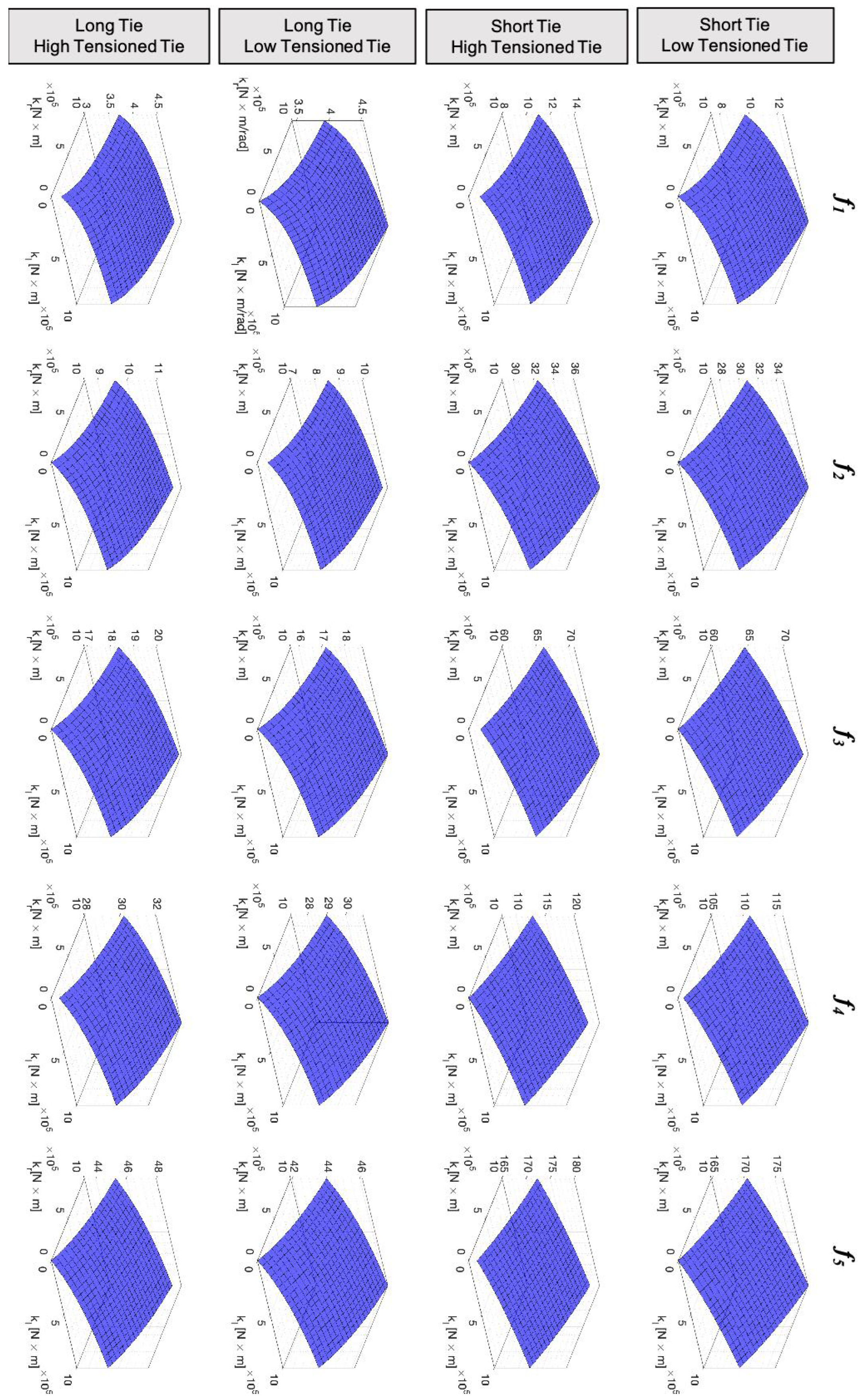
The GSA of the computational model output, , in Figure 1 is evaluated considering five output response Quantity of Interest (QoIs), i.e., , 1, …, 5, natural frequencies. A set of six statistically independent uncertain computational model input parameters (, 1, …, 6) are selected: Young modulus, E, mass density, , transversal square cross-section dimension, a, equivalent stiffness of left and right springs, and , and tensile axial force, N. For all the uncertain computational model input parameters, zero left truncated Gaussian distributions are selected, and their characteristics are summarized in Table 1. Different values of axial force, N, distribution mean values are used in order to account for the full range of possible axial loads in real ties in monumental buildings. In particular, two different cases are distinguished: low-tensioned and high-tensioned beams. Low-tensioned beams are characterized by axial load mean values equal to 0.1, 0.2, and 0.3× the axial load capacity of the tie, estimated assuming a material yield strength of = × , = 220 MPa. High-tensioned beams are characterized by axial load mean values equal to 0.4, 0.5, and 0.6× the axial load capacity of the tie. Elastic modulus, E, mass density, , and transversal square cross-section dimension, a, mean values are selected using common literature case studies [6,26,27]. The mean values of the spring stiffnesses, and , were determined through a preliminary parametric analysis, where the values of and were varied between the extreme conditions of pinned ( and equal to 0) and fixed ( and equal to Nm) boundary conditions. Subsequently, an average value of Nm was chosen, accompanied by a cov that adequately covers conditions near both pinned–pinned and fixed–fixed boundary conditions. Figure 2 illustrates the results obtained from this analysis. Since different results are expected in the case of short (i.e., length of tie rod lower than 5 m) and long (i.e., length of tie rod higher than 5 m) tie rods, two different tie rod lengths are considered: 5 m and 10 m. In all the considered cases, the most significant variation of the natural frequencies due to variations of the spring stiffnesses occur near the condition of pinned–pinned beams (i.e., and equal to zero), with an initial rapid increase of the natural frequencies beyond which an almost constant value is obtained, demonstrated by a progressive flattening of all the surfaces.
The first-order Sobol indices obtained for the considered cases of short low/high-tensioned tie rods and long low/high-tensioned tie rods are reported in Figure 3. Different results are obtained for each examined case. In particular, Young modulus, E, is the most influential parameters on the natural frequencies for low- and high-tensioned short tie rods; values of the first-order Sobol indices always higher than 40% are obtained for the natural frequencies 2 to 5 of the low-tensioned short tie rod and for the natural frequencies 3 to 5 of the high-tensioned short tie rod. Young modulus, E, has a significant influence on the higher-order natural frequencies of the low-tensioned and high-tensioned long tie rod with values of the first-order Sobol indices in between 20% and 40% for the higher-order natural frequencies and near zero values for the low-order natural frequencies. Mass density, , influences the first five natural frequencies of each considered case in a similar manner, with values of the first-order Sobol indices always in the range of 10–30%. The square cross-section transversal dimension, a, influences the first five natural frequencies in a different manner, being one of the most influential parameters in the case of high-tensioned short and long tie rods, with values of the first-order Sobol indices of around 20%. Axial force, N, is the most influential parameter on the natural frequencies of the long tie rod; values of the first-order Sobol indices always higher than 50% are obtained for the natural frequencies of the high-tensioned long tie rods, with the exception of the fifth natural frequency, and values of the first-order Sobol indices always higher than 40% are obtained for the low-order natural frequencies of low-tensioned long tie rods. Axial force, N, has a significant influence on the low-order natural frequencies of the low-tensioned and high-tensioned short tie rods with values of the first-order Sobol indices in between 20% and 60% for the low-order natural frequencies and near zero values for the higher-order natural frequencies. Finally, contrarily to what is expected, the stiffness of the left and right springs, and , have a negligible influence on the natural frequencies in all the considered cases, with values of the Sobol indices always near zero, with the exception of the first natural frequency of the low-tensioned short tie rod.
The GSA results highlight that the structural identification problem associated with ancient tie rods lacks a straightforward solution when considering natural frequencies as a target for the updating, in either deterministic and/or probabilistic settings. This means that the mathematical formulation of the inverse problem (i.e., choice of parameters to be estimated) needs to be set up in a different manner, depending on the length of the considered tie rod (short or long) and on the expected value of tensile axial force (low or high). This result is of utmost importance for practitioners involved in the examination of vulnerability, structural integrity, and seismic performance of historical masonry buildings equipped with ancient tie rods, providing practical recommendations to solve the issue.
In the following, the mathematical setting of the Bayesian inverse problem is properly set up, accounting for the GSA results.
The inverse problem for the probability estimates of the axial force, N, is well conditioned when the low-order natural frequencies are considered as reference (i.e., first three natural frequencies), especially in the case of short tie rods. When low-tensioned short tie rods are considered, the significant influence of the Young modulus, E, on the first five natural frequencies and the negligible influence of the axial force, N, on the higher-order natural frequencies can lead to misleading probability estimates of the axial force, N. Furthermore, the negligible influence of the spring stiffnesses, and , on the first five natural frequencies suggests that they should be considered as latent random variables, , in all the considered cases, with the exception of the low-tensioned short tie rods. The uncertainties about the Young modulus, E, the mass density, , and the square cross-section transversal dimension, a, may be estimated with a significant level of accuracy.
5. Bayesian Solution with Dynamic Data
According to the results of the GSA, Bayesian updating is carried out to solve the structural identification problem of the structural identification of ancient tie rods using natural frequencies as targets to distinguish the four cases: low-tensioned short and long tie rods and high-tensioned short and long tie rods. The reference dataset , used as the target for the updating procedure, is obtained from the numerical model using as actual true values of the input parameters those in Table 2, Table 3, Table 4 and Table 5 for each considered case. The measurements errors are applied by adding random errors into the simulated data. The errors are simulated based on [52] as
where indicates the natural frequencies obtained from the computational model using the initial parameter values (i.e., no noise natural frequencies), are random numbers sampled from a distribution with zero mean value and standard deviation equal to 1, and represents the level of noise in the dynamic measurements. In the following, of noise level is adopted. This choice reflects a typical range observed in experimental tests and is consistent with a previous study [52].
The length, l, of the tie beams is considered as a known measurable quantity since the effect of the anchorage length is considered in the different stiffnesses of the lateral springs. Posterior distributions are obtained using the MCMC–MH Algorithm 1. Convergency of MCMC was assessed by means of visual inspections of the trace plots showing the sampled values of parameters over iterations. Stationary chains displaying a random scatter around a central value without any apparent trend were ensured. Furthermore, autocorrelation plots were obtained between each sample and its lagged versions. A rapid decay of autocorrelations was obtained, suggesting good mixing and convergence. The Gelman–Rubin index was used, ensuring values close to 1, indicating convergence. Convergency was obtained after 400,000 runs of MCMC–MH for the low-tensioned short tie rods and after 450,000 runs of the MCMC–MH for all other cases.
It is worth remembering that most of the existing literature dynamic approaches for estimating the tensile axial force in ancient tie rods rely on a limited number of natural frequencies. In contrast, the proposed approach allows for the use of a greater number of natural frequencies as targets. This choice of natural frequencies as targets addresses the practical challenges associated with dynamic identification experimental tests on structural elements, particularly those situated at significant heights inside historic buildings where the installation of multiple accelerometers is often logistically challenging. This is the main reason for which mode shapes were not considered as targets, requiring the use of several accelerometers to be located along the tie rod axis. Furthermore, the association between natural frequencies and the vibration modes of tie rods is, in most cases, simple and straightforward, without the risk of mode switching. The primary objective of the proposed paper is to establish a robust mathematical framework capable of explicitly addressing modeling and measurement uncertainties, taking into account the outcomes of the global sensitivity analysis and the selection of natural frequencies as reference points. In the mathematical formulation discussed in Section 2, the mathematical framework can be easily adapted by appropriately selecting updating parameters and/or latent parameters and explicitly considering measurement errors.
5.1. Low-Tensioned Short Tie Rod
Following the mathematical formulation of the Bayesian updating framework in Section 2 and according to the results of the GSA in Section 4, for the low-tensioned short tie rod six updating parameters are considered (i.e., ): Young modulus, E, mass density, , cross-section transversal dimension, a, left and right spring stiffness, and , and axial tensile force, N. The effective length, l, of the tie is considered as a known measurable quantity. Zero left truncated Gaussian distributions are assumed as prior distributions of the uncertain parameters, whose mean and coefficient of variation, cov, are reported in Table 2.
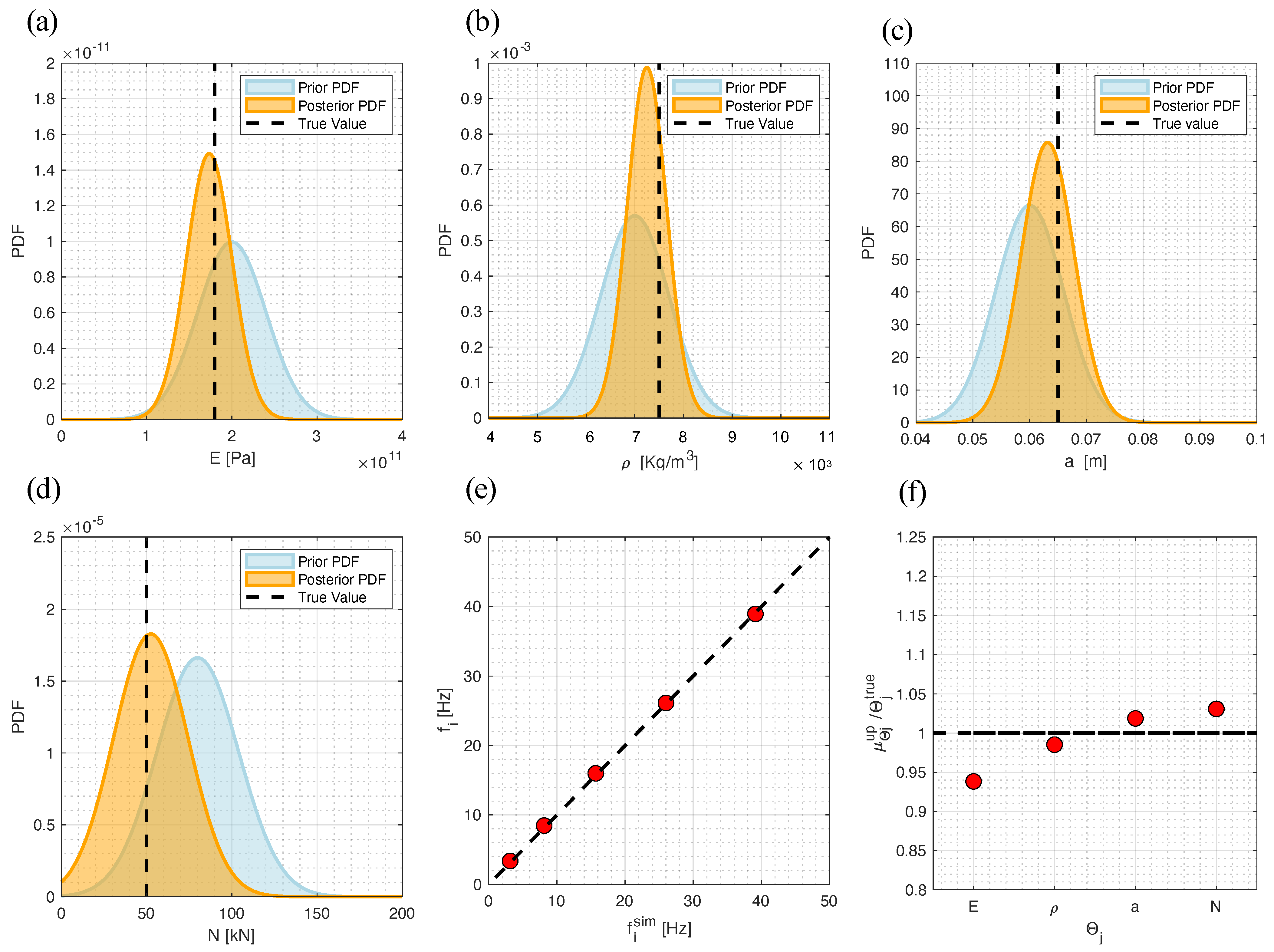
The results of the Bayesian updating framework (i.e., posterior distributions of the updating parameters, ) are reported in Figure 4. It is worth noting that the updating framework is able to modify the probability distributions of the updating parameters E, , and a, reducing the cov with respect to the prior distributions. The opposite behavior is obtained for the two spring stiffnesses, and , and the tensile axial force, N, with a cov of the posterior distributions greater than that of the prior distributions. These results were expected considering the results of GSA in Figure 3. When low-tensioned short tie rods are of interest, the most sensitive parameters on the QoIs are the Young modulus, E, the mass density, , and the transversal square cross-section dimension, a. The left and right spring stiffnesses, and , Sobol indices assume near zero values in all cases, with the exception of the first natural frequency, and the tensile axial force, N, Sobol indices assume values different from zero only when the first two natural frequencies are considered. However, it is worth observing that all the posterior distribution mean values, , move towards the true values (i.e., actual values used to simulate the reference dataset, D), showing the accuracy of the Bayesian updating framework to give useful information on the single-point solution of the structural identification problem. In order to further validate the proposed methodology, Figure 4g reports the comparison between the natural frequencies, , used as reference dataset and the natural frequencies, , obtained from the computational model driven by the posterior mean value of the updating parameters, . A good agreement between the reference natural frequencies and those predicted by the updated numerical model can be observed with a percentage relative difference (i.e., ) always lower than 1%. Furthermore, Figure 4h shows the ratio between the posterior mean value of the updated parameters, , and the true value, , of the computational model input parameters used to obtain the reference dataset, ; a ratio equal to 1 indicates a perfect match. Values of the posterior mean value, , of approximately 1.05 times the true value, , are obtained for the Young modulus, E, and the equivalent stiffness of the two lateral springs, and ; values of the posterior mean, , of approximately 0.95 times the true value, , are obtained for the mass density, , and the cross-section transversal dimension, a, value of posterior mean value, , of approximately 0.87 times the true value, , is obtained for the tensile axial force, N. The obtained results indicate that the computational model driven by the posterior mean value of the updating parameters, , provide a good representation of the structural system and that the tensile axial force value estimation is accurate. Furthermore, the obtained results show the capability of the Bayesian updating framework to be used for solving the structural identification problem of low-tensioned short tie rods being able to give useful information about the probability estimates of the most sensitive structural uncertain parameters (i.e., E, , and a).
5.2. High-Tensioned Short Tie Rod
Following the mathematical formulation of the Bayesian updating framework in Section 2 and according to the results of the GSA in Section 4, four updating parameters are considered (i.e., ) in the case of high-tensioned short tie rods: Young modulus, E, mass density, , cross-section transversal dimension, a, and axial tensile force, N; two latent random variables are considered, i.e., ): left and right spring stiffnesses, and . Zero left truncated Gaussian distributions are assumed as prior distributions of the updating parameters, whose mean and cov are reported in Table 3.
The results of the Bayesian updating framework (i.e., posterior distributions of the updating parameters, ) are reported in Figure 5. It is worth noting that the updating framework is able to modify the probability distributions of the updating parameters, , reducing the cov with respect to the cov of the prior distributions. Furthermore, the posterior distribution mean values, , of all the updating parameters move towards the true values (i.e., the actual values used to simulate the reference dataset, D). In particular, Figure 5f shows the ratio between the posterior mean value of the updated parameters, , and the true value, , of the computational model input parameters used to obtain the reference dataset, . Values of the ratio in between 0.94 and 1.03 are obtained for all the uncertain parameters, indicating an almost perfect match. It is worth noting that the estimation of the tensile axial force, N, posterior mean value, , is 1.03 times the true value. Finally, Figure 5e reports the comparison between the natural frequencies, , used as the reference dataset, , and the natural frequencies, , obtained from the computational model driven by the posterior mean value of the updating parameters, , and the mean value of the left and right spring stiffnesses; differences always lower than 2% are obtained. Differently from low-tensioned short tie rods, in this case Bayesian updating is able to provide accurate information on both the single-point value of the updating parameters and to reduce the uncertainty associated with the prior beliefs of all the uncertain parameters.
5.3. Low-Tensioned Long Tie Rod
Following the discussion in Section 2 and according to the results of the GSA in Section 4, the same mathematical setting of the Bayesian updating framework of the high-tensioned short tie rod is considered (i.e., , ). Zero left truncated Gaussian distributions are used as prior distributions, whose characteristics are reported in Table 4.
The results of the Bayesian updating framework (i.e., posterior distributions of the updating parameters, ) are reported in Figure 6. It is worth noting that the updating framework is able to modify the probability distributions of the updating parameters, reducing the cov with respect to the cov of the prior distributions, with the exception of the tensile axial force, N. Moreover, the posterior distributions mean values, , of all the updating parameters move towards the true values and the values of the ratio are between 0.95 and 1.05, indicating an almost perfect match between the two quantities (Figure 6f). Finally, also in this case, to further validate the proposed methodology the posterior mean value of the updating parameters, , is used as input for the computational model and the obtained natural frequencies, . The first five natural frequencies obtained by performing an eigenvalue analysis of this model are compared to the natural frequencies, , used as the target in the updating procedure. This comparison is shown in Figure 6e. An almost perfect match is observed, meaning that the updated computational model is reliable.
5.4. High-Tensioned Long Tie Rod
Bayesian updating is carried out to solve the structural identification problem of high-tensioned long tie rods using natural frequencies as a reference. Following the discussion in Section 2 and according to the results of the GSA in Section 4, the same mathematical setting of the Bayesian updating framework of the high-tensioned short tie rod and low-tensioned long tie rod is considered (i.e., , ). Zero left truncated Gaussian distributions are used as prior distributions; the values of prior mean and cov are reported in Table 5.
The results of the Bayesian updating framework (i.e., posterior distributions of the updating parameters, ) are reported in Figure 7. Also in this case, the proposed updating procedure is able to modify the probability distributions of the updating parameters, reducing the cov with respect to the cov of the prior distributions. Furthermore, the posterior distributions mean values, , of all the updating parameters move towards the true values and the ratio between the posterior mean value of the updated parameters, , and the true value, , of the computational model input parameters used to obtain the reference dataset, , are in between 1.00 and 1.05 for all the updating parameters, with the exception of the tensile axial force, N, for which the ratio assumes a value equal to 0.83 (Figure 7f). Figure 7e shows the comparison between the natural frequencies, and the natural frequencies , i = 1, …, 5 obtained from the computational model using the posterior mean value of the updated parameters, , showing a relative difference smaller than 0.8%.
Despite the existence of a difference between the true and the updated values of the tensile axial force, N, the good agreement between the true and the updated mean values of all the uncertain parameters, , and the good match between the natural frequencies used as the target for the updating and those obtained from the updated computational models show that the proposed Bayesian framework is robust and accurate in giving useful information on both single-point structural identification solutions and on probability estimates of the uncertain parameters.
6. Conclusions
In this paper, the Bayesian updating framework is mathematically formulated and used to solve the structural identification problem of ancient tie rods using natural frequencies as the target. Although this problem has received much attention in the literature, all the proposed approaches do not consider uncertainties and they are able to provide just a single-point solution using optimization functions that are often ill-posed, requiring regularization procedures. To bridge this gap, Bayesian updating is proposed as a robust methodology to obtain the solution of the structural identification problem of ancient tie rods using natural frequencies as a reference.
In particular, a global robust sensitivity analysis was carried out by means of Sobol variance decomposition and Sobol indices in order to properly select the updating parameters and to properly set up the mathematical formulation of the Bayesian framework. Since the sensitivity analysis indicated different behavior depending on beam length and axial force magnitude, two different beam lengths were considered (i.e., short and long ties) and two different levels of tension were selected (low- and high-tensioned ties). The global sensitivity analysis reveals that not all computational model input parameters have the same influence on natural frequencies. Additionally, the stiffness of lateral rotational springs has a negligible impact on natural frequencies, except in cases of low-tensioned short tie rods. This finding underscores the need for a distinct formulation of the inverse problem, determining which parameters to estimate, depending on the tie rod’s length (short or long) and the expected tensile axial force (low or high). The obtained results are of utmost importance for practitioners interested in assessing the vulnerability, structural integrity, and seismic performance of historical masonry buildings equipped with ancient tie rods, offering practical recommendations for problem set up and resolution.
Second, five natural frequencies were used as targets in the updating framework for each considered case. The obtained results demonstrated the effectiveness of the proposed approach in accurately estimate the single-point solutions of the structural identification problem, obtaining a reliable updated computational model. Furthermore, the proposed procedure has been shown to be effective in providing probability estimates of the modeling uncertainty involved in the problem. In particular, regarding the estimation of axial load—crucial for assessing the integrity of both the rod and the entire structure it supports—it is essential to note that the Bayesian approach enables the estimation of probability distributions by incorporating data while accounting for measurement and model uncertainties through the definition of appropriate probabilistic models. This allows the reliable determination of the probability distribution of axial load by integrating information coming from experimental data and computational model parameters. Additionally, it is noteworthy that, in each scenario considered, it is feasible to obtain an estimate of the mean value of the posterior distribution of axial load, which varies by a maximum of 0.15% (i.e., low-tensioned tie rods) and a minimum of 0.03% (high-tensioned short tie rods).
Works are in progress in order to assess the effectiveness of the proposed procedure to solve the structural identification problem of ancient tie rods using experimental noisy modal data exploring different types of sampling methods to evaluate the posterior distributions of all the uncertain parameters.
Author Contributions
Conceptualization, C.P. and M.G.; data curation, C.P.; formal analysis, C.P.; funding acquisition, M.G.; investigation, C.P.; methodology, C.P.; project administration, M.G.; resources, M.G.; software, C.P. and M.G.; supervision, M.G.; validation, C.P. and M.G.; visualization, C.P.; writing—original draft preparation, C.P.; writing—review and editing, M.G. All authors have read and agreed to the published version of the manuscript.
Funding
This work has been funded by the European Union—NextGenerationEU under the Italian Ministry of University and Research (MUR) National Innovation Ecosystem grant ECS00000041- VITALITY-CUP J97G22000170005.
Institutional Review Board Statement
Not applicable.
Informed Consent Statement
Not applicable.
Data Availability Statement
The raw data supporting the conclusions of this article will be made available by the authors on request.
Conflicts of Interest
The authors declare no conflicts of interest.
References
- Amabili, M.; Carra, S.; Collini, L.; Garziera, R.; Panno, A. Estimation of tensile force in tie-rods using a frequency-based identification method. J. Sound Vib. 2010, 329, 2057–2067. [Google Scholar] [CrossRef]
- Calderini, C.; Lagomarsino, S. Seismic Response of Masonry Arches Reinforced by Tie-Rods: Static Tests on a Scale Model. J. Struct. Eng. 2015, 141, 04014137. [Google Scholar] [CrossRef]
- Milani, G.; Shehu, R.; Valente, M. A kinematic limit analysis approach for seismic retrofitting of masonry towers through steel tie-rods. Eng. Struct. 2018, 160, 212–228. [Google Scholar] [CrossRef]
- Podesta, S.; Scandolo, L. Earthquakes and tie-rods: Assessment, design, and ductility issues. Int. J. Archit. Herit. 2019, 13, 329–339. [Google Scholar] [CrossRef]
- Calderini, C.; Piccardo, P.; Vecchiattini, R. Experimental characterization of ancient metal tie-rods in historic masonry buildings. Int. J. Archit. Herit. 2019, 13, 425–437. [Google Scholar] [CrossRef]
- De Falco, A.; Resta, C.; Sevieri, G. Sensitivity analysis of frequency-based tie-rod axial load evaluation methods. Eng. Struct. 2021, 229, 111568. [Google Scholar] [CrossRef]
- Coïsson, E.; Collini, L.; Ferrari, L.; Garziera, R.; Riabova, K. Dynamical assessment of the work conditions of reinforcement tie-rods in historical masonry structures. Int. J. Archit. Herit. 2019, 13, 358–370. [Google Scholar] [CrossRef]
- Cescatti, E.; Da Porto, F.; Modena, C. Axial force estimation in historical metal tie-rods: Methods, influencing parameters, and laboratory tests. Int. J. Archit. Herit. 2019, 13, 317–328. [Google Scholar] [CrossRef]
- Luca, F.; Manzoni, S.; Cigada, A.; Frate, L. A vibration-based approach for health monitoring of tie-rods under uncertain environmental conditions. Mech. Syst. Signal Process. 2022, 167, 108547. [Google Scholar] [CrossRef]
- Bati, S.B.; Tonietti, U. Experimental methods for estimating in situ tensile force in tie-rods. J. Eng. Mech. 2001, 127, 1275–1283. [Google Scholar] [CrossRef]
- Tullini, N. Bending tests to estimate the axial force in slender beams with unknown boundary conditions. Mech. Res. Commun. 2013, 53, 15–23. [Google Scholar] [CrossRef]
- Sorace, S. Parameter models for estimating in-situ tensile force in tie-rods. J. Eng. Mech. 1996, 122, 818–825. [Google Scholar] [CrossRef]
- Collini, L.; Garziera, R.; Riabova, K. Vibration analysis for monitoring of ancient tie-rods. Shock Vib. 2017, 2017, 7591749. [Google Scholar] [CrossRef]
- Gioffré, M.; Cavalagli, N.; Pepi, C.; Trequattrini, M. Laser doppler and radar interferometer for contactless measurements on unaccessible tie-rods on monumental buildings: Santa Maria della Consolazione Temple in Todi. J. Phys. Conf. Ser. 2017, 778, 012008. [Google Scholar] [CrossRef]
- Gentile, C.; Poggi, C.; Ruccolo, A.; Vasic, M. Vibration-based assessment of the tensile force in the tie-rods of the Milan Cathedral. Int. J. Archit. Herit. 2019, 13, 411–424. [Google Scholar] [CrossRef]
- Resta, C.; Chellini, G.; De Falco, A. Dynamic assessment of axial load in tie-rods by means of acoustic measurements. Buildings 2020, 10, 23. [Google Scholar] [CrossRef]
- Tullini, N.; Laudiero, F. Dynamic identification of beam axial loads using one flexural mode shape. J. Sound Vib. 2008, 318, 131–147. [Google Scholar] [CrossRef]
- Rebecchi, G.; Tullini, N.; Laudiero, F. Estimate of the axial force in slender beams with unknown boundary conditions using one flexural mode shape. J. Sound Vib. 2013, 332, 4122–4135. [Google Scholar] [CrossRef]
- Li, S.; Reynders, E.; Maes, K.; De Roeck, G. Vibration-based estimation of axial force for a beam member with uncertain boundary conditions. J. Sound Vib. 2013, 332, 795–806. [Google Scholar] [CrossRef]
- Camassa, D.; Castellano, A.; Fraddosio, A.; Miglionico, G.; Piccioni, M.D. Dynamic identification of tensile force in tie-rods by interferometric radar measurements. Appl. Sci. 2021, 11, 3687. [Google Scholar] [CrossRef]
- Campagnari, S.; Di Matteo, F.; Manzoni, S.; Scaccabarozzi, M.; Vanali, M. Estimation of axial load in tie-rods using experimental and operational modal analysis. J. Vib. Acoust. 2017, 139. [Google Scholar] [CrossRef]
- Duvnjak, I.; Ereiz, S.; Damjanović, D.; Bartolac, M. Determination of axial force in tie rods of historical buildings using the model-updating technique. Appl. Sci. 2020, 10, 6036. [Google Scholar] [CrossRef]
- Gentilini, C.; Marzani, A.; Mazzotti, M. Nondestructive characterization of tie-rods by means of dynamic testing, added masses and genetic algorithms. J. Sound Vib. 2013, 332, 76–101. [Google Scholar] [CrossRef]
- Battini, C.; Calderini, C.; Vecchiattini, R. 3D Digital Survey of Iron Tie-Rods in Masonry Buildings: Cross-Sections Analysis and Error Estimation. Int. J. Archit. Herit. 2019, 13, 438–450. [Google Scholar] [CrossRef]
- Calderini, C.; Vecchiattini, R.; Battini, C.; Piccardo, P. Mechanical and Metallographic Characterization of Iron Tie-Rods in Masonry Buildings: An Experimental Study. In Structural Analysis of Historical Constructions: Anamnesis, Diagnosis, Therapy, Controls; CRC Press: Boca Raton, FL, USA, 2016; pp. 1293–1300. [Google Scholar]
- Makoond, N.; Pelà, L.; Molins, C. Robust estimation of axial loads sustained by tie-rods in historical structures using Artificial Neural Networks. Struct. Health Monit. 2022, 22, 14759217221123326. [Google Scholar] [CrossRef]
- Pepi, C.; Grigoriu, M.D.; Gioffrè, M. Identification of Tie-Rod Properties in Monumental Buildings under Uncertainty. In Materials Research Proceedings; Association of American Publishers: Washington, DC, USA, 2023; Volume 26, pp. 567–572. [Google Scholar]
- Joyce, J. Bayes’ theorem. 2003. [Google Scholar]
- Beck, J.L.; Katafygiotis, L.S. Updating models and their uncertainties. I: Bayesian statistical framework. J. Eng. Mech. 1998, 124, 455–461. [Google Scholar] [CrossRef]
- Vanik, M.W.; Beck, J.L.; Au, S.K. Bayesian probabilistic approach to structural health monitoring. J. Eng. Mech. 2000, 126, 738–745. [Google Scholar] [CrossRef]
- Simoen, E.; Papadimitriou, C.; Lombaert, G. On prediction error correlation in Bayesian model updating. J. Sound Vib. 2013, 332, 4136–4152. [Google Scholar] [CrossRef]
- Pepi, C.; Gioffre, M.; Grigoriu, M. Bayesian inference for parameters estimation using experimental data. Probab. Eng. Mech. 2020, 60, 103025. [Google Scholar] [CrossRef]
- Pepi, C.; Gioffre’, M.; Grigoriu, M.D. Parameters identification of cable stayed footbridges using Bayesian inference. Meccanica 2019, 54, 1403–1419. [Google Scholar] [CrossRef]
- García-Macías, E.; Ierimonti, L.; Venanzi, I.; Ubertini, F. An innovative methodology for online surrogate-based model updating of historic buildings using monitoring data. Int. J. Archit. Herit. 2021, 15, 92–112. [Google Scholar] [CrossRef]
- Valikhani, M.; Jahangiri, V.; Ebrahimian, H.; Moaveni, B.; Liberatore, S.; Hines, E. Inverse modeling of wind turbine drivetrain from numerical data using Bayesian inference. Renew. Sustain. Energy Rev. 2023, 171, 113007. [Google Scholar] [CrossRef]
- Kurent, B.; Friedman, N.; Ao, W.K.; Brank, B. Bayesian updating of tall timber building model using modal data. Eng. Struct. 2022, 266, 114570. [Google Scholar] [CrossRef]
- Sevieri, G.; De Falco, A. Dynamic structural health monitoring for concrete gravity dams based on the Bayesian inference. J. Civ. Struct. Health Monit. 2020, 10, 235–250. [Google Scholar] [CrossRef]
- Monchetti, S.; Viscardi, C.; Betti, M.; Clementi, F. Comparison between Bayesian updating and approximate Bayesian computation for model identification of masonry towers through dynamic data. Bull. Earthq. Eng. 2023, 1–19. [Google Scholar] [CrossRef]
- Peng, Z.; Wang, Z.; Yin, H.; Bai, Y.; Dong, K. A new Bayesian finite element model updating method based on information fusion of multi-source Markov chains. J. Sound Vib. 2022, 526, 116811. [Google Scholar] [CrossRef]
- Box, G.E.; Tiao, G.C. Bayesian Inference in Statistical Analysis; John Wiley & Sons: Hoboken, NJ, USA, 2011. [Google Scholar]
- Gardoni, P.; Der Kiureghian, A.; Mosalam, K.M. Probabilistic capacity models and fragility estimates for reinforced concrete columns based on experimental observations. J. Eng. Mech. 2002, 128, 1024–1038. [Google Scholar] [CrossRef]
- Sevieri, G.; De Falco, A.; Andreini, M.; Matthies, H.G. Hierarchical Bayesian framework for uncertainty reduction in the seismic fragility analysis of concrete gravity dams. Eng. Struct. 2021, 246, 113001. [Google Scholar] [CrossRef]
- Hastings, W.K. Monte Carlo sampling methods using Markov chains and their applications. Biometrika 1970, 57, 97–109. [Google Scholar] [CrossRef]
- Berg, B.A. Markov Chain Monte Carlo Simulations and Their Statistical Analysis: With Web-Based Fortran Code; World Scientific Publishing Company: Singapore, 2004. [Google Scholar]
- Geyer, C.J. Introduction to Markov Chain Monte Carlo. In Handbook of Markov Chain Monte Carlo; Taylor & Francis: Oxfordshire, UK, 2011; p. 45. [Google Scholar]
- Konakli, K.; Sudret, B. Global sensitivity analysis using low-rank tensor approximations. Reliab. Eng. Syst. Saf. 2016, 156, 64–83. [Google Scholar] [CrossRef]
- Tosin, M.; Côrtes, A.M.; Cunha, A. A Tutorial on Sobol’Global Sensitivity Analysis Applied to Biological Models. In Networks in Systems Biology: Applications for Disease Modeling; Springer: Cham, Switzerland, 2020; pp. 93–118. [Google Scholar]
- Sudret, B. Global sensitivity analysis using polynomial chaos expansions. Reliab. Eng. Syst. Saf. 2008, 93, 964–979. [Google Scholar] [CrossRef]
- Ghanem, R.; Higdon, D.; Owhadi, H. Handbook of Uncertainty Quantification; Springer: New York, NY, USA, 2017. [Google Scholar]
- Saltelli, A. Sensitivity analysis for importance assessment. Risk Anal. 2002, 22, 579–590. [Google Scholar] [CrossRef] [PubMed]
- Zhang, X.Y.; Trame, M.N.; Lesko, L.J.; Schmidt, S. Sobol sensitivity analysis: A tool to guide the development and evaluation of systems pharmacology models. CPT Pharmacometr. Syst. Pharmacol. 2015, 4, 69–79. [Google Scholar] [CrossRef] [PubMed]
- Liu, K.; Yan, R.J.; Soares, C.G. Damage identification in offshore jacket structures based on modal flexibility. Ocean Eng. 2018, 170, 171–185. [Google Scholar] [CrossRef]
Figure 1.
Scheme for axially loaded beam-like structure.

Figure 2.
Response surfaces of the first five natural frequencies varying the restraint spring stiffnesses, and .
Figure 2.
Response surfaces of the first five natural frequencies varying the restraint spring stiffnesses, and .

Figure 3.
Sensitivity analysis results (i.e., Sobol indices) for the different considered cases.

Figure 4.
Posterior PDF of the updated parameters: (a) Young modulus, E, (b) mass density, , (c) cross section transversal dimension, a, (d) stiffness of left spring, , (e) stiffness of right spring, , and (f) axial load, N. Results comparison: (g) natural frequencies , i = 1, …, 5 obtained from the computational model using the posterior mean value of the updated parameters, , and natural frequencies used as reference; (h) posterior mean value of the updated parameters, , and true value, .

Figure 5.
Posterior PDF of the updated parameters: (a) Young modulus, E, (b) mass density, , (c) cross section transversal dimension, a, (d) axial load, N. Results comparison: (e) natural frequencies , i = 1, …, 5 obtained from the computational model using the posterior mean value of the updated parameters, , and natural frequencies used as reference; (f) posterior mean value of the updated parameters, , and true value, .

Figure 6.
Posterior PDF of the updated parameters: (a) Young modulus, E, (b) mass density, , (c) cross section transversal dimension, a, (d) axial load, N. Results comparison: (e) natural frequencies , i = 1, …, 5 obtained from the computational model using the posterior mean value of the updated parameters, , and natural frequencies used as reference; (f) posterior mean value of the updated parameters, , and true value, .

Figure 7.
Posterior PDF of the updated parameters: (a) Young modulus, E, (b) mass density, , (c) cross section transversal dimension, a, (d) axial load, N. Results comparison: (e) natural frequencies , i = 1, …, 5 obtained from the computational model using the posterior mean value of the updated parameters, , and natural frequencies used as reference; (f) posterior mean value of the updated parameters, , and true value, .


Table 1.
Uncertain computational model input parameters and probability distributions for sensitivity analysis.
Table 1.
Uncertain computational model input parameters and probability distributions for sensitivity analysis.
| Parameter | Mean | Cov | Distribution |
|---|---|---|---|
| E | 2.0 × [Pa] | 0.25 | Truncated Gaussian |
| 7500 [Kg/] | 0.10 | Truncated Gaussian | |
| a | 0.07 [m] | 0.10 | Truncated Gaussian |
| 400,000 [N × m] | 0.30 | Truncated Gaussian | |
| 400,000 [N × m] | 0.30 | Truncated Gaussian | |
| N-low-tensioned cases | 0.1× [N] | 0.30 | Truncated Gaussian |
| 0.2× [N] | 0.30 | Truncated Gaussian | |
| 0.3× [N] | 0.30 | Truncated Gaussian | |
| N-high-tensioned cases | 0.4× [N] | 0.30 | Truncated Gaussian |
| 0.5× [N] | 0.30 | Truncated Gaussian | |
| 0.6× [N] | 0.30 | Truncated Gaussian |
Table 2.
Comparison of actual and predicted parameters obtained for low-tensioned short tie rod.
| Prior Distribution | Posterior Distribution | ||||
|---|---|---|---|---|---|
| True Value | Mean Value | Cov | Mean Value | Cov | |
| E [Pa] | 1.80 × | 2.00 × | 0.30 | 1.867 × | 0.12 |
| [Kg/] | 7500 | 7000 | 0.10 | 7232 | 0.06 |
| a [m] | 0.065 | 0.06 | 0.10 | 0.062 | 0.06 |
| [N × m] | 200,000 | 300,000 | 0.30 | 240,890 | 0.35 |
| [N × m] | 200,000 | 300,000 | 0.30 | 212,480 | 0.46 |
| N [N] | 50,000 | 80,000 | 0.30 | 43,699 | 0.48 |
Table 3.
Comparison of actual and predicted parameters obtained for high-tensioned short tie rod.
| Prior Distribution | Posterior Distribution | ||||
|---|---|---|---|---|---|
| True Value | Mean Value | Cov | Mean Value | Cov | |
| E [Pa] | 1.80 × | 2.00 × | 0.30 | 1.689 × | 0.14 |
| [Kg/] | 7500 | 7000 | 0.10 | 7389 | 0.07 |
| a [m] | 0.065 | 0.06 | 0.10 | 0.066 | 0.06 |
| [N × m] | 200,000 | 300,000 | 0.30 | - | - |
| [N × m] | 200,000 | 300,000 | 0.30 | - | - |
| N [N] | 400,000 | 500,000 | 0.30 | 412,360 | 0.19 |
Table 4.
Comparison of actual and predicted parameters obtained for low-tensioned long tie rod.
| Prior Distribution | Posterior Distribution | ||||
|---|---|---|---|---|---|
| True Value | Mean Value | Cov | Mean Value | Cov | |
| E [Pa] | 1.80 × | 2.00 × | 0.30 | 1.735 × | 0.15 |
| [Kg/] | 7500 | 7000 | 0.10 | 7255 | 0.09 |
| a [m] | 0.065 | 0.06 | 0.10 | 0.063 | 0.06 |
| [N × m] | 200,000 | 300,000 | 0.30 | - | - |
| [N × m] | 200,000 | 300,000 | 0.30 | - | - |
| N [N] | 50,000 | 80,000 | 0.30 | 52,408 | 0.41 |
Table 5.
Comparison of actual and predicted parameters obtained for high-tensioned long tie rod.
| Prior Distribution | Posterior Distribution | ||||
|---|---|---|---|---|---|
| True Value | Mean Value | Cov | Mean Value | Cov | |
| E [Pa] | 1.80 × | 2.00 × | 0.30 | 1.824 × | 0.13 |
| [Kg/] | 7500 | 7000 | 0.10 | 7799 | 0.07 |
| a [m] | 0.065 | 0.06 | 0.10 | 0.066 | 0.06 |
| [N × m] | 200,000 | 300,000 | 0.30 | - | - |
| [N × m] | 200,000 | 300,000 | 0.30 | - | - |
| N [N] | 400,000 | 500,000 | 0.30 | 419,750 | 0.16 |
Disclaimer/Publisher’s Note: The statements, opinions and data contained in all publications are solely those of the individual author(s) and contributor(s) and not of MDPI and/or the editor(s). MDPI and/or the editor(s) disclaim responsibility for any injury to people or property resulting from any ideas, methods, instructions or products referred to in the content. |
© 2024 by the authors. Licensee MDPI, Basel, Switzerland. This article is an open access article distributed under the terms and conditions of the Creative Commons Attribution (CC BY) license (https://creativecommons.org/licenses/by/4.0/).
Share and Cite
MDPI and ACS Style
Pepi, C.; Gioffrè, M. Bayesian Updating for Random Tensile Force Identification of Ancient Tie Rods Using Modal Data. Appl. Sci. 2024, 14, 3698. https://0-doi-org.brum.beds.ac.uk/10.3390/app14093698
AMA Style
Pepi C, Gioffrè M. Bayesian Updating for Random Tensile Force Identification of Ancient Tie Rods Using Modal Data. Applied Sciences. 2024; 14(9):3698. https://0-doi-org.brum.beds.ac.uk/10.3390/app14093698
Chicago/Turabian StylePepi, Chiara, and Massimiliano Gioffrè. 2024. "Bayesian Updating for Random Tensile Force Identification of Ancient Tie Rods Using Modal Data" Applied Sciences 14, no. 9: 3698. https://0-doi-org.brum.beds.ac.uk/10.3390/app14093698
Note that from the first issue of 2016, this journal uses article numbers instead of page numbers. See further details here.