

A Critical Review of the Modelling Tools for the Reactive Transport of Organic Contaminants

Institute for Ecology of Industrial Areas, 6 Kossutha St., 40-844 Katowice, Poland
*
Author to whom correspondence should be addressed.
Appl. Sci. 2024, 14(9), 3675; https://0-doi-org.brum.beds.ac.uk/10.3390/app14093675
Submission received: 29 February 2024
/
Revised: 17 April 2024
/
Accepted: 23 April 2024
/
Published: 25 April 2024
(This article belongs to the Special Issue Environmental Bioaccumulation and Assessment of Toxic Elements)
Abstract
:Featured Application
This paper helps to summarize the most relevant information on reactive transport models used to simulate the transport of hydrocarbons. The authors hope that this paper will be very useful for future modelers, stakeholders, and scientists, and will help them to select the most appropriate tools or to create new models.
Abstract
The pollution of groundwater and soil by hydrocarbons is a significant and growing global problem. Efforts to mitigate and minimise pollution risks are often based on modelling. Modelling-based solutions for prediction and control play a critical role in preserving dwindling water resources and facilitating remediation. The objectives of this article are to: (i) to provide a concise overview of the mechanisms that influence the migration of hydrocarbons in groundwater and to improve the understanding of the processes that affect contamination levels, (ii) to compile the most commonly used models to simulate the migration and fate of hydrocarbons in the subsurface; and (iii) to evaluate these solutions in terms of their functionality, limitations, and requirements. The aim of this article is to enable potential users to make an informed decision regarding the modelling approaches (deterministic, stochastic, and hybrid) and to match their expectations with the characteristics of the models. The review of 11 1D screening models, 18 deterministic models, 7 stochastic tools, and machine learning experiments aimed at modelling hydrocarbon migration in the subsurface should provide a solid basis for understanding the capabilities of each method and their potential applications.
1. Introduction
Contamination of soil and groundwater by organic pollutants is a global problem that needs to be addressed, especially at historically contaminated industrial areas, such as brownfields or abandoned sites. Despite their tainted past, these areas, often located in urban industrial regions and low-income communities, hold potential for revitalization through remediation efforts. In 2016, 1.38 million potentially contaminated sites were registered, 98% of them in 11 countries [1]. According to projections, this number is likely to increase, as potentially polluting activities took place at a total of 2.8 million sites [2,3,4]. Mineral oils and heavy metals are the main contaminants, accounting for about 60% of soil pollution.
In the EEA countries, around 235,000 contaminated sites have been remediated [4], which corresponds to 17% of the potentially contaminated sites currently registered. The cost of managing contaminated soils in Europe amounts to around 6.5 billion euros per year [5]. The cost of a site investigation is usually between EUR 5000 and EUR 50,000 (60% of reported cases), while the cost of remediation projects is usually between EUR 50,000 and EUR 500,000 (40% of reported cases) [3]. The cost of remediation and restoration can be even higher, ranging from EUR 150,000 to EUR 2 billion, as it is difficult to separate these measures [6]. As hydrocarbon pollution is a widespread problem, many spatial planners and decision-makers are faced with the problem of rapid and cost-effective remediation. Decisions on remediation strategies require tools and guidelines that provide a reliable estimate of the time and labour required to reduce the plume and source of contamination [7,8]. Numerical modelling can be an important method to study the fate of hydrocarbons in the aquatic environment [9,10,11]. It can precede any on-site action, estimate the extent of contamination, and help select the most effective and economical remediation methods. They can therefore help scientists, engineers, and decision makers to significantly improve their knowledge and optimize site management. Numerical models can also help to reduce the costs associated with long-term monitoring programs and sampling campaigns by identifying biogeochemical processes and quantifying their long-term effects.
One of the first applications of computer modelling to estimate groundwater flow dates back to the 1960s when Remson, together with Appel and Webster, proposed the use of finite differences and digital computers to track water flow [12], but very few involved hydrocarbon seeps. Since the 1970s, however, the number of journal articles describing models for the transport of hydrocarbons in water has increased (Figure 1), with an abrupt increase in recent years. There have been several breakthroughs in knowledge during these decades, e.g., the involvement of microorganisms in oil spills was described in detail as early as the 1970s [13], and in the same year a fundamental theoretical concept of the chemical and biological processes associated with the presence of hydrocarbons in soil and groundwater was formulated [14]. The theoretical and numerical definition and realisation of multiphase transport of hydrocarbons can also be regarded as a fundamental advance in knowledge in the 1980s [15,16].
The first numerical models were based on a single organic pollutant whose degradation was simulated either by a single electron acceptor [17,18] or by several electron acceptors [19]. In the 1990s, the groundwater flow model—MODFLOW—was coupled with the reaction modules, and since then the term multispecies reactive transport has become established [20,21]. An important part of the hydrocarbon studies has also been the development of standards for soil and water remediation based on the models and their uncertainty and sensitivity analyses [22,23,24,25], timeframes for remediation [26,27,28], and health risk assessments related to indoor and outdoor exposure [29,30,31]. These parameters are of critical importance to practitioners and environmental engineers whose goal is to revitalise polluted sites or return them to their natural state. The main turning points in hydrocarbon research have been the introduction of new remediation methods such as the use of nanoparticles [32,33], new devices/methods to measure pollutant concentrations [34,35,36], detailed monitoring [37,38,39,40,41], or the coupling of other techniques such as isotope measurements [42,43,44].
Remediation of hydrocarbon contaminated sites is an emerging field of research [45]. It has been reported that the number of papers published annually on this topic is increasing at an average annual growth rate of 9.22% [46]. Despite this large number of publications, only a few of them mention the need for further progress, which still needs to be improved, as hydrocarbons are among the most hazardous pollutants, posing a high risk to health and the aquatic environment.
So what does the future of hydrocarbon research look like? Looking at the articles from the last decades, one might conclude that some studies will continue to be site-specific, focusing on high-risk sites [47,48], large-scale sites [48,49,50,51,52], or areas with extreme conditions [53,54,55,56,57]. Certainly, some articles will refer to laboratory experiments and the dynamics of reactions affecting the attenuation of hydrocarbons in soils and water [58,59,60]. When it comes to studying the fate of hydrocarbons in the subsurface, there is still room for mesoscale laboratory studies [61,62,63] or field experiments [64,65,66,67], as these types of studies better reflect the ongoing processes in heterogeneous soils and the growth of bacterial communities in the quasi-real environment. It is likely that new studies will be required to address the remaining unresolved challenges in remediating hydrocarbon-contaminated soils, such as heterogeneity [68,69], realistic representation of volatile compound transport [70,71], accurate injection of oxidants or reductants [72,73], and modelling of these processes with new modelling tools [74,75] or with models that are well known but applied in novel ways [76,77]. Overviews of the fate and transport of organic pollutants and their bioremediation with updated knowledge of the mechanisms, the dynamics of the processes, and new modelling tools will also play an important role for future researchers to keep up with the trends [45,78,79,80].
Stochastic models are particularly interesting and can be used to construct probable scenarios, policy rules, guidelines, and risk assessments. They seem to be good solutions for complex systems where heterogeneity and randomness play a crucial role in the distribution of pollutants. These tools are described in the following sections together with examples of their application. A brief description of the application of machine learning methods in hydrogeological modelling is also included. This method, which offers high accuracy, is dynamically integrated into hydrological and hydrogeological modelling [56,81,82].
The aim of this article is to provide a comprehensive overview of existing solutions for modelling the transport and removal of hydrocarbons from the subsurface. This is facilitated by several objectives: the description of the processes controlling hydrocarbon migration and remediation required to build the conceptual model, the presentation of the most common mathematical models with their characteristics and limitations, and the presentation of the theoretical background of the different modelling approaches and their weaknesses and strengths.
This article is aimed at several groups: practitioners and experts in the field who opt for simpler solutions that are intuitive, have a user interface, and allow for a rich visualisation that can be presented to stakeholders and decision makers. For this reason, the deterministic 1D and 3D models are described in detail. In addition, this paper may be useful for scientists and developers who need a strong theoretical background and are interested in more sophisticated tools based on probability theory and machine learning algorithms. The paper could also be useful for future users and modelers. Therefore, the audience that can gain insights from reading this paper is broad, and the paper should help in selecting the optimal modelling tool or combination of different models when assessing contaminated sites.
To summarize, this paper provides a roadmap for navigating between different approaches and models for predicting the fate of hydrocarbons in the subsurface. In addition to a brief overview of the history of discoveries in the field of hydrocarbon migration and removal from soils and groundwater, the paper provides insights into current and future trends in modelling and research. The novelty of this paper lies in the wealth of information to help future users make informed decisions and in the comparison of different approaches, including the application of machine learning algorithms to reactive transport. In addition, to the best of the authors’ knowledge, it provides the most detailed description of stochastic models used to reproduce hydrocarbon migration in the subsurface.
2. Processes
As early as the 1970s, the fate of oil spills was described in terms of various processes, including advection, spreading and dispersion, dissolution, biodegradation, evaporation, and emulsification. However, due to the limited or lack of knowledge of analytical expressions for many of these processes and associated factors, the mathematical models were often simplified, resulting in several important processes being omitted [83]. In the early 1980s, the understanding of the fate and behaviour of spilled crude oil was extended to nine processes: advection, dispersion, evaporation, dissolution, emulsification, auto-oxidation, biodegradation, and sinking/sedimentation [84]. In the mathematical models, however, the focus remained on advection, dispersion, and evaporation.
However, stochastic reactive 3D flow transport was developed as early as 1985, taking into account first-order kinetics for degradation, adsorption, dispersion, spreading and retardation through a doubly porous medium [85]. This method proved to be sophisticated, cost-effective, and robust and enabled accurate calculations of pollutant concentrations in the plume of chlorinated hydrocarbons. Almost simultaneously, the BIOPLUME model [17,86] was developed, an early attempt to link 2D transport of dissolved hydrocarbons and biodegradation under low-oxygen conditions. This model was applied in aerobic aquifers to predict the release of organic pollutants by various processes such as convection, dispersion, mixing, and biodegradation.
In the 1980s, when computing power was still relatively modest, two parallel branches of modelling (deterministic and stochastic) were successfully formulated and implemented (Figure 2). At that time, however, modelling was primarily the preserve of engineers, scientists, and professionals who had the necessary knowledge and tools. After almost a decade, in response to the needs of practitioners, screening tools were developed to facilitate the use of these models in a user-friendly spreadsheet environment [87,88,89]. Another significant advance was the introduction of the modular open-source 3D groundwater flow model MODFLOW, together with MT3D and RT3D, which enabled the simulation of the transport of multiple species in water.
In the following sections, the processes controlling the migration of hydrocarbons are described in detail to improve the understanding of the underlying theory behind the algorithms incorporated into the mathematical models. While most models had to account for transport in the saturated zone, a few also can consider infiltration through the vadose zone. In addition, key processes such as dispersion, sorption, and biodegradation, which play a central role in controlling the concentrations of solutes in the subsurface, are explained in detail. Furthermore, lesser-known processes pertaining to the removal of contaminants, such as biodegradation or chemical oxidation, which are modelled by the included tools, are also discussed. Some additional processes that are not explicitly considered in the models but are important for the natural attenuation, leakage, and transport of hydrocarbons can be found in the cited literature [46,90,91,92,93].
Figure 2.
Timeline of key knowledge breakthroughs and models for the transport of hydrocarbon, references: [12,83,84,94,95,96,97,98].

2.1. Transport
Despite numerous studies and years of research into hydrocarbon migration, the process remains in the discovery phase. When hydrocarbons enter an aquifer, they move downward under gravity through a vadose zone and partition into subsequent phases [99,100,101,102]:
- mobile fluid—the mobile free product, mobile non-aqueous liquid phase (NAPL);
- residual liquid—an immobile, trapped portion of the hydrocarbons that occurs above and/or below the water table and is an additional, persistent source of contamination;
- aqueous—dissolved in groundwater and soil moisture;
- sorbed—adsorbed to soil particles;
- volatile—hydrocarbons in the gaseous state, which have evaporated (depending on Henry’s constant) from the free product layer and/or dissolved phase and occur mainly in the unsaturated zone.
Once NAPLs reach the water table, they can form a visible free-product layer that floats on the surface of the groundwater—LNAPLs (Figure 3). The soluble compounds are dissolved while they are denser than water. DNAPLs migrate vertically downwards into the saturated zone.
Both phases, the dissolved and the free, migrate or spread laterally in the direction of the decreasing hydraulic gradient [103]. Long-term studies of the free-product plume have shown that it is not a continuous phase of hydrocarbons, its content rarely reaches 50%, and the remaining pore space is filled with water and air; this phenomenon is called partitioning [101]. In addition, recent studies have suggested replacing the image of an elongated contaminant plume with a characteristic oval smooth redox zone with the concept of a plume fringe, where the shape of the contaminated zone is sharp and pointed [104]. The mobility and transport of NAPL are controlled by several parameters, including water abstraction near the leak, groundwater fluctuations, properties of the liquid phase (density, viscosity, solubility, vapor pressure, volatility, and interfacial tension), properties of the soil in which it spreads (pore size distribution, initial moisture content), structural and geological conditions, and saturation functions (residual saturation and relative permeability) [105,106]. The fate of a contaminant plume is also determined by the nature of the medium. The transport of dissolved substances in karstified fractured environments usually occurs through favourable tectonic structures and fracture networks [107].
The forces that drive DNAPL movement are in turn dependent on the density and viscosity of the DNAPLs (Figure 4), the permeability of the aquifer, i.e., the heterogeneity, the groundwater velocity, and the DNAPL saturation and distribution [108].
Both low flow velocities and the likelihood of DNAPLs becoming trapped in pore spaces lead to the formation of residual bubbles and ganglia [109,110]. When the degree of DNAPL saturation in the soil is greater than the residual DNAPL saturation, the DNAPL plume is referred to as a pool [111]. The distribution of DNAPL sources among pools and ganglia leads to the use of the simple metric of the ratio of ganglia to-pool to quantify mass distribution (GTP) [112]. This parameter has been used in many environmental studies to determine the relationship between source zone geometry, dissolution rate, release time, and mass recovery [113,114]. In a homogeneous porous medium, mass transfer from a pool is expected to be proportional to the flow rate through the DNAPL and to the interface between the DNAPL and the aqueous phase. The low saturation of the DNAPL in the pool caused the groundwater to circulate through the pool, allowing the contaminants to escape at an early stage of contamination. The transfer of contaminants from a pool zone is again mainly due to the dispersive component. Since the advective flow through the pool is suppressed by the high DNAPL saturation, it is responsible for the accumulation of contaminants in the mature contamination phase [113,115,116].
Even within macroscopically homogeneous porous media, migrating hydrocarbons are presumed to follow narrow and irregular pathways. The movement along these favoured flow paths is dictated by competing driving and drag forces. When the driving force is relatively weak, hydrocarbons will migrate along paths where the hydraulic conductivity is relatively high [117]. Moreover, the transition of heavy hydrocarbons into the aqueous phase and subsequent transport with the flow is severely limited due to low solubility, high retardation, and a propensity for sorption and precipitation [118,119]. Consequently, heavy hydrocarbons are unlikely to migrate over long distances, except perhaps in karstic or fractured media.
2.2. Dissolution
When a hydrocarbon is mixed with water, it theoretically dissolves up to its solubility limit, and the excess is present as a free product. Solubility is also related to a parameter known as the soil saturation limit. This is the pollutant concentration at which the pore air and water in the soil are saturated with the chemical and the adsorption limits of the soil particles are reached. Above this limit, the pollutant can be present in the free phase. If the hydrocarbon concentration is below the saturation limit, all pollutants present in the subsoil are distributed in three phases: dissolved, in vapor, and sorbed. The saturation limit in the soil depends on the water solubility, the dry bulk density of the soil, the soil-water partition coefficient, the porosity, and the Henry constant [120]. Understanding the dissolution processes in the source zone is crucial for a valid assessment of the mass balance for solvent transport models and for what follows after the lifetime of the pollutant source.
Ideally, equilibrium dissolution is expressed by Raoult’s law of mass transfer in porous media [121], where the aqueous equilibrium concentration of a component in a mixture of NAPL is the result of phase mole fraction and solubility. In a non-ideal multicomponent mixture, which is usually the NAPL source at a heterogeneous contaminated site, Raoult’s law may not be valid because the transfer to the aqueous phase depends on the abundance and intermolecular interactions between the components in the non-aqueous and aqueous phases [122,123]. These interactions are computed using a thermodynamic approach and parameterized by an activity coefficient, which factors in the non-ideal distribution [124,125].
The activity coefficient and molar fraction undergo variation as the dissolution process unfolds, influenced by changes in the composition of the remaining NAPL and the solubility of individual components within the mixture [126,127]. Approximations for the activity coefficients can be made using the universal quasi-chemical functional group activity coefficient (UNIFAC) method, which has demonstrated strong agreement with experimentally derived ternary phase diagrams [128,129].
The rate-limited, or non-equilibrium, mass transfer of NAPL becomes more realistic for multicomponent mixtures, particularly when the compounds are thermodynamically distinct. This process unfolds in three phases: initially, there are constant concentrations at or near equilibrium; then, this is followed by a rapid decline from the equilibrium concentration to levels three orders of magnitude below; and finally, tailing occurs when only about 0.5% of the original charge remains [130,131,132]. The non-ideal dissolution of NAPL residues and the dilution of effluent have been the subjects of numerous fundamental studies [131,133,134,135,136,137,138,139,140,141,142,143].
The solubility of hydrocarbons decreases with higher molecular weight, attributed to factors such as longer chain length (>C20) or an increase in aromatic rings (more than three aromatic rings) [144,145]. Generally, hydrocarbons with higher molecular weights are less prone to volatilization or dissolution. Instead, they tend to disperse into NAPL and soils, where they can be adsorbed by organic material or minerals [78,146]. This process results in the depletion of more soluble compounds and the enrichment of residues with less soluble ones, potentially leading to their precipitation as solids—a phenomenon known as solidification [147]. Additionally, the solubility of hydrocarbons is influenced by factors such as the temperature of the medium and the salinity of the groundwater [78,148,149]. The size of a plume (dissolved phase) is typically determined by the transfer of hydrocarbon-soluble compounds from the free product and/or residual phase, along with the hydrogeological properties of the aquifer [150].
2.3. Dispersion
The elimination of pollutants in soil and groundwater is the result of several processes in which dispersion plays an important role. In groundwater, two processes are associated with dispersion: molecular diffusion, and mechanical dispersion. Mechanical dispersion is defined as the spreading of a plume of contaminants as dissolved substances move through porous media. This process has long been recognised as a component of monitored natural attenuation (MNA) of contaminant plumes [151,152]. Mechanical dispersion, as defined by Domenico and Schwartz (1990) [153], is the mixing/spreading (depending on scale) of solutes caused by local displacements about the mean velocity. The differences in flow directions and velocities are naturally caused by the heterogeneity of a porous aquifer and the pore-scale bifurcation of groundwater flow lines consisting of clean and contaminated groundwater. This phenomenon occurs at all scales, from the microscopic (pore to pore) to the megascopic (aquifer, catchment). On the small scale, three factors can influence the flow velocity: different pore sizes, tortuosity, and friction. On the large scale, the flow velocity is influenced by stratification, folds, faults, etc. Dispersion is therefore scale-dependent, but even at a given scale, the data published by Gelhar [154,155] show considerable differences with scale length (more than three orders of magnitude) (Figure 5). Dispersion reduces the concentration of the pollutant in groundwater, but not the total mass of the pollutant in the aquifer. The process in which molecular diffusion and mechanical dispersion come together is referred to as hydrodynamic dispersion [156,157,158].
The hydrodynamic dispersion coefficient, a key parameter in solute transport, characterizes this process and is known to vary with the Peclet number. The Peclet number compares the timescales of diffusion and advection over an average pore length. Despite its significance, the hydrodynamic dispersion coefficient remains incompletely known and understood, yet it is indispensable for numerous solute transport investigations. The hydrodynamic dispersion coefficient is a parameter that is not yet fully known and understood, but is crucial for many solute transport studies. In general, there are two basic approaches to hydrodynamic dispersion: the Eulerian, and the Lagrangian [159]. The first method may not be entirely efficient, since hydrodynamic dispersion is also a parameter at the pore scale, and Euler’s approach is tied to the macroscale and an advection-diffusion equation [160,161,162]. The curve obtained is fitted to the analytical solution of Ogata–Banks [163] to obtain the dispersion value [164,165,166,167,168]. The Lagrangian approach adjusts the conservation of mass as the movement of the deformable fluid volume along the streamline according to the local velocity so that only the local dispersion and reaction are responsible for the instantaneous change in concentration [169]. In this way, global conservation of mass is guaranteed, while local conservation depends on the accuracy of the velocity estimation method. The most common Lagrangian methods are Random Walk Particle Tracking (RWPT) and Smoothed Particle Hydrodynamics (SPH). The first group of algorithms captures the motion and dispersion of a large set of particles representing a plume of fluid in an advancing flow field, while the element of Brownian motion is added to reproduce the effect of local dispersion [170,171,172]. Smoothed particle hydrodynamics is a mesh-free method that uses interpolation to obtain smooth field variables. The fluid is represented by particles, which in turn carry all the physical properties associated with the forces (gravity, rotation, and pressure) of the system to be reproduced. By interpolation, these properties are estimated from all neighbouring particles within the range of this function, the so-called smoothing kernel. The collective motion of all particles then describes the flow pattern [173,174,175].
Hydrodynamic propagation has been and continues to be the focus of numerous studies across various levels. Among the unresolved questions are anomalies such as anomalous dispersion [176,177,178], negative dispersion, and solute dispersion under initial conditions [179], as well as issues regarding the apparent dispersion coefficient [180,181] and the challenging problem of the non-existent hydrodynamic dispersion coefficient [182,183]. Alongside laboratory investigations and theoretical considerations, there is a growing field of practical solutions for meso- and macro-scale remediation sites, aiming for accurate prediction of the plume fate [184,185].
2.4. Sorption
Adsorption is a mass transfer process where substances accumulate at the interface of two phases, such as liquid–liquid or liquid–solid (aquifer matrix). Adsorbents play a vital role in immobilizing certain pollutants from groundwater [186]. The sorption of organic chemicals in soils is a highly intricate process influenced by both matrix properties and contaminant characteristics, which dictate interactions between the sorbed contaminant and the solid surface. Binding to the solid is contingent upon factors like reactive groups, specific surface area, electrostatic charge, hydration sphere, ionic radius, steric effects, hydrophobicity, and more [187]. Various forces attract solute molecules to the solid surface, with electrostatic binding predominating in physical or chemical sorption scenarios [188]. Despite numerous studies on pollutant adsorption across various materials, including within remediation frameworks, there remains a need for deeper understanding of these complex mechanisms, often overlooked in favour of remediation efficacy [189].
There are several interactions that are responsible for the removal of pollutants from water by sorption, such as physical absorption, surface adsorption, ion exchange, complexation, chelation, acid–base interactions, proton displacement, precipitation, pore filling, van der Waals forces, electrostatic attraction, hydrogen bonding, hydrophobic interactions (π-π interactions, Yoshida interactions), inclusion complexes, diffusion into the network of the material, and covalent bonds [190,191].
Physisorption is inherently non-specific and involves interactive forces that are relatively weak. This process has been studied with regard to the immobilisation of organic pollutants on activated carbon [192]. Adsorption of organic compounds on porous materials, i.e., pore filling, is a recognised mechanism [193,194,195] and the maximum sorption by this process is explicitly related to the volume of micropores of the sorbent and is expressed by the Dubinin–Polanyi equations [196]. Van der Waals forces, also known as London dispersion forces, refer to the interactions between two neutral atoms, molecules or particles separated by a distance greater than their dimensions. Despite the weakness of the bond, these forces play a crucial role in understanding the mechanism of adsorption and the transformation processes of hydrocarbon molecules [197,198]. The mechanism of electrostatic attraction involves the interactions between the adsorbed substance (e.g., an organic pollutant) and the sorbent based on their electrical charges. Sorption by electrostatic interaction depends on the pH of the solution and the point of zero charge (PZC) of the sorbent [199]. Modelling studies have shown that π–π interactions and H-bonding interactions play an important role in the sorption of PAHs (polycyclic aromatic hydrocarbons) [200,201,202,203]. π-π interactions are weak non-covalent interactions that influence the chemical structure by providing significant stabilisation and strengthening of the bonds. In general, hydrogen bonds can form A-H-B type complexes, where A is any atom that is more electronegative than H because it removes an electron from H, making the hydrogen electron-deficient, and atom B is another electronegative atom, such as oxygen, nitrogen, halogens, etc. [204]. Sorption is a recognised effective technique for the removal of organic pollutants using activated carbon [205], resins [206], nanomaterials [207,208,209], zeolites [210,211], goethite [212], and stable organic substances [213].
The sorption and retardation of pollutants can be estimated by laboratory experiments in which contaminated water is mixed with aquifer materials containing different amounts of adsorbents. The sorption capacity of these materials is analysed by equilibrating known quantities of a solid with solutions of the compound in question. A diagram showing the relationship between the amount of sorbed compound per unit mass of solid and the concentration in the solution phase under equilibrium conditions is called an isotherm [188]. Sorption isotherms often exhibit non-linear behaviours (Figure 6). A comprehensive classification is provided in the works of Giles et al. [214,215] and Voice and Weber [188]. Some models, such as Langmuir [216], BET (Brunauer–Emmett–Teller [217]), and Gibbs, may not be suitable for describing sorption in the water phase. Therefore, only Freundlich and linear models appear suitable for characterizing pollutant reabsorption in the aqueous environment [218,219]. Given that the sorption process can also immobilize microorganisms (forming biofilms), isotherms can also be utilized to simulate the movement and attachment of microbes to soil particles. For simplicity, microorganism sorption is assumed to be linear. Detailed findings regarding microorganism sorption in porous media are available in the works of Mills [220], Aal et al. [221], and related references. Conversely, organic pollutants may be sorbed by various biological materials in a process termed biosorption [222,223].
2.5. Volatilisation
Volatilisation is the transition from a liquid to a gaseous state and is crucial for the fate of organic compounds in the water–soil environment [224,225]. This process dominates the removal of low molecular weight aliphatics and is the most significant change in petroleum, leading to an enrichment of the high molecular weight fraction of residual hydrocarbons [79].
A comprehensive understanding of the factors governing the evaporative transport of organic compounds is crucial for estimating the quantity and composition of chemicals entering and exiting soils and water bodies. The transport of organic compounds from water to the atmosphere is influenced by several factors, including the chemical and physical properties of the pollutant (such as solubility, molecular weight, vapor pressure, Henry’s law constant, and Raoult’s law parameter), the presence of other pollutants and their physical properties, water body turbulence, and air–water interface conditions, as well as soil properties and environmental factors such as temperature [226,227]. Hydrocarbons volatilize from residues bound to soil grains and the free phase, resulting in a depletion of lighter fractions from the remaining pool of organic chemicals, making it less mobile. Consequently, the vapor phase can travel long distances along preferred flow paths [228]. Vapor phase constituents in the soil may undergo biodegradation by microorganisms or re-volatilization into the atmosphere due to lower atmospheric concentrations, a characteristic feature of PCBs [229]. The release of volatile compounds into the atmosphere or soil gases follows a diffusion process. Two methods can be employed to calculate diffusion fluxes: the Stefan–Maxwell equations, which merge gas fluxes and express concentration gradients of each component in terms of the fluxes of other components; and the less stringent but less accurate first Fick equation, which posits that the diffusion flux density of a gas is proportionate to its concentration gradient and independent of other gases [230,231].
2.6. Biodegradation/Bioremediation
When organic pollutants enter the groundwater, they are subject to various processes that change their composition and physical properties. One of these is biodegradation, a process carried out mainly by fungi and bacteria, which is also an important process controlling the fate of organic pollutants in the subsurface [232,233,234,235,236].
The ability of bacteria to degrade even recalcitrant petroleum hydrocarbons has been known for many years [237,238,239]. The reasons why some organic pollutants are not bioavailable to organisms include their high hydrophobicity and their tendency to bind to soil particles in heterogeneous aquifers, the ageing of pollutant sources that are more solidified (amorphous forms are favoured for enhanced microbial degradation), aerobic or anaerobic conditions, pH, etc. [240,241]. The effects of biodegradation also depend on the types of microbial strains, as different microorganisms react differently to pollution, and also on the level of pollution, as this process is dose-dependent [242,243].
This adaptation could be achieved by selecting the most efficient strains [244,245,246], entrapment [247,248] or encapsulation [249,250,251], genetic modification or engineering of microorganisms by spontaneous or induced mutation, gene cloning, the removal of cell walls, or the insertion of genes from other species [252]. It should be emphasised that both dead and living bacteria can be used to remove pollutants. In the case of dead biomass, the target pollutants can be immobilised by biosorption [253] (Section 2.4).
The ultimate outcome of biodegradation/bioremediation processes is the conversion of organic pollutants into either simpler organic structures or into environmentally benign inorganic compounds such as carbon dioxide, water, and salts [254]. However, the biodegradation of certain organic substances, such as crude oil, can result in the formation of toxic carboxylic acids [255]. Bioremediation is widely regarded as a safe and relatively cost-effective method for removing pollutants from soil and groundwater. It is a versatile field technology that can be implemented either in situ or ex situ, characterized by rapid progress and a propensity for innovation [77,256,257].
Monitoring the effectiveness of bioremediation is critical to the successful treatment of contaminated sites, i.e., assessing when and how target concentrations are reached. It is also crucial from an economic and management perspective, as it enables authorities to make informed decisions about the management of contaminated sites. Ongoing bioremediation monitoring includes chemical measurements of contaminant degradation in soil and/or groundwater, including at the contaminant plume, but may also include measurements of soil respiration and potential metabolites. Microbiological techniques can also be used for microbial enumeration and biomarker assessment, as it is important to monitor bacterial activity during microbially enhanced processes [258,259,260].
Biological degradation and bacterial activity can be simulated with analytical and numeric models [75,261]. The biokinetic models of biodegradation should include several processes, such as bacterial growth, decay, and respiration. The biokinetic parameters are usually derived from laboratory experiments, for example, from batch reactors. Since the biodegradation process is kinetic, it can be modelled as zero-order, first-order, instantaneous, Michaelis–Menten and Monod reactions. However, it is clear that the parameter values determined at laboratory scale are not readily transferable to full-scale groundwater modelling, as bacterial growth in reactors is rapid and limited by substrate depletion, and in full-scale models, other factors such as temperature, pH, substrate quality, toxicity, electron acceptor availability, and biosorption influence microbial growth [103,262,263,264]. A novel approach to modelling biological processes is the use of artificial intelligence, such as neural networks. For example, replacing Monod kinetics with gene regulatory network kinetics agreed very well with experimentally observed biomass production [265,266].
2.7. Isotope Fractionation
As early as the late 1960s, Lebedev et al. [267] demonstrated that the oxidation of hydrocarbons leads to an accumulation of δ13C in the remaining substrate. Stahl [268] investigated the biodegradation of crude oil and observed a similar trend, indicating significant isotope fractionation during the degradation of the aliphatic fraction. Additionally, maturation processes can influence the isotopic composition of organic compounds [269,270]. In recent years, isotopic fractionation has been the focus of numerous studies aimed at monitoring and quantifying the outcomes of biodegradation processes under both aerobic and anaerobic conditions [271,272]. Findings from these studies have indicated that even in laboratory settings, different isotope fractionation factors can be obtained for the same substrates but with different enzymes, suggesting that predicting this process is challenging [273]. Furthermore, while the isotopic fractionation of aromatic hydrocarbons is relatively well understood, similar bond cleavage reactions in the degradation of volatile alkane chains present more complexities [274,275,276].
In general, the isotopic signature undergoes kinetic and equilibrium fractionation. While both processes can impact the isotopic fingerprint of hydrocarbons, kinetic fractionation tends to have a more pronounced effect on residues, resulting in an enrichment of substrates with heavier isotopes and products with lighter isotopes (known as kinetic isotope effect—KIE) [277]. The most significant isotope effects are associated with substitutions that influence reaction rates [278,279]. Determining KIE has become a standard measurement, with a wealth of KIE data available in the literature [280]. The disparity between theoretical and observed KIE aids in confirming or rejecting reaction pathways, including their rates, mechanisms, and intermediates [281]. However, in many cases, neither theoretical nor observed KIE is conclusive enough to support or refute hypotheses regarding reaction mechanisms. In such instances, complementary calculations with density functional theory (DFT) are necessary [280,282].
The extent of fractionation depends on geological conditions, including species, geochemical background, temperature, nutrients, and electron acceptors [272,283]. Isotope fractionation also depends on the nature of the chemical reaction, the mass of the respective isotopes, and molecular factors such as uptake of the reactant into the cell, transport of the reactant to the enzyme, or binding to the enzyme [42].
2.8. In Situ Chemical Oxidation (ISCO)
In situ chemical oxidation (ISCO) involves the injection of chemical oxidants into the subsurface to oxidise contaminants of emerging concern (COECs) such as chlorinated hydrocarbons, fuels, phenols, etc. This dynamic and aggressive process can be applied to both sorbed and dissolved hydrocarbons [284]. Several oxidants are being used or tested in practice today, such as Fenton, activated persulphate, permanganate, hydrogen peroxide, calcium peroxide, percarbonate, ozone, and peroxene. ISCO laboratory tests and field trials began in the 1990s. The results have been published in numerous articles, reports, and books, e.g., [59,285,286,287,288,289,290,291]. Most ISCO studies focused on the use of ozone in the vadose zone [292,293,294,295], permanganate, Fenton, and persulphate in the saturation zone [296,297,298,299,300,301,302,303,304,305]. ISCO is a flexible cost-effective method that can be applied to light and dense recalcitrant hydrocarbons such as aromatic hydrocarbons [306,307]. As with other remediation techniques, there are several challenges with ISCO, including optimal estimation of dose rate [290,308], accurate injection [309,310], ensuring safety [311,312], and modelling, as few modelling tools are currently available [299,313,314]. ISCO was modelled using the computer code ISCO3D, which was adapted to simulate the oxidation of chlorinated hydrocarbons by permanganate [296], MITSU3D, and modified MIN3P to mimic the movement of permanganate in the 3D domain and under variable flux density [315]; DNAPL3D-RX simulated reactions between potassium permanganate and chlorinated ethenes [316], CDISCO, and CORT3D, and was developed as a decision support tool for permanganate oxidation planning [297,299,317].
2.9. In Situ Chemical Reduction (ISCR)
Similar to ISCO, In Situ Chemical Reduction (ISCR) has been developed since the 1990s. This is a technique involving the targeted liquid injection or placement of solid and chemically reducing reagents in the path of the contaminant plume or near the contaminant source. By adding ISCR reagents to the subsurface environment, a sequence of different processes can create very strong (e.g., Eh < −550 mV) reducing conditions that stimulate the reduction of contaminant concentrations of interest to a desired level [318]. In general, the process is equivalent to In Situ Chemical Oxidation (ISCO), although this method has only been applied to the treatment of contaminant plumes, particularly through the use of permeable reactive barriers [319,320,321]. Injections upstream of the contaminant source have also been developed in the last decade [322]. Today, three types of natural and abiotic reducing agents are most commonly studied and used: minerals derived from a reducing form of iron [323,324,325], minerals that are composed of a reducing form of iron and sulphur [326,327], and molecules derived from organic material, quinones, or self-made soybean oil emulsion [328,329].
2.10. Air Sparging
Air sparging is an innovative and successful remediation technique that uses physical stripping (volatilisation) to remove volatile organic compounds (VOCs) and promote aerobic biodegradation in groundwater and soil by pumping a gas, usually air, into an area below the water table via injection wells [330,331,332]. The process of volatilisation is intensified by diffusion and mixing with aerated water [333,334]. The use of air sparging has grown rapidly since its testing in the mid-1990s under the auspices of the U.S. Air Force Research Laboratory, Airbase and Environmental Technology Division, and Tyndall AFB. These entities funded a project that encompassed both laboratory and field testing to refine the concept of air sparging [335].
Since its introduction, it has been the most widely used method for hydrocarbon contaminated sites, and is still popular today. However, there are still unresolved issues that pose challenges and affect performance, such as the accurate distribution of air in the target treatment zone and the relationship between the size of the contaminant source and air distribution, as well as reducing the risk associated with working with compressed air, which can have serious consequences if not handled properly. Normally, macro-bubbles are used for air purification, but the use of micro- and nano-bubbles (MNB) opens a new chapter in improving the effectiveness of air purification and leads to higher concentrations of dissolved oxygen [336,337]. Incorporating short pulses of high air pressure also improves the overall treatment by increasing the zone of influence and air permeability [338]. A number of mathematical models can be found in the literature that simulate the transport of air and pollutants by air sparging [339,340,341,342,343,344,345].
2.11. Bioslurping
Bioslurping is a combination of two in situ remediation processes: bioventing, and the recovery of free-floating products using vacuum pumps. It enables the removal of contaminants from capillary zones, vadose zones, and groundwater by promoting aerobic bioremediation [346,347]. It is a good method to remove both volatile organic compounds from the vadose zone and light non-aqueous phase liquids (LNAPLs), which are insoluble in water and float on the water table [348,349]. The system is composed of one or more small diameter boreholes, a slurp pipe, and a vacuum pump. It should only be installed where the contaminants are close to the surface, at a maximum depth of 7 m, as the vacuum pump is inefficient in sucking up LNAPLs at greater depths. Bioslurping is also not recommended for the treatment of soils with low permeability [350].
2.12. Capping/Isolation
In situ capping involves covering the contaminated soil volume with one or more layers of sand, gravel, silt, or even geomembranes [351] to chemically or physically isolate and immobilise the contaminants and eliminate the risk of their dispersion into the aquatic environment [352]. If the cover does not fulfil the remediation objectives, certain additives can be added to the cover material. These additives reduce water infiltration through the cap, increase the sorption capacity, and improve the removal of contaminants. Reactive components added between the layers include apatite [353], zeolites [354], organophilic clays [355], and activated carbon [356], which also leads to improved stability [357]. Numerical simulations of contaminant transport through confining materials have been carried out since the 1980s [358,359,360,361,362,363]. These models consider both common processes of contaminant transport, such as advection and dispersion, as well as less common processes such as bioturbation, consolidation, or ion exchange.
3. Modelling
The fundamental equations governing flow and solute transport were pivotal for the advancement of modelling tools [364]. However, accurately modelling the fate of solutes presents significant challenges, as classical equations often fail to represent reality at the field scale [365]. Factors such as variable water velocity, soil heterogeneity (including double porosity), and variations in the transport equation arising from the predominance of advection or hydrodynamic dispersion contribute to substantial uncertainty in the initial deterministic solute models.
At this stage, the modelling of solute transport, particularly reactive transport, starts to diverge from expectations and needs. One approach is to simplify the process to make it more accessible for modelers and users. 1D screening models with intuitive user interfaces have been developed based on highly simplified site conditions. These tools have aided in comprehending the fundamental processes influencing hydrocarbon transport. While they may not precisely replicate all contaminant concentrations, these models offer practitioners a rough understanding of contamination extent and timing with minimal computational effort.
In cases requiring more intricate models, modular 3D flow models with reaction modules have been employed. These models offer greater accuracy in describing the plume, and account for the variability of parameters affecting flow and reactivity across space and time. Another method that effectively captures the sub-surface’s randomness distribution is stochastic modelling. Initially, this approach was reserved for modelers with a profound understanding of the mathematical intricacies of solute transport. However, it is now gaining recognition for its high predictive accuracy. Between these approaches—simple 1D screening tools, complex deterministic models, and stochastic models—there exists an opportunity for hybrid models that leverage and integrate the best attributes of each approach.
3.1. Screening Models
A screening process can be broadly defined as a decision-making step to either proceed with a comprehensive environmental assessment or to conclude with no further action [366]. During this initial screening phase, information regarding the contaminated site, sensitive environmental receptors, presence and concentrations of hazardous pollutants, and their potential migration pathways is gathered. When a detailed quantitative risk assessment (DQRA) is warranted, modelling tools are often utilized to replicate the fate of contaminants in media such as groundwater, as well as exposure parameters [367,368,369]. Hence, screening models should furnish a framework for a detailed description (including quantity and size) of chemical sources in the environment and the probable migration pathways.
Screening models can take into account different processes that take place either in the vadose or in the saturated zone. However, the potential user should be aware that these tools are often based on a simplification of the local flow conditions and do not take into account, for example, the heterogeneity of the soil. Most of the simple models use the advection-dispersion equation (ADE1) and assume steady-state transport conditions [367]. Simplification of some processes and properties may be intentional and desirable, as models used in the initial environmental assessment and regulatory process should not be overly complicated [370,371]. Most screening models are analytical, so they do not require much computational power and the calculations are usually fast. The small and well-structured input data, embedded functions, and a very intuitive user interface ensure that these models are easy to use and check.
The use of mathematical modelling provides the scientific basis for regulation and policy and can support both early decisions on risk reduction and further remedial action [119,370,372,373]. The utility and validation of some screening models are reviewed by the Council for Regulatory of Environmental Modelling (CREM). In addition, the National Research Council (NRC) established the Committee on Models in the Decision Process in 2005 to address all scientific and technical issues related to the selection and use of computational and statistical models in EPA’s decision-making processes.
Additional efforts to disseminate knowledge about environmental assessment models and the behaviour of chemicals in the subsurface include initiatives such as the US EPA Chemistry Dashboard. This platform offers data from numerous external databases and predictive models. Another resource is SMaRT Search (EPA Science Models and Research Tools), a searchable database of environmental modelling tools. Furthermore, the advancement and utilization of environmental fate models have been promoted in recent decades through collaborative efforts between model developers and users in working groups, as well as through the organization of workshops and knowledge-exchange platforms.
In summary, the simple screening tools are used for a number of listed reasons:
- Limited data requirements that do not compromise the accuracy of the mathematical representation. Screening models require little data per se, and the representation of even large systems is accurate in simple models, as the statistical relationships required to assess uncertainty can often be expressed more realistically at the aggregate level [374].
- Lower implementation costs. Simpler models are more cost-effective in terms of time and resources [375].
- Computational simplicity. Simplicity is favoured by some practitioners and decision makers who need an approximate time frame for remediation and the mass to be relocated. Screening models are parsimonious, i.e., these models achieve the expected level of explanation or prediction with as few parameters as possible [376].
- Transparency makes it easy to understand the relationships between the parameters because the assumptions are made from the outset and are encapsulated in a few mathematical formulae rather than buried in the complex computer codes. This rule can lead to the development of simple and effective strategies [377].
- The instructive nature of these tools. The simple and intuitive interface, the technical support, the visualisation, and the availability of manuals make them the first choice for beginners [378].
- Screening models are excellent for minimising risk and are favoured by practitioners and stakeholders. Involving these two groups in the risk mitigation process can lead to better feedback. In addition, these models are less likely to produce catastrophic errors and can serve as an early warning system [380].
The routine use of screening tools in remediating contaminated sites may not foster innovation. Moreover, the fragmented information and limited overviews of various models highlight the urgent need for a detailed analysis of existing contaminant transport screening models. Such an analysis would aid future users in making informed choices and identifying areas for further development by model developers. The selection of a screening tool depends on various factors including availability, constraints, and input data. Figure 7 provides a simple flowchart to assist in making an optimal choice, considering factors such as in situ treatment or natural attenuation, model characteristics, and recent applications.
Below are the most commonly used screening tools for modelling the distribution and removal of hydrocarbons in variable saturated media. These solutions are briefly described to avoid copying their manuals. Their properties are listed in Table 1. The limitations, as well as input and output data for the models, can be found in the Supplementary Materials (Tables S2 and S3).
3.1.1. BioBalance Tool Kit
The Biobalance Toolkit is designed as a user-friendly Excel spreadsheet, incorporating a series of analytical solutions and routines implemented through Visual Basic code. It facilitates the calculation of electron donor and acceptor mass balances in chlorinated solvent plumes emanating from the source [381]. For more detailed information on this model, refer to the article by Kamath et al. [382].
3.1.2. BIOCHLOR
This tool operates within the environment of a Microsoft Excel spreadsheet. It utilizes calculations derived from Domenico’s analytical solvent transport model (equation) to simulate various processes including 1D advection, 3D dispersion, linear adsorption, and biotransformation through reductive de-chlorination, the primary biotransformation process observed at most chlorinated solvent sites [88,383].
BIOCHLOR can be successfully and reliably applied to sites for which general assumptions apply (e.g., steady groundwater flow, a vertical, planar source, and first-order decay). Examples of its application can be found in the work of Clement et al. [384] and Kuchovsky and Sracek [385]. The recently developed BIOCHLOR-ISO is an add-in to BIOCHLOR. This tool is based on an analytical solution, and is able to reproduce both the natural attenuation processes and the isotope fractionation that occurs in biological radiation [76]. BIOCHLOR-ISO is a dual isotope approach, which means that carbon and chlorine isotopes are included in the calculations [386].
3.1.3. BIOSCREEN
Similar to the tool mentioned above, BIOSCREEN is designed as a user-friendly Microsoft Excel spreadsheet. Based on Domenico’s analytical model (equation), it can simulate aerobic and anaerobic reactions and processes along the flow path. This tool can simulate natural attenuation processes with three options: transport without decay, first-order decay, and solute transport with immediate biodegradation and multiple soluble electron acceptors [86]. Examples of its use can be found in the work of Khan and Husain [387] and Akins et al. [388]. An improved version of BIOSCREEN-AT, based on the exact analytical solution for reactive transport from a point source in three dimensions, is also available as an MS EXCEL-based spreadsheet [389]. This well-known and user-friendly latest version of BIOSCREEN has been extended to allow the analysis of two isotopes (e.g., 13C and 2H) in each compound. The dual isotope approach is sensitive to reaction mechanisms, and allows for the prediction of isotope ratios in groundwater as a function of time and space. This provides the user of BIOSCREEN-AT-ISO with information on the degradation and/or sorption of contaminants in the aquifer [379].
3.1.4. CapSim
CapSim was developed entirely in the Python programming language [390], utilizing additional libraries such as NumPy, SciPy, and Matplotlib for visualization purposes. It is a multi-layered 1D model designed to simulate processes occurring in heterogeneous soil materials during in situ capping. CapSim provides users with the flexibility to modify soil properties and layer thickness. Moreover, it encompasses common processes in porous environments including advection, diffusion, dispersion, sorption, and reaction. Additionally, CapSim enables more intricate simulations such as bioturbation, deposition, or water exchange [360].
3.1.5. CDISCO
CDISCO is a spreadsheet-based model that can be very helpful in the development of efficient and cost-effective in situ chemical oxidation (ISCO) remediation using permanganate [299,317]. In addition, one of the functions of CDISCO is an economic analysis that can help in estimating the preliminary cost of injection performance. This tool was extensively tested in the Massachusetts Military Reserve case study [391].
3.1.6. HSSM
The HSSM model was specifically crafted to simulate the transport of LNAPL through homogeneous mediums [392]. It is important to interpret the simulation results with a degree of caution, considering the model relies on numerous site-specific assumptions. The model encompasses the 1D vertical flow of LNAPL in the vadose zone, its movement to the water table, dispersion at the water surface, and the 2D vertically averaged flow of LNAPL through the aquifer towards various uptake points, such as in the groundwater. Although the model is available for download, it is no longer updated or supported. Despite its lack of ongoing technical support and aging, this model continues to be utilized and even customized to meet specific user needs. For instance, a modified version of HSSM has been adapted to accommodate the rectangular shape of a leak and simulate the infiltration and redistribution of NAPL from leaking tankers [393]. Present applications of this model include its integration with other models like MT3DMS [394], predicting pollutant concentration in surface waters [395], and tracking pollutants like benzene leaking from pipelines [396].
3.1.7. NAS
The Natural Attenuation Software (NAS) serves as a screening tool developed to assess the effectiveness of various remediation methods, complemented by supervised natural attenuation [397]. NAS enables the estimation of remediation timeframes for monitored natural attenuation (MNA) [398], during which pollutant levels decrease to acceptable levels, processes addressed by NAS encompass sorption, NAPL dissolution, and biodegradation. The efficacy of NAS has been validated through successful testing at multiple sites, including NAES Lakehurst, NJ, USA (natural source degradation), Seneca Army Depot, NY, USA (source dredging), and NSB Kings Bay, GA, USA (chemical oxidation of the source zone) [399,400,401,402].
3.1.8. REMChlor
REMChlor is designed to simulate the transient effects of remediating contamination sources and plumes [403,404]. This model utilizes a power function relationship between source mass and source depletion, providing users with the flexibility to simulate partial source remediation. Users can choose to simulate three processes: complete or partial plume remediation, natural attenuation, and source decay. Applications of REMChlor can be found in studies by Tyre [405] and Henderson et al. [406]. Although this tool remains available to users, it is no longer updated or supported. A more recent development is the incorporation of diffusion through the matrix into this analytical tool, resulting in the REMChlor-MD model, which was employed for the attenuation of perfluoro-octane sulfonate. The model effectively replicated field data for concentration, mass release, and total mass. Furthermore, when used to analyse long-term transient effects over 40 years of groundwater transport, the REMChlor-MD model demonstrated that the majority of the measured contaminant mass leaving the source areas accumulates in downgradient zones with low permeability [407].
3.1.9. REMFuel
REMFuel is an analytical solution designed to simulate the remediation of hydrocarbon sources and plumes under dynamic transient conditions. Similar to REMChlor, REMFuel allows users to estimate the timeframe for remediation, specifically the time required to reach a target concentration at a site, while considering various methods of source removal. The release of pollutants is calculated based on a power function for multiple fuel constituents. These pollutants can be removed at any time post-release through natural attenuation and/or enhanced degradation. The model accommodates concentrations within the plume with up to three degradation zones and three degradation times, each with different degradation rates [408]. While this tool remains accessible to users, it is no longer updated or supported.
3.1.10. RT1D
RT1D is a comprehensive solution developed in Visual Basic, designed to operate directly within an Excel spreadsheet. It excels in simulating biochemical and geochemical reactive transport scenarios, making it particularly well suited for laboratory experiments [409]. Notably, RT1D stands out for its capability to tackle advanced biogeochemical challenges, including rate-limited sorption, bioaugmentation, microbial transport, denitrification, and sequential batch reactor dynamics. This model’s sophistication and versatility set it apart from other screening tools.
3.1.11. SourceDK
The Microsoft Excel-based software SourceDK [410] offers three distinct methods for estimating pollutant mass within the source zone: the simple volume concentration calculation, detailed volume concentration calculation, and NAPL relation method. The simple volume concentration method relies on the average soil concentration within the saturated source zone. However, this approach may underestimate the total contamination mass, since it does not consider the mass of residual NAPL and dissolved phase. The accuracy of the soil concentration estimation technique directly impacts the final results. Conversely, the detailed volumetric concentration calculation utilizes actual average groundwater and soil concentration data in each phase (residual NAPL, dissolved mass based on the extent of the source zone, and adsorbed mass in the downgradient). The estimation method based on NAPL relationships incorporates the residual NAPL mass, which is generally acceptable as it represents the majority of the contaminant mass in the source zone.
3.2. Stochastic Models
Stochastic hydrogeology operates on the concept of probability, which is inherently subjective and reflects the level of understanding or confidence in the actual state of affairs within a system that exhibits randomness [411,412,413,414]. Hence, stochastic hydrogeological models must address the probable distribution of input parameters and their associated uncertainties: theoretical uncertainties arising from limited knowledge about the processes impacting model outcomes; measurement uncertainties stemming from instrument accuracy; and uncertainties attributed to spatial and temporal non-uniformity or missing data [415,416].
The use of stochastic processes to visualise hydrological and subsurface processes is not a new concept. The first publications and reports on this topic appeared in the late 1960s and early 1970s [417,418,419,420,421,422,423,424]. In the early days of stochastic subsurface research, many efforts were made to realise mathematical equations for effective parameters such as effective conductivity and macrodispersivity in an elegant way, under the premise that these parameters could be used in large-scale flow and transport models.
Matheron [419], for instance, is renowned for developing the theory of regionalized variables, which elucidates the statistical relationships among sample points by considering not only their values, but also their spatial arrangement. Consequently, observed values are outcomes governed by specific probability density functions. The framework of linear geostatistics has served as a foundational framework for many geostatisticians and modelers [425,426]. Beran [420] and Todorovic [422] accurately forecasted and delineated the mathematical modelling of solute transport at the molecular level. Chow and Prasad [423] asserted that natural hydrological systems, such as watersheds, and hydrological processes inherently exhibit stochastic behaviour, implying that their dynamics vary over time in accordance with probabilistic occurrences. The modelling of stochastic processes at the watershed scale has been the focus of numerous investigations [427,428,429].
In recent decades, stochastic studies have addressed various topics due to environmental concerns and interest in subsurface contamination: the modelling of structures, unsaturated soil properties, the spatial propagation of fall heights and velocities, and the transport of reactive solutes [430]. It should be emphasized that, thanks to stochastic subsurface hydrology, many processes have been better understood, the most important mechanisms have been identified, and a new paradigm—heterogeneity—has been introduced in subsurface transport studies.
The theoretical progress and a deepening of the understanding of subsurface processes as stochastic has been greatly aided by the dynamic development of computers and programming, access to high-resolution data, and the performance of large-scale experiments [154,411,431,432,433].
Despite their extensive development history, a discrepancy persists between stochastic approaches to subsurface hydrology and practical application [434]. Stochastic models appear to be less favoured compared to the more prevalent deterministic models, possibly due to their inherently complex mathematical nature or, as some researchers suggest, an aura of esotericism and abstraction [415]. The reluctance to embrace stochastic methods more widely in routine site assessments may also stem from the increased economic burden associated with stochastic analyses and a shortage of professionals equipped with the requisite training and qualifications [435]. For instance, until 2016, university courses addressing stochastic methods in hydrogeology were notably absent [414].
Some problems related to the economic feasibility of stochastic methods have been solved by incorporating new innovative field techniques that allow for the tracking of changes in soil conductivity and the collection of large data sets. Meanwhile, the development of open-source stochastic tools, the addition of stochastic modules to common modelling tools, information platforms, webinars, and general advances in computer languages and machine learning have facilitated the training and education of experts in stochastic modelling methods.
The shortcomings that may hinder the broader application of stochastic models in reactive transport were extensively outlined in the work of Cirpka and Valocchi [436]. Among these, inadequate consideration of the processes and properties governing system behaviour stands out as a significant challenge. For instance, stochastic modelling of the plume tends to underestimate the mass in the tail by focusing solely on the arrival of contaminant peaks. This approach may seem unrealistic to many remediation practitioners and experts who are aware that pollutants are released over extended periods, resulting in the formation of elongated plumes. Moreover, models focusing on local pollution should also account for mixing and its dependence on small-scale heterogeneity [437]. However, incorporating this process into stochastic models poses a notable mathematical challenge. Additionally, stochastic tools, much like screening models, rely on simplified flow conditions, such as a uniform and steady mean flow and permeability characterized by a multi-Gaussian distribution with low variance. Consequently, this approach appears to fall short in accurately describing the intricate hydrogeological formations and modelling the long-term fate of pollutants.
But from another perspective, the advantages of stochastic approaches are the following:
- Dealing with large and small data sets. For large data sets, the law of large numbers and the central limit theorem state that a large number of samples converge to the expected value/mean and that this sample mean tends to the standard normal distribution. This justifies the use of the Gaussian normal distribution and the mean value in the stochastic models. Depending on the specific modelling approach, the type of data, and the research question, stochastic models can be applied to small data sets when the researcher is faced with the greatest uncertainty [438,439,440,441].
- Dealing with the plume is possible, but can be more difficult to calculate using travel time and breakthrough curves in a given plane at a given distance from the source. However, with increasing distance, the travel time moments become less sensitive to the variability of the parameters responsible for transport, and can be expressed by simple statistical moments such as mean, variance, and correlation function [447,448,449].
- Conceptualisation: Since many stochastic models have a solid mathematical basis, it is common to start modelling on the basis of detailed mathematical and theoretical knowledge and then transfer the results of the conceptual work into one or more mathematical models. For deterministic models with GUI, it is easier to forget the initial modelling phase [455].
3.2.1. ART3D
ART3D v. 2.0 is an independent FORTRAN code that operates using straightforward text files and has the capability to address numerous coupled reactive transport equations. This versatile software offers three distinct modes of operation: forward mode, enabling the prediction of concentrations within a plume; backward mode, facilitating the estimation of parameter data from monitoring wells; and stochastic mode, allowing for the evaluation of the probability of exceedances at specified locations within the plume [456,457]. The code incorporates modules designed for automatic parameter estimation and stochastic analysis, employing Monte Carlo methods. Additionally, the output file generated by ART3D can be converted into a 3D image for visualization using compatible software tools. The ART3D code encompasses a comprehensive set of equations, including those representing one-dimensional advection, three-dimensional dispersion, linear sorption, first-order biodegradation, and multiple chemical reactions [458]. Optimization within ART3D is facilitated through the utilization of the PORT library, originally developed by David M. Gay at Bell Laboratories [459]. The parameters subjected to optimization include the retardation factor, percolation rate, dispersion coefficients, decay constants, and concentrations in the source zone. In the Monte Carlo analysis, these parameters can be randomized, with options to specify either a uniform distribution or a normal distribution for each randomized parameter. The ART3D tool underwent testing at a Superfund site in Louisiana, where it was also compared to the results obtained from modelling with BIOCHLOR. This comparison allowed for a meaningful assessment of deterministic and probabilistic approaches [460]. During the testing phase, ART3D was executed over a simulation period spanning several hundred years, with a time step of 25 years. Both simulations with and without the natural attenuation option were conducted. The model provided insights into the declining concentrations of tetrachloroethene (PCE), trichloroethylene (TCE), dichloroethane (DCE), and vinyl chloride (VC). Notably, vinyl chloride emerged as the most problematic substance in the analysed area, presenting a contamination risk to the soil for the next 300 years. ART3D is integrated into the GMS software package and can be downloaded along with the source code as a standalone model.
3.2.2. Factorial-Design-Based Stochastic Approach
The Factorial Design-Based Stochastic Modeling System (FSMS) integrates a mass transfer model, factorial analysis, and Monte Carlo simulations to address single and multiple uncertainties within the mass transfer model. This system employs a factorial approach, which can be viewed as a specialized form of sensitivity analysis, allowing for the simultaneous assessment of multiple parameters’ effects on the outcome [461]. In a study by Qin et al. [462], this approach was applied to a laboratory experiment involving a tank reactor filled with heterogeneous materials (clay, sand, and arable soil) contaminated with benzene. Four parameters were identified as uncertain: the mean and variance of permeability and porosity. Subsequently, the Monte Carlo method was employed to simulate the stochastic processes associated with groundwater flow and benzene transport within the heterogeneous medium. A physical model was created on a pilot scale to validate the stochastic method. It was found that the uncertainty of the input parameters, especially the mean porosity, has an influence on the outcome of the model. The results showed that simple statistics such as mean, standard deviation, and percentiles should be considered when analysing the risk of oil spills. Furthermore, factorial design and Monte Carlo simulations are integral parts of the hybrid stochastic design for modelling NAPL contaminated aquifers [463]. This approach is based on the deterministic numerical 3D model BioF&T, and uses stochastic methods for parameterisation.
3.2.3. Fuzzy Stochastic Approach
A fuzzy stochastic approach offers a method to evaluate the risks associated with BTEX contamination of groundwater under various uncertainties. Li et al. [464] utilized a stochastic fuzzy approach, employing a modified fuzzy vertex method alongside a Monte Carlo simulation to forecast petroleum contamination in the subsurface. Their study, conducted using a 3D model of a petroleum-contaminated aquifer, underscored the significance of integrating uncertainties in critical hydrogeological parameters like permeability and porosity into the calculations to accurately depict the contamination extent. Maqsood [465] introduced this approach to quantify the relationships among uncertain hydrogeological parameters. Similarly, Zhang and Huang [466] adapted an integrated 3D multiphase and multicomponent model, UTCHEM, in conjunction with an interval fuzzy modelling system for the subsurface (IIFMS) to project benzene concentrations over a 20-year simulation period, incorporating uncertainties in variables such as porosity, longitudinal dispersivity, and permeability.
3.2.4. HPS-PROBAN
The HPS-PROBAN approach combines the semi-analytical transport model (Horizontal Source Model) with a probability analysis program—PROBAN. The HPS model was proposed by Galya [467]. It is a semi-analytical 3D model that solves the transport equations of advection and dispersion, and can simulate first-order decay and sorption. The numerical output of the model proposed by Galya is the concentration distribution at each point down gradient from the contamination source. PROBAN [468] is a software package developed to perform the complex probability analyses. The link between PROBAN and HPS is established via user-defined FORTRAN 77 subroutines. This approach was validated using data from the Environmental Protection Agency (EPA) [469] and findings from a review in the work of Newell et al. [470]. In this case study, the probability of not reaching target concentrations of o-xylene downstream of the spill was estimated. The random variables included the aquifer, the source, and the chemical parameters. The results, particularly the probability of not reaching the target contaminant concentration, were largely related to the velocity, length of the source, and the kinetic rate of biodegradation. The final results were compared with Monte Carlo simulations, and showed good agreement with relatively low computational effort.
3.2.5. Null Space Monte Carlo
In the realm of numerical groundwater modelling, outcomes are inherently approximate due to the inherent uncertainties. However, techniques exist to complement deterministic groundwater models by identifying and assessing these uncertainties. One such method is the Null Space Monte Carlo method (NSMC), which leverages the Monte Carlo approach and calibration-constrained parameters to compute parameter fields for model validation [471]. NSMC implementation can be facilitated through the PEST code [472], which is integrated into the GMS software. Consequently, users typically start by acquiring the deterministic groundwater model (e.g., MODFLOW) alongside flow-path delineation (particle tracking method). Subsequently, they employ PEST for parameter calibration and uncertainty evaluation. The method has been effectively used to identify areas potentially contaminated by chlorinated hydrocarbons, and to determine the most likely sources of contamination in the vicinity of water stations in Milan [473].
3.2.6. LaSAR-PHREEQC Approach
LaSAR (Lagrangian Stochastic Advection Reaction) is an analytical stochastic approach for modelling coupled transport and reaction processes in heterogeneous flow media [474,475]. According to the LaSAR approach, transport takes place between the injection layer, in which the solute (pollutant) enters the system, and the control layer. Several assumptions must be made along the flow path. The solute is injected uniformly, transport between the two layers occurs along single and independent flow paths (streamlines) that do not cross each other, water flow is assumed to be steady and unidirectional, advection is the dominant transport mechanism, and diffusion and dispersion in the pore space are generally neglected [431]. The heterogeneity of the soil means that moving particles have different probabilities of reaching the control plane. The variability of the flow is therefore reflected in the differences in travelling time along the individual streamlines, while the statistics of the residence time can be represented by a PDF (probability density function), which can follow one of the usual statistical distributions (e.g., lognormal or bimodal). Geochemical and biochemical processes take place along the streamlines, e.g., the dissolution or precipitation of minerals, the sorption or biodegradation of organic pollutants, or even radioactive decay. These reactions are simulated using the PHREEQC code [476] and the one-dimensional transport option. This approach has been tested in environmental studies, including the modelling of acid mine drainage [477] and the transport and biodegradation of hydrocarbons [478].
3.2.7. PREMChlor
PREMChlor is a probabilistic model that accounts for uncertainties in all key parameters required to simulate the remediation of chlorinated solvents. This tool can support the optimal remediation strategy based on the results of source and plume treatment scenarios. PREMChlor is the result of coupling the analytical model REMChlor with the Monte Carlo modelling package GoldSim. All input parameters are considered stochastic and are represented by probability density functions (PDFs). With PREMChlor, source remediation is simulated as partial removal of a mass by dissolution, advection, and decay, while plume remediation is modelled by time- and distance-dependent decay using the first-order sequential decay chain [404]. The results of the model include concentrations, mass release, cancer risk, and remediation costs. Although PREMChlor is a relatively new tool, it has been successfully tested, with the results published in the papers of Liang et al. [479,480]. The PREMChlor model was evaluated for its ability to predict the impact of remediation on the TCE plume, taking into account uncertainties in seven key reactive transport parameters: initial source mass and concentration, correlation between source mass removal and concentration, source remediation effectiveness, groundwater velocity, background plume degradation rate, and plume treatment effectiveness.
It requires the installation of the GoldSim player, which can also be downloaded free of charge.
3.3. Machine Learning Paradigm
The machine learning paradigm is not inherently stochastic, but in many application areas, it relies on stochastic methods that deal with well-known and classical statistical problems, such as regression, classification, decision, clustering, etc. The difference is not in the problem itself, but in the approach, i.e., analysing huge amounts of sometimes complex and unstructured data and using a large number of algorithms and computational resources [481,482,483].
Recently, the ease of data acquisition and storage forces scientists to face the paradox of data abundance or the curse of dimensionality, i.e., the difficulty of finding a structure when there are too many variables [484,485]. Machine learning (ML) seems to be the perfect method for all ecological data mining problems, as it is able to find hidden patterns, relationships, and correlations in large amounts of data [486,487,488,489]. Machine learning also focuses on the development of algorithms and models that can learn from data and perform predictive analyses [490,491,492,493]. The primary limitations or failure to meet expectations in machine learning methods may result from poor data quality, e.g., missing values, mislabelling, duplicates, and interpretability of results. The researcher must have basic knowledge to explain the high or low accuracy of the model. The greatest challenge in model-based interpretability arises when models characterised by high predictive accuracy are so simple that they can be easily understood by modelers or reviewers [494,495].
Machine learning (ML) consists of two primary phases: the induction of the model, which involves processing vast amounts of data in various forms (structured, unstructured, semi-structured, metadata, or time series data), and the efficient representation of the model and inference. Stochasticity can manifest in the first phase during data generation, augmentation, or resampling [496,497]. The behaviour and performance of numerous machine learning algorithms are characterized as stochastic, as many optimization algorithms operate in stochastic domains, while others rely on randomness or probabilistic decisions.
Two processes should be considered in the context of stochastic methods and machine learning: optimization, and generalization. Many optimization algorithms must operate in stochastic domains, while others rely on randomness or probabilistic decisions. Although optimization has a complex computational background, its function is simple and practical: to enhance functionality, and address real-world problems. Furthermore, optimization and machine learning can be examined from two perspectives: first, the contribution of optimization to enhancing the performance of machine learning [498,499,500,501]; and second, the optimization of processes facilitated by the outcomes of machine learning algorithms [502,503]. Another crucial aspect of machine learning is generalization: during generalization, we assume that the algorithm has identified the pattern and captured the regularity.
A common algorithm employed in optimization is stochastic gradient descent (SGD), where the gradient of a loss function is computed repeatedly and randomly for a single training sample or for mini-batches of samples, and the model parameters are updated accordingly [501,504]. Some other machine learning models, such as Gaussian Naive Bayes, Gaussian Mixture Models, and Bayesian Networks, are probabilistic and utilize stochastic principles to represent data and make predictions. Gaussian Naive Bayes, for instance, is among the best-performing probabilistic classifiers based on Bayes’ theorem, and tends to perform very well even under unrealistic assumptions, particularly on small training datasets [505]. In summary, stochastic machine learning models find applications in pattern recognition, data mining, image analysis, and risk analysis [506,507,508].
Environmental studies, particularly those addressing the fate of pollutants, often rely on time-series data to make predictions based on observed trends. It is widely acknowledged among machine learning practitioners that accurate predictions derived from time-series data are immensely valuable. The reliability of these predictions hinges on factors such as the quality and size of the time series dataset, as well as the time horizon for which the prediction is needed; typically, short-term predictions entail lower uncertainties [509]. Deep learning techniques and time series analysis methods encompass Convolutional Neural Networks (CNN), Recurrent Neural Networks (RNN), and Long Short-Term Memory (LSTM) models [510,511,512].
In recent years, machine learning has also been adapted for water science studies, with many publications focusing on the applicability of algorithms for modelling water quality in different environments [513,514,515,516,517,518,519,520] and water treatment [521,522,523,524,525,526]. Machine learning methods have also been successfully applied in the identification, tracking, and removal of pollutants [527,528,529,530,531,532,533]. In the context of the numerous studies on water quality, machine learning can predict the amount and fate of pollutants, taking into account complex processes and interactions between different control parameters. Particular attention is paid to organic pollutants and the assessment of contaminated sites, including through the application of image recognition technology [533,534,535,536,537,538,539].
Sprocati and Rolle [534] focused on the electrokinetically assisted bioremediation (EK-Bio) of organic pollutants (chlorinated ethenes) in porous media with low permeability. They simulated the complex processes in a simplified horizontal 2D domain between a cathode-anode doublet. Reactive transport was simulated using the code NP-Phreeqc-EK [540], which combines the flow and transport software COMSOL Multiphysics with the geochemical code PHREEQCRM, which performs seven kinetically controlled reactions and six equilibrium reaction calculations. The surrogate model approach, a neural network utilising a stacked MLP (multilayer perceptron), was then adapted to investigate the response of the system for different input combinations.
Xia et al. [538] used Long Short-Term Memory (LSTM) and Extreme Gradient Boosting (XGBoost) to predict DCE degradation at the contaminated site. The variables from 3 months of data were used for training and prediction of DCE concentrations. This means that the input variables for the models were the data from one sampling process, and the prediction was made for the next sampling process. The performance of the model was evaluated using three common assessment measures: mean absolute error (MAE), mean absolute percentage error (MAPE), and root mean square error (RMSE). XGBoost was more accurate at high DCE concentrations, and reproduced DCE variations better.
Chen et al. [539] combined numerical models such as WOFOST, HYDRUS, and MODFLOW with a machine learning model. In this application example, the saturated zone flow model MODFLOW is replaced by a neural network with radial basis function, which reduces the computational cost, but does not reduce the accuracy. The paradigm is validated using an eco-hydrological model that couples WOFOST and an unsaturated flow model HYDRUS. This solution requires real data (meteorological, soil, and crop data), and the observed data can also be used as a training set for an RBF neural network. This paradigm could later be further developed by replacing two physically based numerical methods, i.e., WOFOST and HYDRUS, with machine learning models.
3.4. Deterministic Models
Deterministic approaches to the flow and transport of solutes assume that the parameters responsible for the movement of water and solutes are known and identifiable. If the parameters are known, their spatial distribution can be outlined and their heterogeneity can be captured. This is a classical extrapolation method that assumes that the heterogeneity can be deterministically captured by interpreting all field data. The main work that precedes deterministic modelling is therefore the identification of the parameters and the collection of all information about them from available sources and from experts in the field.
The collaboration of many experts from different disciplines and the approach that everything can be defined give the nice aspects of multidisciplinarity and certainty. And it is only natural that people demand certainty. For example, probability predictions of rainfall were received with scepticism because people wanted to know if it was going to rain, not how likely it was to rain [541]. This could be one explanation for the widespread use of deterministic approaches.
Our society and science in general rely on deterministic technical systems. For example, the emails we receive are the emails that were sent, the files on our computers are the files we put there, and we can be sure it is nothing else. This is because we expect correct behaviour for a certain input pattern [542,543]. This certainty can be a blessing in a highly mechanised world where we rely on accurate responses. Surprisingly, determinism even exists in quantum physics [544] and in AI algorithms [545,546].
The deterministic paradigm of ordinary differential equations (ODEs) is undoubtedly highly valuable, as it adheres to the law of mass action and serves as a mathematical foundation for solute transport models. Employing a deterministic solution offers numerous benefits, foremost among them predictability and repeatability [543]. Advocates of deterministic models cite their user-friendly nature, richness, and the availability of graphical user interfaces, technical support, and detailed manuals as key advantages. Moreover, deterministic models are generally easier to comprehend and interpret, they boast efficiency, and have a proven track record in numerous environmental studies. Notably, the relationship between input and output parameters does not require governing equations [547]. The visualisation of results, often in the form of animations—a common feature in deterministic software—can also be more engaging for decision-makers and stakeholders compared to outcomes of probabilistic representations [548].
The use of deterministic models is not always possible or advisable, especially when unknown or unknowable parameters are crucial for the model [542]. Indeed, the main disadvantage of determinism is that it cannot deal with uncertainty, and additive uncertainty is analysed using probabilistic methods. Many deterministic codes are equipped with intuitive user interfaces, and the untrained modeler starts with the construction of the numerical form rather than the assumptions of the conceptual model. Furthermore, the mathematical core is hidden in the computer code, which is inaccessible or difficult to access for the average user.
There is no strict and fast scheme for building an accurate deterministic solute transport model. However, most should meet the following requirements and rules:
- When collecting all available data, pay particular attention to the patterns of spatial variability of the controlling parameters (e.g., hydraulic conductivity and/or permeability) and the scarcity of the data, as this determines the complexity of the model. It is also important to assess the representativeness of the available samples. High-quality input data play a key role in ensuring the accuracy and reliability of predictions and effective decision-making [549,550,551].
- Conceptual design, any analytical or numerical modelling should start from a concept. The conceptual model (or models) is based on the generalisation of the site-specific conditions and the physico-chemical processes involved in solute transport. The main problem of a deterministic approach arises precisely at this stage of modelling when trying to represent reality, as it is well known that data rarely represent complete phenomena and trends [554]. Conceptual uncertainties, for example, those related to model structure or inappropriate simplifications, have been identified as one of the main causes of uncertainty in deterministic modelling of fluxes and reactive solute transport, and this problem is receiving increasing attention [555,556,557,558]. Ultimately, much is left to the creativity and experience of the modeler. This dependence on the human factor can be both a strength and a weakness of the model. Predictive or fate models are prone to immeasurable conceptual errors because the future is largely unknown and based on projections. However, predictive models can provide feedback and data that was not previously known [559] and can subsequently be used to create different (optimistic and pessimistic) scenarios [560]. In addition, predictive models contribute to continuous learning and adaptation, as models can be updated and improved over time as more data become available [561].
- When selecting or developing one or more numerical models, it is difficult to give guidelines due to the subjective nature of the conceptual model, but it should be possible to put the concept into a solvable, usually numerical, form. Once the expert has an overview of the processes and the desired level of accuracy or, as the modelers would say, model complexity, they need to decide which numerical tool is best suited to their needs. Model complexity is again a term for which there is no clear definition [562]. However, the study by Baartman et al. [563] agrees that model complexity takes into account the number of explicitly included processes and feedback loops. The size and completeness of the data set should also determine the level of complexity. It is also important to adhere to the principle of model parsimony, i.e., reflecting variability but not leading to overfitting, which is often the case with complex models. It is also recommended to start with a simple model and carefully increase the complexity [564,565,566]. However, users must be aware that oversimplification can also be a problem, as a very simple model can also have detrimental consequences for the prediction of future system behaviour [567]. Furthermore, adapting the cross-checking approach, i.e., constructing simple (surrogate, emulators) and complex models, could support future decisions [567,568,569,570,571,572];
- Discretisation, when choosing a numerical model, the user must consider the issue of discretisation of the domain. Numerical deterministic models of reactive transport must be discretised due to the principle of conservation of mass. For one-dimensional models, this is comparable to dividing the domain into a chain of tank reactors. There are two common methods of spatial discretisation: finite differences, and finite elements. Unstructured geometry (finite element method) should be used where the consideration of heterogeneity has the greatest impact on flow and mass transfer, as it allows the user to adjust the resolution if necessary without having to refine the entire model. However, the first choice for modelling reactive transport is usually structured, as it is easier to implement biogeochemical processes in the model and mass-conservative calculations are available [573]. In recent decades, advances in computing power (more powerful CPUs) and new modelling approaches have enabled the inclusion of more complex geometries for solute transport [573,574,575,576,577,578]. In any case, the quality or resolution of the mesh influences how fast the model runs and how accurate it will be. Poor mesh quality leads to further errors in the model [573,579,580]. To correct the discretisation of the model, the user should be able to meet certain quality criteria [581,582]. Furthermore, if the reactive transport calculations include complex reactions such as precipitation, dissolution, oxidation, etc., the model needs a very accurate temporal resolution, i.e., many time steps.
- The calibration of the numerical model is based on the many model parameters that control the processes that take place along the flow. The parameter set can be adjusted to maximise the fit of the model to a set of experimental data [583]. Therefore, the focus is often on the differences between observed and modelled values, i.e., the residuals. However, calibration must also consider whether the assigned parameters are appropriate (an experienced modeler is a great advantage here). It is therefore important not only to compare the model predictions with the observed data, but also to quantify and explain the uncertainty associated with the model and the data, as calibration and uncertainty analysis are closely linked, and no calibration results should be presented without quantifying the predictive uncertainty of the model [584]. Freyberg [585], for example, conducted an experiment with students who calibrated a groundwater model by trial and error using a series of observed heads. It was found that models with small residuals between simulated and observed data did not make better predictions than models with larger residuals. This problem is of great importance for highly parameterised models, as although they provide an excellent fit, they are also prone to overfitting as the parameter estimation lags behind the noise of the observations [586]. Furthermore, the worst predictions were made by models where the hydraulic conductivity was different in each cell of the model. Therefore, for groundwater flow models, the accuracy of the prediction must be weighed against the complexity of the model, especially the distribution of hydraulic conductivity/transmissivity [587]. The estimation of hydraulic conductivity is extremely important, as it is a key modelling parameter that controls water movement and usually only a fraction of the total investigated area is sampled [588]. The trial-and-error method is monotonous, time-consuming, and also judgmental, as the modeler is responsible for finding an acceptable level of agreement between simulated and observed data. To reduce the time required for calibration and to make this process more systematic and transparent, additional numerical tools can be used [589,590,591]. Recently, several calibration methods have been presented, including global optimisation methods [592], Bayesian-based calibration methods using Gaussian process error models [593], and pilot point calibration methods [594,595]. A promising alternative to the existing optimisation tools included in the modelling software are algorithms written in modern scientific languages such as R and Python, e.g., FloPy [596], ogs5py [597], RedModRPhree [598], toughie [599], and r2ogs5 [600]. It should be emphasised that model calibration can be even more challenging than model construction, as it requires an understanding of phenomena beyond hydrogeology and relies on disciplines such as algebra, geostatistics, geophysics and programming [472,601,602,603]. In addition to the choice of method, another important aspect is the data used in the calibration. A number of studies have concluded that calibration using observed hydraulic heads and surface water levels or discharges may not be sufficient, and that to improve the quality of the model it may be necessary to use a range of different data sources such as temperature, temporal information, exchange fluxes, and concentrations [604,605,606]. Another question that has been raised is whether steady state calibration is sufficient for predictive models and their accuracy for long-term decision support when it is known that hydrogeological processes never occur in steady states. This question also involves a trade-off between the time and labour required to run and calibrate complex transient models and the benefits of such predictive analysis [588,607]. During the calibration process, the modeler may fall into a non-uniqueness or equifinality trap, where different sets of fitted parameters lead to the same results. In general, this phenomenon is due to a lack of knowledge about the actual structure and the processes occurring in the subsurface. Equifinality can also be caused by a larger number of parameters than available observations or by correlations between parameters [586,608];
- Analysing uncertainties, together with calibration and uncertainty reduction, is crucial for the accurate representation and prediction of systems. Some uncertainties can be removed, such as epistemic uncertainty, which arises from missing or imperfect knowledge [609,610,611,612]. Sources of uncertainty include: input data (from input data and external forces on the system), technical (related to codes, software constraints, etc.), structural (related to the conceptual model and simplification of the system), parameters (related to parameter distribution, parameter estimation, and constraint variables), prediction uncertainty, and calibration data uncertainty [613,614]. Uncertainty can be reduced by adding additional data on current and historical system behaviour (data assimilation, e.g., through high-resolution monitoring and hydrogeophysical screening [615]), by comparing different parameterisation methods and models, and by changing model resolution and other modelling measures based on experience. Statistical methods dedicated to the broad field of uncertainty analysis can be divided into six classes: Monte Carlo sampling, response surface-based methods including polynomial chaos expansion and machine learning, multi-model approaches, Bayesian statistics, multi-criteria analysis, and least-squares-based inverse modelling [614]. Methods successfully applied in water-related studies include generalised likelihood uncertainty estimation (GLUE) [616,617], differential adaptive evolution (DREAM) [532,618], parameter estimation code (PEST) [619,620], the Bayesian approach including total error analysis (BATEA) [621,622,623,624,625] and multi-objective analysis [626,627], machine learning methods [628], and the Null-Space Monte Carlo method (NSMC) [629,630]. Some helpful guidelines for successful calibration and uncertainty analysis, even under the pressure of climate change, can be found in the work of Mai [631].
- Sensitivity analysis (SA) aims to examine how uncertainty in the results of a model or performance measure is distributed across different sources of uncertainty in the inputs [632,633,634,635]. Some researchers define SA as drawing a conclusion when/where uncertainty has an impact [636]. Therefore, sensitivity analysis helps to focus efforts on the most critical parameters when collecting additional data or refining parameter estimates. When conducting a SA, the objective should be defined first. Depending on this, samples for selected parameters/factors (probabilistic approach) or discrete values for the entire parameter range (global methods) are selected. Local methods investigate the effects of variability of the input data around the nominal values, while global methods aim to investigate the uncertainty of the results caused by changes in the input data over the entire range [637]. The model results are evaluated by examining, for example, the variance or distribution of the model results, which should allow the identification of the parameters that influence the results the most. The uncertainty analysis is not part of the sensitivity analysis, but both should be performed in parallel, as they are essential parts of the model development. In the best case, the uncertainty analysis should precede the sensitivity analysis, as the uncertainties should be estimated before linking to input data and parameters [638,639]. Reviews of SA methods in environmental and water modelling can be found in the following works: Saltelli et al. [640], Hall et al. [641], Perz et al. [642], Gao et al. [643], Pianosi et al. [644], Koo et al. [645], and Razavi et al. [646];
- Maintenance and preservation: Knowledge is a resource, so if we consider models as a source of knowledge, we should use and protect them carefully [647]. Once a model exists and has been validated and verified, it can be used in the future for different purposes and for conditions that are now unknown and go beyond those for which the model was developed. Therefore, it is important to maintain it until it can be replaced or rewritten [648,649]. It should be noted that many of the models mentioned in this overview have been changed or overwritten over time. It is important to regularly check that the model is running, that it is still fit for purpose, that documentation is available and relevant, and that even modest technical support is provided to users. It is important to remember that the model must be available for future open-ended access, which should not be dependent on institutional and technical factors. For this reason, many people, especially independent developers and researchers, choose to use open source platforms (GitHub, CoMESES, OpenModelica, PyDSTool, etc.) to disseminate and test models.
Below are brief descriptions of the most common numerical models with examples of their application in practice. Tables S4 and S5 of the Supplementary Material show the most important features of the most common deterministic models to help the reader make their choice. In some cases, price is a decisive factor in users’ choices, so the prices of commercial solutions are also given.
3.4.1. BIOPLUME III
BIOPLUME III is a 2D model for simulating the sequential biodegradation of hydrocarbons in groundwater using a series of aerobic and anaerobic electron acceptors: oxygen, nitrate, iron (III), sulphate, and carbon dioxide. It was developed by modifying a two-dimensional transport model using the method of characteristics (MOC) [96]. The output of the model is the distribution of oxygen and pollutant concentrations. This tool has already been described and used in detail. For more information, see [150,387,650,651,652,653,654]. Raei et al. [653], for example, coupled BIOPLUME III and the Non-dominating Sorting Genetic Algorithm (NSGA-II) to optimise the remediation of groundwater contaminated by hydrocarbons, taking into account stakeholder feedback. The model and algorithm enabled the localisation of extraction and injection wells in the hypothetical BTEX-contaminated area. The optimisation function was used to minimise the fragmentation of the contaminant plume and increase the integration of the plume for the desired contaminant concentrations.
3.4.2. BIOREDOX-MT3DMS
Bioredox was developed in 1998 by Carey et al. [655] based on the public domain code of MT3D. This model can be used to predict the results of enhanced bioremediation of petroleum hydrocarbons and chlorinated solvents. Bioredox allows the simulation of by-product and halogen transformations and coupled oxidation-reduction reactions. It has been used to evaluate the natural attenuation of BTEX and chlorinated ethenes at a former fire training site at Plattsburgh Air Force Base in New York [655].
3.4.3. Bioslurp
Bioslurp is a finite element model for the simulation of three-phase flow (water, oil, and gas) and multi-component transport in heterogeneous porous and fractured media with varying saturation. This tool can be used to simulate the bioslurping process, which is a vacuum-enhanced recovery of NAPL. This tool has already been tested several times. Its application has been described by Lundy et al. [656], Tkaczyk and Pietrzak [657], and Sharmin and Gabr [658]. In the latter study, Bioslurp was combined with the MATLAB genetic algorithm toolbox to optimise remediation by achieving targets related to time, vacuum level, and placement of the extraction well.
3.4.4. Bioventingplus
Bioventingplus is a computer program that calculates the cost and effectiveness of remediation from the air, taking into account site-specific conditions and the type of pollutants [659]. Functions include airflow, mass recovery, and cost analysis. The airflow module aims to determine the air pressure, flow rate, pore volume turnover rate, and extraction efficiency. These parameters are calculated taking into account the injection conditions, i.e., pressure and soil properties. Mass removal is estimated based on the multicellular, multiphase, and multicomponent model. The model was successfully tested. The results can be found in Parker and Islam [660], Johnson and Parker [659], and Benner et al. [661]. The study by Benner et al. was conducted at the site of the former drum storage facility where several releases of LNAPL occurred, resulting in contamination of soils with a total mass of 4600 ± 2300 kg, of which about 350 ± 175 kg were identified as toluene, ethylbenzene, and total xylenes (TEX). Using Bioventingplus simulations, it was estimated that in situ air sparging during the 1113-day remediation could result in the removal of 140 kg of petroleum hydrocarbons. If biodegradation is also taken into account, the mass of contaminants removed increases to 760 kg. The numerical modelling of the total pollutant removal using volatilisation and biodegradation agreed with the results on site.
3.4.5. Chain_2D
Chain_2D is a predecessor of HYDRUS-2D v. 2 [662]. Since the model uses chain reactions in reactive transport equations, it is possible to predict not only the concentration of the impurities—the parents—but also the concentration of the reaction products—the daughters [663]. The flow in porous media with different saturation, i.e., at the boundary between the vadose and the saturated zone, is simulated with the Richards equation, while the transport of solutes is calculated with the convection-dispersion approach. The software can handle flow in irregular heterogeneous aquifers. The flow and solute transport can take place in the vertical plane, in the horizontal plane, and in a three-dimensional domain characterised by radial symmetry about a vertical axis [662]. The CHAIN _2D code was applied to a heavily polluted site (chlorinated hydrocarbons) near the city of Tilburg in the Netherlands [663].
3.4.6. CORT3D
The CORT3D model helps to assess the impact of site-specific conditions on the effectiveness of chemical oxidation and to make decisions and plan injection (site, oxidant concentration) [297]. This tool is based on the widely used and well-tested code RT3D version 2.5 [20,384,664]. CORT3D simulates the dissolution of NAPLs using the stagnant film model [665], equilibrium or rate-limited sorption, second-order kinetic contaminant oxidation, kinetic oxidation of NOD considering a fast and a slow kinetic part, and diffusion simulated using different effective diffusion coefficients for each mobile species. The code simulates three aqueous mobile components (contaminant, aqueous chloride, and aqueous oxidant) and five immobile components (NAPL, sorbed contaminant, manganese oxide, fast NOD, and slow NOD). The CORT3D calculations account for velocity changes caused by time-varying permeability due to the dissolution of NAPL and the precipitation of manganese dioxide due to permanganate consumption. This code has been tested at the Navy Training Centre site in Florida [666].
3.4.7. Feflow
Feflow is an intuitive and complementary model for the flow and transport of fluids. It can simulate many phenomena related to fluid flow, groundwater ageing, contaminant and heat transport, and density-driven processes in differently saturated porous and fractured media at different spatial scales (from local to regional). Feflow uses the finite element method to solve many problems related to groundwater management, e.g., the impact of hydromechanical infrastructure, tunnelling, creation of retention zones, seepage through dams and dykes, remediation scenarios, etc. Feflow is widely used in practice and in science. Examples of its application to the reactive transport of organic material can be found in the work of Blake and Taffet [667], Kühlers et al. [668], Söderberg [669], Innocenti et al. [301], Kouamé et al. [670], and Praseeja and Sajikumar [671]. Kouamé et al. investigated the flow of a hypothetical release of benzene through the simulated Abidjan aquifer. The initial concentrations of dissolved benzene of 43.12 mg/L and 14.37 mg/L were simulated to enter the aquifer injected at the Shell petrol stations. Adding the results of the vertical and horizontal transport time gives a global transport time of 38 to 47 years. The results show that there is a risk of pollution for 14 wells, and that possible air entrapment can allow the formation of pollution pools that represent a secondary source of hydrocarbons.
3.4.8. Hydrus
Hydrus is a Windows-based 2D/3D finite element model for simulating the flow and transport of multiple species in differently saturated, heterogeneous, porous media. The model enables the optimisation of soil and hydrogeological parameters. One of the functions of Hydrus is to define good agricultural practice in relation to water management. Other environmental applications include risk assessment of contaminant plumes from landfills, infiltration of wastewater, and the interaction between groundwater and surface water. Since many environmental problems cannot be solved without insightful analyses of the fate of pollutants and their interactions, the hydrogeochemical model PHREEQC has been integrated into the basic version of Hydrus. The coupling of PHREEQC with Hydrus leads to a considerable extension of the functionality with regard to reactive transport, and enables the simulation of surface complexation, sorption, precipitation, and dissolution, as well as other mixed equilibrium and kinetic biogeochemical reactions. For the application of Hydrus in hydrocarbon transport studies, we refer to the work of Casey and Šimůnek [672], Ngo et al. [673], Mallants et al. [674]. The latter study reproduced the fate and transport of biocides in soil as a result of their accidental release. The simulation included the degradation chain of the biocide bronopol, the delay, and the convective-dispersive transport of the biocide bronopol and its degradation products.
3.4.9. MT3D/MT3DMS
MT3D is a modular 3D model for simulating the transport of pollutants in groundwater [675]. MT3D is capable of simulating flow in both unconfined and confined aquifers, including variable layer thicknesses and different hydraulic and chemical boundary conditions. The MT3D code has been used extensively for contaminant transport modelling and remedial assessment studies. Some examples can be found in the articles [676,677,678,679,680]. The next generation product, MT3DMS [681], improves several aspects of the transport model. The adaptation of a structure that allows the addition of user-defined reactions could be useful in modelling complex biological and geochemical processes. MT3DMS, like its predecessor MT3D, has been tested in a number of environmental studies. Recent examples can be found in references [682,683,684,685]. MT3D and MT3DMS can be downloaded for free, with the latter embedded in other software such as Visual Modflow and GMS. Gao et al. [685] simulated the migration of organic pollutants from a trench filled with a tank of liquid waste with a volume of 600 m3. The numerical simulation includes fluctuations in the groundwater level, which were crucial for the migration of pollutants, adsorption in the soil, and biodegradation.
3.4.10. PFLOTRAN
The PFLOTRAN computer code [603,686] solves the mass and energy conservation equations for a range of aqueous phases, supercritical carbon dioxide, black oil, and a gaseous phase in variably saturated porous media in one, two, or three dimensions. It couples two modules, PFLOW and PTRAN, which represent flow and reactive transport. The PFLOW module solves the mass conservation equations for water and carbon dioxide and an energy balance equation, while the PTRAN module solves mass conservation equations for a multi-species reaction system. The latter includes homogeneous aqueous speciation reactions, heterogeneous gaseous speciation, mineral precipitation, dissolution reactions, ion exchange, and sorption reactions. PFLOTRAN was tested to simulate the movement of LNAPL through the vadose zone [687] and to identify factors influencing the migration of methane near oil and gas wells [688].
3.4.11. PHREEQC
PHREEQC [476,689] is a computer program for the simulation of reactions and transport processes in pristine and polluted waters. The calculations include reactions with minerals, gases, solid solutions, and exchangers. Advanced users can use specialised modules to simulate more complex processes defined in the BASIC language. 1D transport, which includes diffusion, advection, and dispersion, also allows for the diffusion into stagnant zones, known as double porosity. Recently, new tools have been released that add Python programming and plotting capabilities [690,691]. Due to its availability and flexibility, PHREEQC is widely used. It is not only popular, but also reliable. Its modelling results have been compared with those of other codes several times [692,693,694,695]. PHREEQC has also been used to model the migration and biodegradation of hydrocarbons [478,696,697,698]. For example, Bailey et al. modelled the migration of hydrocarbons through sandstone formations at Rainbow Rocks in the USA. The presence of bitumen changed the colours of the sandstone and led to changes in trace elements and mineral assemblage.
3.4.12. PHT3D
PHT3D is a 3D multicomponent code for reactive transport in saturated porous media [699]. The reactive transport equation is solved with MT3DMS using the sequential operator splitting technique [700,701,702,703,704] with a slight modification described by Walter et al. [705]. All concentration changes of aqueous components and immobile species resulting from reactive processes are calculated using PHREEQC. PHT3D has been integrated into the PMWIN package and Visual Modflow since version 4.1. PHT3D has been successfully used in various fields: controlled groundwater recharge, water quality in catchment areas of water abstraction points, fate of oxidisable organic compounds, fate of brominated/chlorinated compounds, dispersion-controlled transport, reactive transport under different density conditions, and the transport of pesticides. This tool has been used by both experts and beginners. Recent examples can be found in references [706,707,708,709,710,711]. Ng et al. [711] investigated the fate of a historical hydrocarbon plume at the Bemidji site, where the secondary effects were the subject of simulations. In addition to the anaerobic biodegradation of BTEX, the outgassing of carbon, the input of dissolved inorganic carbon (DIC), pH buffering, and the immobilisation of Fe(II) were also included in the calculations.
3.4.13. RT3D
RT3D (Reactive Transport in 3-Dimensions) simulates the reactive flow and transport of various mobile and/or immobile species in aquifers [664]. RT3D is based on the code MT3D, but has considerably extended the possibilities for reaction modelling. RT3D offers an operator splitting strategy [20,712] for the contaminant transport equation. RT3D is equipped with several pre-programmed reaction modules and one user-defined reaction module. The list of ready-to-use modules includes: aerobic instantaneous degradation of BTEX, kinetically limited degradation of BTEX, a double-monod model, sequential degradation reactions, an aerobic/anaerobic model for the degradation of PCE/TCE, natural and enhanced attenuation of chloroethanes, chloroethenes, chloromethanes, and daughter products [713,714]. Similar to MT3D, RT3D uses a separate model, usually Modflow [715], to determine the velocity and groundwater pressure distribution. As the RT3D code can be customised to simulate various processes, including microbially mediated responses, it has been used in several laboratory and pilot bioremediation experiments [716]. It can, and has, been used in many regional environmental studies on the fate of pollutants [23,717,718,719,720,721]. Joo et al. [721] tested the RT3D model in a lumped approach to simulate the transport of 12 organic compounds in mixtures through a column filled with sands containing different proportions of organic carbon, generating new breakthrough curves and evaluating sorption capacity. RT3D is also integrated into the Visual Modflow program, the GMS package, and the Groundwater Vistas tool.
3.4.14. SEAM3D
The concept behind the SEAM3D (Sequential Electron Acceptor Model 3-Dimensional) model is biodegradation by sequential electron acceptors and solute transport in a three-dimensional heterogeneous system [722]. A key feature of the code is its compatibility with the MODFLOW model. The reactively transported solutes can be biodegradable substrates, nutrients, and electron acceptors for microbial growth, products of biodegradation, daughter products of the substrates, or non-reactive tracers. In general, SEAM3D is equipped with four chemical packages: biodegradation, NAPL dissolution, reductive de-chlorination, and co-metabolism. SEAM3D has been used to predict the dispersion of chlorinated solvents at Little Creek Naval Amphibious Base in Virginia Beach for the US Navy, to simulate a controlled release of jet fuel at an air force base in Mississippi, and to model simulations of a gasoline-contaminated site near Beaufort, South Carolina, to explain why natural attenuation was ineffective [723]. More recently, SEAM3D has been used to study benzene transport in shallow coastal groundwater [724] and the dissolution of DNAPL [725].
3.4.15. SUTRA
SUTRA uses both finite element and finite difference methods to simulate density-dependent groundwater flow in variable saturated media and reactive solute transport, including sorption and decay reactions. SUTRA also allows the simulation of heat transport in liquid and solid media (aquifer and its matrix). SUTRA can be used for areal and cross-sectional modelling, and reactive simulations can be used for pristine areas and brownfields. The latter makes Sutra useful for solving contaminant transport problems and remediation scenarios. Examples of the use of Sutra in reactive transport studies can be found in the works of Koch and Zhang [726], Beneš and Eliáš [727], Rashid and Kaluarachchi [728], El-Kadi [729], and Plampin and Provost [730].
3.4.16. TMVOC
TMVOC is a FORTRAN model developed for simulating and analysing VOC flows [731]. This tool can simulate the flow from one to three dimensions in porous or fissured media with different saturation. It can therefore be used to study the fate of NAPLs in the vadose zone and in groundwater. In addition, the model can simulate the formation of oil lenses at the groundwater surface, the dissolution and transport of VOCs into the groundwater, the evaporation and migration of VOCs in the interstitial air of the unsaturated zone, and the reversible sorption of VOCs on the rock matrix. The main application of TMVOC could be NAPL outfall sites and remediation alternatives in the va-dose zone and below the water table. It has been tested and the results have been published by Batistelli [732], Erning et al. [733], MacKenzie [734], and Guo et al. [55]. The latter study was related to the assessment and prediction of the effects of bioremediation on chlorinated hydrocarbons in a very large fractured karst aquifer in Zibo City, China. In the modelling study, the effects of hydrocarbon compounds on the chemical status of groundwater were reproduced using ions: NO3−, SO42−, HCO3−, Cl−, and an isotope δ13C(DIC).
3.4.17. TOUGH
TOUGH is basically a series of programs that can be used to simulate flows in fissured and porous media. TOUGH2 is a basic program for multiphase flows and heat transport. The flow takes into account the transitions between liquid and vapour states and various forces that influence the fluid movement (gravity, pressure, and viscosity). Several modules from the Tough software family can be used for the reactive transport of hydrocarbons, T2VOC, TMVOC, and TOUGHREACT. The first two modules are designed for three-phase flows (water, air, and VOCs) in heterogeneous porous media. The last module is more suitable for reactive transport studies where chemical interactions between solutes need to be considered. These chemical transformations include kinetic processes such as precipitation or dissolution reactions. There are many papers dealing with the transport of hydrocarbons using TOUGH or one of its modules. Many of these have been published in TOUGH conference proceedings and articles, for example Hodges et al. [735], Fagerlund and Niemi [736], Falta [737], Fagerlund et al. [738], Yang et al. [739], and Zhou et al. [740]. The latter combined two models, HYDRUS-1D and TOUGH, to simulate the influence of the freeze–thaw process in the soil on the water flow and the redistribution of NAPL (toluene in this study) with the water fluctuations.
3.4.18. UTCHEM
UTCHEM is a 3D model for multiphase flow and reactive transport of multiple compounds that can simulate a variety of processes in differently saturated media [741]. Accordingly, this multidisciplinary approach can be applied to many applications, especially surfactant enhanced aquifer remediation (SEAR). In addition, physical, chemical, and biological processes associated with the fate and transport of NAPLs were included in the model. These processes include the dissolution and/or mobilisation of NAPLs by undiluted remediation fluids, chemical and microbiological transformations, and changes in fluid properties during site remediation. UTCHEM enables the simulation of remediation fluids with variable density, temperature, and viscosity. The GMS software can provide the interface to UTCHEM. Some recent applications relate to oil/water partitioning (Huynh et al. [742]) and transport of DNAPL in deep aquifers (Wenyi et al. [743]).
4. Discussion and Conclusions
The decision-making process at the outset of modelling involves choosing between a deterministic or stochastic approach. Traditionally, these approaches were viewed as competing strategies [744], but contemporary practice recognizes their potential as complementary tools across various stages of a remediation project. This acknowledgment stems from the understanding that reality falls between complete determinism and total randomness [745]. Thus, selecting a modelling framework becomes an exercise in compromise, even among scientific circles. Deciding whether to adopt a simpler model, grounded in expert knowledge, or opting for a more intricate approach involving multiple models presents a challenge. Some experts advocate for simpler solutions due to their accessibility to end-users, who may lack hydrological or programming expertise [564], while others advocate for more complex models [746]. A relatively recent framework gaining traction is the hybrid approach, which combines surrogate emulators with more intricate models [572]. It is crucial for potential users to recognize that even simple screening models can be potent and suitable for practitioners [747]. Moreover, the pivotal step of conceptual modelling and prioritizing remediation objectives is often overlooked by newcomers, leading to potentially unrealistic outcomes.
In the decision-making process regarding the choice of modelling approach, a boundary between science and practice undoubtedly emerges. The modeler must consider the preferences of decision-makers, who often favour simple and transparent tools. They may only resort to more complex and inherently costlier models when supported by experts capable of ensuring credibility and quality assurance. In theory, the expectations of policy makers and environmental managers may be lower compared to those of scientists. However, this dynamic could shift if science uncovers difficult problems or unexpected phenomena that are challenging to address [748].
This underscores the importance of collaborative efforts in assessing contaminated sites and their subsequent remediation using numerical tools. Dialogue between stakeholders and modelers is essential to establish a systematic framework supporting management decisions [749,750]. An enhanced understanding of the processes underlying the conceptual model and the code is crucial for achieving better results. Therefore, users and beneficiaries of environmental modelling should be actively engaged throughout the modelling process from conception to validation. Selecting appropriate modelling tools demands experience, creativity, knowledge, and, at times, intuition. To meet the expectations of stakeholders, a modeler must possess not only a deep understanding of the model itself, but also the methodologies for its validation.
Paradoxically, forecasting the future of modelling reactive transport presents challenges. Simple models are expected to remain essential due to their usefulness and the ease with which their elegant analytical solutions can describe extensive systems. Additionally, they can be readily adjusted for new tasks and integrated with more advanced tools, such as machine learning models [751]. Deterministic models, still predominant, are likely to persist, particularly in situations requiring process-based understanding and consideration of complexity [752]. However, stochastic approaches may offer greater reliability for long-term solute fate predictions, particularly in heterogeneous media with varying saturations. Consequently, stochastic models or their hybrid variants are anticipated to gain traction. In many instances, stakeholders versed in pollution risk assessment will prefer a range of probable values with an acceptable level of confidence. The accessibility of data and open-source solutions will undoubtedly facilitate the development of new models, with machine learning techniques and emulators increasingly applied in pollution transport studies at the operational and field levels.
This article aims to provide an overview of the various approaches used for simulating hydrocarbon migration in groundwater. It covers simple screening models, stochastic methods, and common deterministic models, along with a brief discussion of machine learning and its relevance to hydrocarbon migration. Additionally, the authors outline the advantages and limitations associated with each modelling approach. For deterministic modelling, basic guidelines for model construction are provided to aid in selecting appropriate tools, particularly for sensitivity or uncertainty analyses. Mathematical formulations are omitted, as they are not essential for this overview. Furthermore, the availability of these models and their applications in experimental and field studies are also discussed.
Supplementary Materials
The following supporting information can be downloaded at: https://0-www-mdpi-com.brum.beds.ac.uk/article/10.3390/app14093675/s1, Table S1: Summary of the models used for the transport of hydrocarbons; Table S2: Screening tools and their limitations; Table S3: Screening tools with their input and output data; Table S4: Deterministic models, area of usage, processes and method of modelling; Table S5: Deterministic models, their availability and reactions that can be modelled.
Author Contributions
Conceptualization, K.S.-G.; formal analysis, K.S.-G.; investigation, K.S.-G.; resources, K.S.-G.; data curation, K.S.-G.; writing—original draft preparation, K.S.-G.; writing—review and editing, K.S.-G. and M.P.; visualization, K.S.-G.; funding acquisition, M.P. All authors have read and agreed to the published version of the manuscript.
Funding
This research was funded by Institute for Ecology of Industrial Areas.
Data Availability Statement
This is a review article and no new data have been generated based on the available data. All information is included in the main article or in the Supplementary Material.
Conflicts of Interest
The authors declare no conflicts of interest.
Abbreviations
| 3DFATMIC | 3-Dimensional Subsurface Flow and Fate and Transport of Microbes and Chemicals model |
| ART3D | Analytical Model for Simulating Reactive Multi-species Transport in 3-Dimensional Groundwater Systems |
| BIOREDOX-MT3DMS | A Coupled Biodegradation-Redox Model with Modular Transport 3 Dimensional Model Simulator |
| CDISCO | Conceptual Design for In Situ Chemical Oxidation |
| COEC | Contamination Of Emerging Concern |
| CORT3D | Chemical Oxidation Reactive Transport in 3 Dimensions |
| DFT | Density Functional Theory |
| DNAPL | Dense Non-Aqueous Phase Liquid |
| EEA | European Environment Agency |
| EPA | Environmental Protection Agency |
| ES&T | Environmental Services & Technologies |
| ESTCP | Environmental Security Technology Certification Program |
| FEFLOW | Finite Element subsurface Flow system |
| FEHM | Finite Element Heat and Mass Transfer Code |
| GMS | Groundwater Modelling System |
| HPS-PROBAN | Horizontal Plane Source—Probabilistic Analysis |
| HSSM | Hydrocarbon Spill Screening Model |
| ISCO | In Situ Chemical Oxidation |
| ISCR | In Situ Chemical Reduction |
| KIE | Kinetic Isotope Effect |
| LaSAR | Lagrangian Stochastic Advection Reaction |
| LNAPL | Light Non-Aqueous Phase Liquid |
| ML | Machine Learning |
| MNA | Monitored Natural Attenuation |
| MNB | micro and nanobubbles |
| MOC/MOC3D | Method of Characteristics |
| MT3D | Modular Transport in 3 Dimensions |
| MT3DMS | Modular Transport 3 Dimensional Model Simulator |
| NAPL | Non-Aqueous Phase Liquid |
| NAS | Natural Attenuation Software |
| NOD | Natural Oxygen Demand |
| NSMC | null space Monte Carlo |
| PAH | polycyclic aromatic hydrocarbons |
| Probability Density Function | |
| PHREEQC | pH-Redox-Equilibrium C programming language |
| PREMChlor | Probabilistic Remediation Evaluation Model for Chlorinated solvents |
| REMChlor | Remediation Evaluation Model for Chlorinated solvents |
| REMFuel | Remediation Evaluation Model for Fuels |
| ROI | Radius of Influence |
| RT1D | Reactive Multispecies Transport in 1-Dimensional groundwater systems |
| RT3D | Reactive Multispecies Transport in 3-Dimensional groundwater systems |
| RTF | Remediation Time Frame |
| RWPT | Random Walk Particle Tracking |
| SEAM3D | A Sequential Electron Acceptors Model for 3-Dimensional Solute Transport |
| SERDP | Strategic Environmental Research and Development Program |
| SPH | Smoothed Particle Hydrodynamics |
| SUTRA | Saturated and Unsaturated Transport Model |
| SWMS 3D | Simulator of Water flow and Movement of Solute in 3-D variably saturated media |
| TMVOC | Transport of Multicomponent VOCs model |
| TOUGH | Transport Of Unsaturated Groundwater and Heat |
| UTCHEM | University of Texas Chemical Compositional Simulator |
| VOCs | Volatile Organic Compounds |
References
- Payá Pérez, A.; Rodríguez, E.N. Status of Local Soil Contamination in Europe: Revision of the Indicator ‘Progress in the Management of Contaminated Sites in Europe’; JRC Technical Report; Publications Office of the European Union: Luxembourg, 2018. [Google Scholar]
- Environmental Protection Agency (EEA). Progress in Management of Contaminated Sites (csi 015) Assessment. 2007. Available online: https://www.eea.europa.eu/data-and-maps/indicators/progress-in-management-of-contaminated-sites-3/assessment (accessed on 16 February 2024).
- van Liedekerke, M.; Prokop, G.; Rabl-Berger, S.; Kibblewhite, M.; Louwagie, G. Progress in the Management of Contaminated Sites in Europe; EUR 26376; Publications Office of the European Union: Luxembourg, 2014; 68p. [Google Scholar]
- EEA. Management of Contaminated Sites in Europe, Rainer Baritz—Workshop “Contaminated Sites Management in Italy”—3 March 2021. Available online: https://www.isprambiente.gov.it/files2021/eventi/bonifiche/ppt-baritz-national.pdf (accessed on 16 February 2024).
- Panagos, P.; van Liedekerke, M.; Yigini, Y.; Montanarella, L. Contaminated sites in Europe: Review of the current situation based on data collected through a European network. J. Environ. Public Health 2013, 2013, 158764. [Google Scholar] [CrossRef] [PubMed]
- World Health Organization. Urban Redevelopment of Contaminated Sites: A Review of Scientific Evidence and Practical Knowledge on Environmental and Health Issues. 2021. Available online: https://www.who.int/europe/publications/i/item/WHO-EURO-2021-2187-41942-57585 (accessed on 16 February 2024).
- CL:AIRE. Petroleum Hydrocarbons in Groundwater: Guidance on Assessing Petroleum Hydrocarbons Using Existing Hydrogeological Risk Assessment Methodologies; CL:AIRE: London, UK, 2017; ISBN 978-1-905046-31-7. Available online: https://www.claire.co.uk/phg (accessed on 16 February 2024).
- Bell, C.E.; Kostecki, P.T.; Calabrese, E.J. Review of state cleanup levels for hydrocarbon contaminated soils. In Hydrocarbon Contaminated Soils and Groundwater; Routledge: Abingdon, UK, 2023; pp. 77–89. [Google Scholar]
- Essaid, H.I.; Bekins, B.A.; Cozzarelli, I.M. Organic contaminant transport and fate in the subsurface: Evolution of knowledge and understanding. Water Resour. Res. 2015, 51, 4861–4902. [Google Scholar] [CrossRef]
- Casiraghi, G. Combining Geochemical and Numerical Modeling for Chlorinated Solvents Groundwater Contamination. Ph.D. Thesis, Universita Degli Studi di Milano, Milan, Italy, 2023; 123p. [Google Scholar]
- Wang, M. Migration rules of petroleum pollutants in water and soil: A review. Pet. Sci. Technol. 2023, 1–16. [Google Scholar] [CrossRef]
- Remson, I.; Appel, C.A.; Webster, R.A. Ground-water models solved by digital computer. J. Hydraul. Div. 1965, 91, 133–147. [Google Scholar] [CrossRef]
- Bartha, R.; Atlas, R.M. The microbiology of aquatic oil spills. Adv. Appl. Microbiol. 1977, 22, 225–266. [Google Scholar] [PubMed]
- Freed, V.H.; Chiou, C.T.; Haque, R. Chemodynamics: Transport and behavior of chemicals in the environment—a problem in environmental health. Environ. Health Perspect. 1977, 20, 55–70. [Google Scholar] [PubMed]
- Abriola, L.M.; Pinder, G.F. A multiphase approach to the modeling of porous media contamination by organic compounds: 1. Equation development. Water Resour. Res. 1985, 21, 11–18. [Google Scholar] [CrossRef]
- Corapcioglu, M.Y.; Baehr, A.L. A compositional multiphase model for groundwater contamination by petroleum products: 1. Theoretical considerations. Water Resour. Res. 1987, 23, 191–200. [Google Scholar] [CrossRef]
- Borden, R.C.; Bedient, P.B.; Lee, M.D.; Ward, C.H.; Wilson, J.T. Transport of dissolved hydrocarbons influenced by oxygen-limited biodegradation: 2. Field application. Water Resour. Res. 1986, 22, 1983–1990. [Google Scholar] [CrossRef]
- MacQuarrie, K.T.B.; Sudicky, E.A.; Frind, E.O. Simulation of biodegradable organic compounds in groundwater. 1. Numercial formulations of principle directions. Water Resour. Res. 1990, 26, 207–222. [Google Scholar]
- Schafer, W.; Therrien, R. Simulating transport and removal of xylene during remediation of a sandy aquifer. J. Contam. Hydrol. 1995, 19, 205–236. [Google Scholar] [CrossRef]
- Hinchee, R.E.; Reisinger, H.J. A practical application of multiphase transport theory to ground water contamination problems. Groundw. Monit. Remediat. 1987, 7, 84–92. [Google Scholar] [CrossRef]
- Clement, T.P.; Sun, Y.; Hooker, B.S.; Petersen, J.N. Modeling Multi-Species Reactive Transport in Groundwater Aquifers. Groundw. Monit. Remediat. 1998, 18, 79–92. [Google Scholar] [CrossRef]
- Liptak, J.F.; Lombardo, G. The development of chemical-specific, risk-based soil cleanup guidelines results in timely and cost-effective remediation. Soil Sediment Contam. 1996, 5, 83–94. [Google Scholar] [CrossRef]
- Wang, M.; Zheng, C. Optimal remediation policy selection under general conditions. Groundwater 1997, 35, 757–764. [Google Scholar] [CrossRef]
- Clement, T.P.; Johnson, C.D.; Sun, Y.; Klecka, G.M.; Bartlett, C. Natural Attenuation of Chlorinated Solvent Compounds: Model Development and Field-Scale Application at the Dover Site. J. Contam. Hydrol. 2000, 42, 113–140. [Google Scholar] [CrossRef]
- Tsai, T.T.; Kao, C.M.; Surampalli, R.Y.; Huang, W.Y.; Rao, J.P. Sensitivity analysis of risk assessment at a petroleum-hydrocarbon contaminated site. J. Hazard. Toxic Radioact. Waste 2011, 15, 89–98. [Google Scholar] [CrossRef]
- Testa, S.M.; Paczkowski, M.T. Volume determination and recoverability of free hydrocarbon. Groundw. Monit. Remediat. 1989, 9, 120–128. [Google Scholar] [CrossRef]
- Brubaker, G.R.; Stroo, H.F. In situ bioremediation of aquifers containing polyaromatic hydrocarbons. J. Hazard. Mater. 1992, 32, 163–177. [Google Scholar] [CrossRef]
- Beck, P.; Mann, D.B. A Technical Guide for Demonstrating Monitored Natural Attenuation of Petroleum Hydrocarbons in Groundwater; CRC for Contamination Assessment and Remediation of the Environment: Salisbury South, Australia, 2010. [Google Scholar]
- Bogen, K.T.; Hall, L.C.; Perry, L.; Fish, R.; McKone, T.E.; Dowd, P.; Patton, S.E.; Mallon, B. Health Risk Assessment of Trichloroethylene (TCE) in California Drinking Water (No. UCRL-21007); Lawrence Livermore National Laboratory: Livermore, CA, USA, 1988. [Google Scholar]
- Hartley, W.R.; Englande Jr, A.J. Health risk assessment of the migration of unleaded gasoline–a model for petroleum products. Water Sci. Technol. 1992, 25, 65–72. [Google Scholar] [CrossRef]
- Cushman, D.J.; Ball, S.D. Ground Water Modeling for Risk Assessment Purposes: Use of a Gaussian-Distributed Transport Model and a Batch Flush Model. Groundw. Monit. Remediat. 1993, 13, 162–172. [Google Scholar] [CrossRef]
- Elliott, D.W.; Zhang, W.X. Field assessment of nanoscale bimetallic particles for groundwater treatment. Environ. Sci. Technol. 2001, 35, 4922–4926. [Google Scholar] [CrossRef] [PubMed]
- Schrick, B.; Blough, J.L.; Jones, A.D.; Mallouk, T.E. Hydrodechlorination of trichloroethylene to hydrocarbons using bimetallic nickel− iron nanoparticles. Chem. Mater. 2002, 14, 5140–5147. [Google Scholar] [CrossRef]
- Kimak, C.; Ntarlagiannis, D.; Slater, L.D.; Atekwana, E.A.; Beaver, C.L.; Rossbach, S.; Porter, A.; Ustra, A. Geophysical monitoring of hydrocarbon biodegradation in highly conductive environments. J. Geophys. Res. Biogeosci. 2019, 124, 353–366. [Google Scholar] [CrossRef]
- Mirnaghi, F.S.; Pinchin, N.P.; Yang, Z.; Hollebone, B.P.; Lambert, P.; Brown, C.E. Monitoring of polycyclic aromatic hydrocarbon contamination at four oil spill sites using fluorescence spectroscopy coupled with parallel factor-principal component analysis. Environ. Sci. Process. Impacts 2019, 21, 413–426. [Google Scholar] [CrossRef] [PubMed]
- Achard, V.; Foucher, P.Y.; Dubucq, D. Hydrocarbon pollution detection and mapping based on the combination of various hyperspectral imaging processing tools. Remote Sens. 2021, 13, 1020. [Google Scholar] [CrossRef]
- de Castro, D.L.; Branco, R.M.G.C. 4-D ground penetrating radar monitoring of a hydrocarbon leakage site in Fortaleza (Brazil) during its remediation process: A case history. J. Appl. Geophys. 2003, 54, 127–144. [Google Scholar] [CrossRef]
- Chikere, C.B.; Okpokwasili, G.C.; Chikere, B.O. Monitoring of microbial hydrocarbon remediation in the soil. 3 Biotech 2011, 1, 117–138. [Google Scholar] [CrossRef]
- Mao, D.; Lu, L.; Revil, A.; Zuo, Y.; Hinton, J.; Ren, Z.J. Geophysical monitoring of hydrocarbon-contaminated soils remediated with a bioelectrochemical system. Environ. Sci. Technol. 2016, 50, 8205–8213. [Google Scholar] [CrossRef]
- Yavari, A.; Georgakopoulos, D.; Stoddart, P.R.; Shafiei, M. Internet of Things-based hydrocarbon sensing for real-time environmental monitoring. In Proceedings of the 2019 IEEE 5th World Forum on Internet of Things (WF-IoT), Limerick, Ireland, 15–18 April 2019; pp. 729–732. [Google Scholar]
- Yaroshenko, I.; Kirsanov, D.; Marjanovic, M.; Lieberzeit, P.A.; Korostynska, O.; Mason, A.; Frau, I.; Legin, A. Real-time water quality monitoring with chemical sensors. Sensors 2020, 20, 3432. [Google Scholar] [CrossRef]
- Aggarwal, P.K.; Hinchee, R.E. Monitoring in situ biodegradation of hydrocarbons by using stable carbon isotopes. Environ. Sci. Technol. 1991, 25, 1178–1180. [Google Scholar] [CrossRef]
- Vogt, C.; Dorer, C.; Musat, F.; Richnow, H.H. Multi-element isotope fractionation concepts to characterize the biodegradation of hydrocarbons—From enzymes to the environment. Curr. Opin. Biotechnol. 2016, 41, 90–98. [Google Scholar] [CrossRef] [PubMed]
- Zanini, A.; Ghirardi, M.; Emiliani, R.A. Multidisciplinary Approach to Evaluate the Effectiveness of Natural Attenuation at a Contaminated Site. Hydrology 2021, 8, 101. [Google Scholar] [CrossRef]
- Kalia, A.; Sharma, S.; Semor, N.; Babele, P.K.; Sagar, S.; Bhatia, R.K.; Walia, A. Recent advancements in hydrocarbon bioremediation and future challenges: A review. 3 Biotech 2022, 12, 135. [Google Scholar] [CrossRef]
- Lv, Y.; Bao, J.; Zhu, L. A comprehensive review of recent and perspective technologies and challenges for the remediation of oil-contaminated sites. Energy Rep. 2022, 8, 7976–7988. [Google Scholar] [CrossRef]
- Nicolaus, E.M.; Law, R.J.; Wright, S.R.; Lyons, B.P. Spatial and temporal analysis of the risks posed by polycyclic aromatic hydrocarbon, polychlorinated biphenyl and metal contaminants in sediments in UK estuaries and coastal waters. Mar. Pollut. Bull. 2015, 95, 469–479. [Google Scholar] [CrossRef] [PubMed]
- Zhang, Y.; Zhang, L.; Huang, Z.; Li, Y.; Li, J.; Wu, N.; He, J.; Zhang, Z.; Liu, J.; Niu, Z. Pollution of polycyclic aromatic hydrocarbons (PAHs) in drinking water of China: Composition, distribution and influencing factors. Ecotoxicol. Environ. Saf. 2019, 177, 108–116. [Google Scholar] [CrossRef] [PubMed]
- Ite, A.E.; Harry, T.A.; Obadimu, C.O.; Asuaiko, E.R.; Inim, I.J. Petroleum hydrocarbons contamination of surface water and groundwater in the Niger Delta region of Nigeria. J. Environ. Pollut. Hum. Health 2018, 6, 51–61. [Google Scholar] [CrossRef]
- Tamizhdurai, P.; Sakthipriya, N.; Sivagami, K.; Rajasekhar, B.; Nambi, I.M. Field studies on monitoring the marine oil spill bioremediation site in Chennai. Process Saf. Environ. Prot. 2022, 163, 227–235. [Google Scholar] [CrossRef]
- Gong, X.; Shen, Z.; Zhang, Q.; Zeng, Y.; Sun, J.; Ho, S.S.H.; Lei, Y.; Zhang, T.; Xu, H.; Cui, S.; et al. Characterization of polycyclic aromatic hydrocarbon (PAHs) source profiles in urban PM2.5 fugitive dust: A large-scale study for 20 Chinese cites. Sci. Total Environ. 2019, 687, 188–197. [Google Scholar] [CrossRef]
- Soriano Jr, M.A.; Deziel, N.C.; Saiers, J.E. Regional scale assessment of shallow groundwater vulnerability to contamination from unconventional hydrocarbon extraction. Environ. Sci. Technol. 2022, 56, 12126–12136. [Google Scholar] [CrossRef] [PubMed]
- Faustorilla, M.V.; Chen, Z.; Dharmarajan, R.; Naidu, R. Determination of total petroleum hydrocarbons in Australian groundwater through the improvised gas chromatography–flame ionization detection technique. J. Chromatogr. Sci. 2017, 55, 775–783. [Google Scholar] [CrossRef] [PubMed]
- Guo, Y.; Wen, Z.; Zhang, C.; Jakada, H. Contamination and natural attenuation characteristics of petroleum hydrocarbons in a fractured karst aquifer, North China. Environ. Sci. Pollut. Res. 2020, 27, 22780–22794. [Google Scholar] [CrossRef]
- Guo, Y.; Wen, Z.; Zhang, C.; Jakada, H. Contamination characteristics of chlorinated hydrocarbons in a fractured karst aquifer using TMVOC and hydro-chemical techniques. Sci. Total Environ. 2021, 794, 148717. [Google Scholar] [CrossRef] [PubMed]
- Wu, X.; Gao, X.; Tan, T.; Li, C.; Yan, R.; Chi, Z.; Feng, Y.; Gong, P.; Fang, J.; Zhang, X.; et al. Sources and pollution path identification of PAHs in karst aquifers: An example from Liulin karst water system, northern China. J. Contam. Hydrol. 2021, 241, 103810. [Google Scholar] [CrossRef] [PubMed]
- Góngora, E.; Chen, Y.J.; Ellis, M.; Okshevsky, M.; Whyte, L. Hydrocarbon bioremediation on Arctic shorelines: Historic perspective and roadway to the future. Environ. Pollut. 2022, 305, 119247. [Google Scholar] [CrossRef]
- Micle, V.; Sur, I.M.; Criste, A.; Senila, M.; Levei, E.; Marinescu, M.; Cristorean, C.; Rogozan, G.C. Lab-scale experimental investigation concerning ex-situ bioremediation of petroleum hydrocarbons-contaminated soils. Soil Sediment Contam. Int. J. 2018, 27, 692–705. [Google Scholar] [CrossRef]
- Lázaro-Mass, S.; Gómez-Cornelio, S.; Castillo-Vidal, M.; Alvarez-Villagomez, C.S.; Quintana, P.; De la Rosa-García, S. Biodegradation of hydrocarbons from contaminated soils by microbial consortia: A laboratory microcosm study. Electron. J. Biotechnol. 2023, 61, 24–32. [Google Scholar] [CrossRef]
- Ritoré, E.; Morillo Aguado, J.; Arnáiz Franco, C.; Coquelet, B.; Usero García, J. Chemical oxidation of hydrocarbon-contaminated soil: Oxidant comparison study and soil influencing factors. Environ. Eng. Res. 2023, 28, 220610. [Google Scholar] [CrossRef]
- Herzyk, A.; Fillinger, L.; Larentis, M.; Qiu, S.; Maloszewski, P.; Hünniger, M.; .Schmidt, S.; Stumpp, C.; Marozava, S.; Knappett, P.; et al. Response and recovery of a pristine groundwater ecosystem impacted by toluene contamination–a meso-scale indoor aquifer experiment. J. Contam. Hydrol. 2017, 207, 17–30. [Google Scholar] [CrossRef]
- Monaghan, J.; Xin, Q.; Aplin, R.; Jaeger, A.; Heshka, N.E.; Hounjet, L.J.; Gill, C.G.; Krogh, E.T. Aqueous naphthenic acids and polycyclic aromatic hydrocarbons in a meso-scale spill tank affected by diluted bitumen analyzed directly by membrane introduction mass spectrometry. J. Hazard. Mater. 2022, 440, 129798. [Google Scholar] [CrossRef] [PubMed]
- Xin, Q.; Saborimanesh, N.; Greer, C.W.; Farooqi, H.; Dettman, H.D. The effect of temperature on hydrocarbon profiles and the microbial community composition in North Saskatchewan River water during mesoscale tank tests of diluted bitumen spills. Sci. Total Environ. 2023, 859, 160161. [Google Scholar] [CrossRef]
- Kim, S.; Krajmalnik-Brown, R.; Kim, J.O.; Chung, J. Remediation of petroleum hydrocarbon-contaminated sites by DNA diagnosis-based bioslurping technology. Sci. Total Environ. 2014, 497, 250–259. [Google Scholar] [CrossRef] [PubMed]
- Harmsen, J.; Rietra, R.P. 25 years monitoring of PAHs and petroleum hydrocarbons biodegradation in soil. Chemosphere 2018, 207, 229–238. [Google Scholar] [CrossRef] [PubMed]
- Orozco, A.F.; Ciampi, P.; Katona, T.; Censini, M.; Papini, M.P.; Deidda, G.P.; Cassiani, G. Delineation of hydrocarbon contaminants with multi-frequency complex conductivity imaging. Sci. Total Environ. 2021, 768, 144997. [Google Scholar] [CrossRef] [PubMed]
- Lee, W.C.; Lee, J.H.; Lee, S.H.; Lee, S.W.; Jeon, J.H.; Lee, S.H.; Kim, S.O. Revitalization of Total Petroleum Hydrocarbon Contaminated Soil Remediated by Landfarming. Toxics 2022, 10, 147. [Google Scholar] [CrossRef] [PubMed]
- Aleer, S.; Adetutu, E.M.; Weber, J.; Ball, A.S.; Juhasz, A.L. Potential impact of soil microbial heterogeneity on the persistence of hydrocarbons in contaminated subsurface soils. J. Environ. Manag. 2014, 136, 27–36. [Google Scholar] [CrossRef] [PubMed]
- Pathania, T.; Bottacin-Busolin, A.; Eldho, T.I. Evaluating the effect of aquifer heterogeneity on multiobjective optimization of in-situ groundwater bioremediation. Eng. Anal. Bound. Elem. 2023, 148, 336–350. [Google Scholar] [CrossRef]
- Pandey, P.; Yadav, R. A review on volatile organic compounds (VOCs) as environmental pollutants: Fate and distribution. Int. J. Plant Environ. 2018, 4, 14–26. [Google Scholar] [CrossRef]
- Roghani, M.; Li, Y.; Rezaei, N.; Robinson, A.; Shirazi, E.; Pennell, K.G. Modeling fate and transport of volatile organic compounds (VOCs) inside sewer systems. Groundw. Monit. Remediat. 2021, 41, 112–121. [Google Scholar] [CrossRef]
- Freitag, N.P. Chemical-reaction mechanisms that govern oxidation rates during in-situ combustion and high-pressure air injection. SPE Reserv. Eval. Eng. 2016, 19, 645–654. [Google Scholar] [CrossRef]
- Yuan, C.; Pu, W.F.; Ifticene, M.A.; Zhao, S.; Varfolomeev, M.A. Crude oil oxidation in an air injection based enhanced oil recovery process: Chemical reaction mechanism and catalysis. Energy Fuels 2022, 36, 5209–5227. [Google Scholar] [CrossRef]
- Li, Y.; Kalantari-Dahaghi, A.; Zolfaghari, A.; Dong, P.; Negahban, S.; Zhou, D. A new model for the transport of gaseous hydrocarbon in shale nanopores coupling real gas effect, adsorption, and multiphase pore fluid occupancies. Int. J. Heat Mass Transf. 2020, 148, 119026. [Google Scholar] [CrossRef]
- Martins, G.; Campos, S.; Ferreira, A.; Castro, R.; Duarte, M.S.; Cavaleiro, A.J. A mathematical model for bioremediation of hydrocarbon-contaminated soils. Appl. Sci. 2022, 12, 11069. [Google Scholar] [CrossRef]
- Colombo, L.; Alberti, L.; Mazzon, P.; Formentin, G. Transient flow and transport modelling of an historical CHC source in North-West Milano. Water 2019, 11, 1745. [Google Scholar] [CrossRef]
- Antelmi, M.; Mazzon, P.; Höhener, P.; Marchesi, M.; Alberti, L. Evaluation of MNA in A Chlorinated Solvents-Contaminated Aquifer Using Reactive Transport Modeling Coupled with Isotopic Fractionation Analysis. Water 2021, 13, 2945. [Google Scholar] [CrossRef]
- Truskevycz, A.; Gundry, T.D.; Khudur, L.S.; Kolobaric, A.; Taha, M.; Aburto-Medina, A.; Ball, A.S.; Shahsavari, E. Petroleum hydrocarbon contamination in terrestrial ecosystems—Fate and microbial responses. Molecules 2019, 24, 3400. [Google Scholar] [CrossRef]
- Ossai, I.C.; Ahmed, A.; Hassan, A.; Hamid, F.S. Remediation of soil and water contaminated with petroleum hydrocarbon: A review. Environ. Technol. Innov. 2020, 17, 100526. [Google Scholar] [CrossRef]
- Wang, L.; Cheng, Y.; Naidu, R.; Bowman, M. The key factors for the fate and transport of petroleum hydrocarbons in soil with related in/ex situ measurement methods: An overview. Front. Environ. Sci. 2021, 9, 620. [Google Scholar] [CrossRef]
- Bertels, D.; Willems, P. Physics-informed machine learning method for modelling transport of a conservative pollutant in surface water systems. J. Hydrol. 2023, 619, 129354. [Google Scholar] [CrossRef]
- Huang, Y.; Ding, L.; Liu, W.; Niu, H.; Yang, M.; Lyu, G.; Lin, S.; Hu, Q. Groundwater Contamination Site Identification Based on Machine Learning: A Case Study of Gas Stations in China. Water 2023, 15, 1326. [Google Scholar] [CrossRef]
- Stolzenbach, K.D.; Madsen, O.S.; Adams, E.E.; Pollack, A.M.; Cooper, C. A Review and Evaluation of Basic Techniques for Predicting the Behavior of Surface Oil Slicks; Report No. 222; Ralph, M. Parsons Laboratory, Massachusetts Institute of Technology: Cambridge, MA, USA, 1977. [Google Scholar]
- Huang, J.C. A review of the state-of-the-art of oil spill fate/behavior models. In Proceedings of the International Oil Spill Conference, San Antonio, TX, USA, 28 February–3 March 1983; pp. 313–322. [Google Scholar]
- Kinzelbach, W.K. Modelling of the transport of chlorinated hydrocarbon solvents in groundwater: A case study. Water Sci. Technol. 1985, 17, 13–21. [Google Scholar] [CrossRef]
- Rifai, H.S.; Haasbeek, J.F.; Bedient, P.B.; Wilson, J. Bioplume II Computer Model of Two-Dimensional Contaminant Transport under the Influence of Oxygen-Limited Biodegradation in Ground Water (for Microcomputers); Model-Simulation (No. PB-89-151112/XAB); Environmental Protection Agency: Ada, OK, USA; Robert S. Kerr Environmental Research Laboratory: Ada, OK, USA, 1987. Available online: https://www.osti.gov/biblio/6281027 (accessed on 16 February 2024).
- Newell, C.J.; McLeod, R.K.; Gonzales, J.R. BIOSCREEN Natural Attenuation Decision Support System User’s Manual Version 1.3; EPA/600/R-96/087; U.S. EPA National Risk Management Research Laboratory: Cincinnati, OH, USA, 1996; Available online: https://apps.dtic.mil/sti/citations/tr/ADA286934 (accessed on 16 February 2024).
- Rifai, H.S.; Newell, C.J.; Gonzales, J.R.; Dendrou, S.; Dendrou, B. BIOPLUME III: Natural Attenuation Decision Support System, User’s Manual Version 1.0; U.S. EPA: Washington, DC, USA, 1998. Available online: https://cfpub.epa.gov/si/si_public_record_Report.cfm?Lab=NRMRL&dirEntryID=99484 (accessed on 16 February 2024).
- Aziz, C.E.; Newell, C.J.; Gonzales, J.R.; Haas, P.; Clement, T.P.; Sun, Y. BIOCHLOR Natural Attenuation Decision Support System, User’s Manual Version 1.0; EPA/600/R-00/008; United States Environmental Protection Agency, Office of Research and Development: Washington, DC, USA, 2000. [Google Scholar]
- Brown, D.M.; Bonte, M.; Gill, R.; Dawick, J.; Boogaard, P.J. Heavy hydrocarbon fate and transport in the environment. Q. J. Eng. Geol. Hydrogeol. 2017, 50, 333–346. [Google Scholar] [CrossRef]
- Balseiro-Romero, M.; Monterroso, C.; Casares, J.J. Environmental fate of petroleum hydrocarbons in soil: Review of multiphase transport, mass transfer, and natural attenuation processes. Pedosphere 2018, 28, 833–847. [Google Scholar] [CrossRef]
- Lari, K.S.; Davis, G.B.; Rayner, J.L.; Bastow, T.P.; Puzon, G.J. Natural source zone depletion of LNAPL: A critical review supporting modelling approaches. Water Res. 2019, 157, 630–646. [Google Scholar] [CrossRef] [PubMed]
- Keramea, P.; Spanoudaki, K.; Zodiatis, G.; Gikas, G.; Sylaios, G. Oil spill modeling: A critical review on current trends, perspectives, and challenges. J. Mar. Sci. Eng. 2021, 9, 181. [Google Scholar] [CrossRef]
- Skibitzke, H.E. Electronic computers as an aid to the analysis of hydrologic problems. Int. Assoc. Hydological Sci. Publ. 1960, 52, 347–358. [Google Scholar]
- Pinder, G.F.; Bredehoeft, J.D. Application of the digital computer for aquifer evaluation. Water Resour. Res. 1968, 4, 1069–1093. [Google Scholar] [CrossRef]
- Bredehoeft, J.D.; Pinder, G.F. Digital analysis of areal flow in multiaquifer groundwater systems: A quasi three-dimensional model. Water Resour. Res. 1970, 6, 883–888. [Google Scholar] [CrossRef]
- Konikow, L.F.; Bredehoeft, J.D. Modeling flow and chemical quality changes in an irrigated stream-aquifer system. Water Resour. Res. 1974, 10, 546–562. [Google Scholar] [CrossRef]
- Huling, S.G.; Weaver, J.H. Dense Nonaqueous Phase Liquids; United States Environmental Protection Agency Publication EPA/540/4-91-002; EPA Center for Environmental Research Information: Cincinnati, OH, USA, 1991. [Google Scholar]
- Kim, J.; Corapcioglu, M.Y. Modeling Dissolution and Volatilization of LNAPL Sources Migrating on the Groundwater Table. J. Contam. Hydrol. 2003, 65, 137–158. [Google Scholar] [CrossRef] [PubMed]
- Yang, M.; Yang, Y.S.; Du, X.; Cao, Y.; Lei, Y. Fate and transport of petroleum hydrocarbons in vadose zone: Compound-specific natural attenuation. Water Air Soil Pollut. 2013, 224, 1–14. [Google Scholar] [CrossRef]
- Zanello, V.; Scherger, L.E.; Lexow, C. Assessment of groundwater contamination risk by BTEX from residual fuel soil phase. SN Appl. Sci. 2021, 3, 1–20. [Google Scholar] [CrossRef]
- Cozzarelli, I.M.; Baedecker, M.J.; Mumford, A.C.; Jaeschke, J.B.; Spencer, T.A. Understanding the Evolution of Groundwater-Contaminant Plume Chemistry Emanating from Legacy Contaminant Sources: An Example from a Long-Term Crude Oil Spill. Groundw. Monit. Remediat. 2022, 42, 30–42. [Google Scholar] [CrossRef]
- Mineo, S. Groundwater and soil contamination by LNAPL: State of the art and future challenges. Sci. Total Environ. 2023, 874, 162394. [Google Scholar] [CrossRef] [PubMed]
- Meckenstock, R.U.; Elsner, M.; Griebler, C.; Lueders, T.; Stumpp, C.; Aamand, J.; Agathos, S.N.; Albretchsen, H.-J.; Bastiaens, L.; Bjerg, P.L.; et al. Biodegradation: Updating the concepts of control for microbial cleanup in contaminated aquifers. Environ. Sci. Technol. 2015, 49, 7073–7081. [Google Scholar] [CrossRef]
- Gupta, P.K.; Yadav, B.; Yadav, B.K. Assessment of LNAPL in subsurface under fluctuating groundwater table using 2D sand tank experiments. J. Environ. Eng. 2019, 145, 04019048. [Google Scholar] [CrossRef]
- Srivastava, A.; Valsala, R. Numerical modeling to assess the effect of soil texture on transport and attenuation of petroleum hydrocarbons in unsaturated zone. Environ. Sci. Pollut. Res. 2023, 30, 46132–46146. [Google Scholar] [CrossRef] [PubMed]
- Mineo, S.; Dell’Aera, F.M.L.; Rizzotto, M. Evolution of LNAPL contamination plume in fractured aquifers. Bull. Eng. Geol. Environ. 2022, 81, 134. [Google Scholar] [CrossRef]
- Brusseau, M. The Impact of DNAPL Source-Zone Architecture on Contaminant Mass Flux and Plume Evolution in Heterogeneous Porous Media; Report SERDP Project ER-1614; Department of Defense Strategic Environmental Research and Development Program: Alexandria, VA, USA, 2013; Available online: https://apps.dtic.mil/sti/tr/pdf/ADA606932.pdf (accessed on 16 February 2024).
- Kamon, M.; Endo, K.; Katsumi, T. Measuring the K–S–P relations on DNAPLs migration. Eng. Geol. 2003, 70, 351–363. [Google Scholar] [CrossRef]
- Keith, D.; Riley, M.; Edwards, J. Memorandum to Evaluation of Potential DNAPL Mobilization in Former Effluent Pond Area by Shoreline Source Control Extraction Wells, Gasco Site, Portland, Oregon; Anchor QEA: Portland, OR, USA, 2009; pp. 1–18. [Google Scholar]
- Sale, T.C.; McWhorter, D.B. Steady state mass transfer from single-component dense nonaqueous phase liquids in uniform flow fields. Water Resour. Res. 2001, 37, 393–404. [Google Scholar] [CrossRef]
- Lemke, L.D.; Abriola, L.M. Modeling dense nonaqueous phase liquid mass removal in nonuniform formations: Linking source-zone architecture and system response. Geosphere 2006, 2, 74–82. [Google Scholar] [CrossRef]
- Yang, L.; Wang, X.; Mendoza-Sanchez, I.; Abriola, L.M. Modeling the influence of coupled mass transfer processes on mass flux downgradient of heterogeneous DNAPL source zones. J. Contam. Hydrol. 2018, 211, 1–14. [Google Scholar] [CrossRef] [PubMed]
- Engelmann, C.; Handel, F.; Binder, M.; Yadav, P.K.; Dietrich, P.; Liedl, R.; Walther, M. The fate of DNAPL contaminants in non-consolidated subsurface systems—Discussion on the relevance of effective source zone geometries for plume propagation. J. Hazard. Mater. 2019, 375, 233–240. [Google Scholar] [CrossRef]
- Luciano, A.; Mancini, G.; Torretta, V.; Viotti, P. An empirical model for the evaluation of the dissolution rate from a DNAPL-contaminated area. Environ. Sci. Pollut. Res. 2018, 25, 33992–34004. [Google Scholar] [CrossRef] [PubMed]
- Stewart, L.D.; Chambon, J.C.; Widdowson, M.A.; Kavanaugh, M.C. Upscaled modeling of complex DNAPL dissolution. J. Contam. Hydrol. 2022, 244, 103920. [Google Scholar] [CrossRef] [PubMed]
- Luo, X. Simulation and characterization of pathway heterogeneity of secondary hydrocarbon migration. Am. Assoc. Pet. Geol. 2011, 95, 881–898. [Google Scholar] [CrossRef]
- McMillen, S.J.; Rhodes, I.A.; Nakles, D.V.; Sweeney, R.E. Application of the Total Petroleum Hydrocarbon Criteria Working Group (TPHCWG) methodology to crude oils and gas condensates. In Risk-Based Decision-Making for Assessing Petroleum Impacts at Exploration and Production Sites; McMillen, S.J., Ed.; Department of Energy and the Petroleum Environmental Research Forum: Tulsa, OK, USA, 2001; pp. 58–76. [Google Scholar]
- Henri, C.V.; Fernàndez-Garcia, D.; De Barros, F.P. Assessing the joint impact of DNAPL source-zone behavior and degradation products on the probabilistic characterization of human health risk. Adv. Water Resour. 2016, 88, 124–138. [Google Scholar] [CrossRef]
- U.S. EPA. Soil Screening Guidance: Technical Background Document|Superfund|US EPA. US Environmental Protection Agency: Washington, DC, USA, 1996. Available online: https://cetesb.sp.gov.br/aguasinteriores/wp-content/uploads/sites/33/2017/04/Soil-Screening-Guidance-Technical-Background-Document-USEPA-1996.pdf (accessed on 16 February 2024).
- Lee, K.Y.; Chrysikopoulos, C.V. Numerical modeling of three-dimensional contaminant migration from dissolution of multicomponent NAPL pools in saturated porous media. Environ. Geol. 1995, 26, 157–165. [Google Scholar] [CrossRef]
- Lekmine, G.; Bastow, T.P.; Johnston, C.D.; Davis, G.B. Dissolution of multi-component LNAPL gasolines: The effects of weathering and composition. J. Contam. Hydrol. 2014, 160, 1–11. [Google Scholar] [CrossRef]
- Tick, G.R.; Harvell, J.R.; Murgulet, D. Intermediate-scale investigation of enhanced-solubilization agents on the dissolution and removal of a multicomponent dense nonaqueous phase liquid (DNAPL) source. Water Air Soil Pollut. 2015, 226, 1–21. [Google Scholar] [CrossRef]
- Burris, D.R.; Macintyre, W.G. Water solubility behavior of binary hydrocarbon mixtures. Environ. Toxicol. Chem. Int. J. 1985, 4, 371–377. [Google Scholar] [CrossRef]
- Schwarzenbach, R.P.; Gschwend, P.M.; Imboden, D.M. Environmental Organic Chemistry; John Wiley & Sons: Hoboken, NJ, USA, 2016. [Google Scholar]
- Lari, K.S.; Johnston, C.D.; Davis, G.B. Gasoline multiphase and multicomponent partitioning in the vadose zone: Dynamics and risk longevity. Vadose Zone J. 2016, 15, 1–15. [Google Scholar] [CrossRef]
- Vasudevan, M.; Johnston, C.D.; Bastow, T.P.; Lekmine, G.; Rayner, J.L.; Nambi, I.M.; Kumar, G.S.; Krishna, R.R.; Davis, G.B. Effect of compositional heterogeneity on dissolution of non-ideal LNAPL mixtures. J. Contam. Hydrol. 2016, 194, 10–16. [Google Scholar] [CrossRef] [PubMed]
- Lee, K.Y.; Peters, C.A. UNIFAC modeling of cosolvent phase partitioning in nonaqueous phase liquid-water systems. J. Environ. Eng. 2004, 130, 478–483. [Google Scholar] [CrossRef]
- Bitchikh, K.; Nabil, S.; Abdeslam-Hassen, M. Experimental Study and Modeling of Solid-liquid Equilibrium for Binary and Ternary Pharmaceutical and Food Systems. Open Chem. Eng. J. 2023, 17, e187412312301050. [Google Scholar] [CrossRef]
- Lamarche, P. Dissolution of Immiscible Organics in Porous Media. Ph.D. Dissertation, University of Waterloo, Waterloo, ON, Canada, 1991. [Google Scholar]
- Powers, S.E.; Abriola, L.M.; Dunkin, J.S.; Weber Jr, W.J. Phenomenological models for transient NAPL-water mass-transfer processes. J. Contam. Hydrol. 1994, 16, 1–33. [Google Scholar] [CrossRef]
- Annable, M.D.; Brooks, M.C.; Rao, P.S.; Hatfield, K.; Jawitzl, J.W.; Wood, A.L. Predicting DNAPL Source Zone and Plume Response Using Site-Measured Characteristics; University of Florida Gainesville: Gainesville, FL, USA, 2017. [Google Scholar]
- Miller, C.T.; Poirier-McNeil, M.M.; Mayer, A.S. Dissolution of trapped nonaqueous phase liquids: Mass transfer characteristics. Water Resour. Res. 1990, 26, 2783–2796. [Google Scholar] [CrossRef]
- Borden, R.C.; Kao, C. Evaluation of Groundwater Extraction for Remediation of Petroleum Contaminated Groundwater. Water Environ. Res. 1992, 64, 28–36. [Google Scholar] [CrossRef]
- Powers, S.E.; Abriola, L.M.; Weber, W.J., Jr. An Experimental Investigation of Nonaqueous Phase Liquid Dissolution in Saturated Subsurface Systems: Transient Mass Transfer Rates. Water Resour. Res. 1994, 30, 321–332. [Google Scholar] [CrossRef]
- Bedient, P.B.; Rifai, H.S.; Newell, C.J. Ground Water, Transport and Remediation; PTR Prentice Hall: Englewood Cliffs, NJ, USA, 1994. [Google Scholar]
- Kim, T.J.; Chrysikopoulos, C.V. Mass transfer correlations for nonaqueous phase liquid pool dissolution in saturated porous media. Water Resour. Res. 1999, 35, 449–459. [Google Scholar] [CrossRef]
- Rifai, H.S.; Borden, R.C.; Newell, C.J.; Bedient, P.B. Modelling remediation of chlorinated solvent plumes. In In Situ Remediation of Chlorinated Solvent Plumes; Stroo, H.F., Ward, C.H., Eds.; Springer: Berlin/Heidelberg, Germany, 2010. [Google Scholar]
- Padgett, M.C.; Tick, G.R.; Carroll, K.C.; Burke, W.R. Chemical structure influence on NAPL mixture nonideality evolution, rate-limited dissolution, and contaminant mass flux. J. Contam. Hydrol. 2017, 198, 11–23. [Google Scholar] [CrossRef] [PubMed]
- Karaoglu, A.G.; Copty, N.K.; Akyol, N.H.; Kilavuz, S.A.; Babaei, M. Experiments and sensitivity coefficients analysis for multiphase flow model calibration of enhanced DNAPL dissolution. J. Contam. Hydrol. 2019, 225, 103515. [Google Scholar] [CrossRef] [PubMed]
- DeVaull, G.E.; Rhodes, I.A.; Hinojosa, E.; Bruce, C.L. Petroleum NAPL depletion estimates and selection of marker constituents from compositional analysis. Groundw. Monit. Remediat. 2020, 40, 44–53. [Google Scholar] [CrossRef]
- Tick, G.; Slavic, D.R.; Akyol, N.H.; Zhang, Y. Enhanced-solubilization and dissolution of multicomponent DNAPL from homogeneous porous media. J. Contam. Hydrol. 2022, 247, 103967. [Google Scholar] [CrossRef] [PubMed]
- Widdowson, M.; Chambon, J.; Deeb, R.; Kavanaugh, M.; Nyman, J. Evaluating and Applying Site-Specific NAPL Dissolution Rates During Remediation; Final Report; ESTCP: Alexandria, WV, USA, 2023; Available online: https://apps.dtic.mil/sti/trecms/pdf/AD1206347.pdf (accessed on 16 February 2024).
- Mallah, M.A.; Changxing, L.; Mallah, M.A.; Noreen, S.; Liu, Y.; Saeed, M.; Xi, H.; Ahmed, B.; Feng, F.; Mirjat, A.A.; et al. Polycyclic aromatic hydrocarbon and its effects on human health: An overeview. Chemosphere 2022, 296, 133948. [Google Scholar] [CrossRef]
- Kampouris, I.D.; Gründger, F.; Christensen, J.H.; Greer, C.W.; Kjeldsen, K.U.; Boone, W.; Meire, L.; Rysgaard, S.; Vergeynst, L. Long-term patterns of hydrocarbon biodegradation and bacterial community composition in epipelagic and mesopelagic zones of an Arctic fjord. J. Hazard. Mater. 2023, 446, 130656. [Google Scholar] [CrossRef] [PubMed]
- Pollard, S.J.; Hough, R.L.; Kim, K.H.; Bellarby, J.; Paton, G.; Semple, K.T.; Coulon, F. Fugacity modelling to predict the distribution of organic contaminants in the soil: Oil matrix of constructed biopiles. Chemosphere 2008, 71, 1432–1439. [Google Scholar] [CrossRef]
- Peters, C.A.; Wammer, K.H.; Knightes, C.D. Multicomponent NAPL solidification thermodynamics. Transp. Porous Media 2000, 38, 57–77. [Google Scholar] [CrossRef]
- Dawson, M.A. Methods of Producing Hydrocarbons from a Wellbore Utilizing Optimized High-Pressure Water Injection. U.S. Patent No. 9,512,704, 6 December 2016. [Google Scholar]
- Cavelan, A.; Golfier, F.; Colombano, S.; Davarzani, H.; Deparis, J.; Faure, P. A critical review of the influence of groundwater level fluctuations and temperature on LNAPL contaminations in the context of climate change. Sci. Total Environ. 2022, 806, 150412. [Google Scholar] [CrossRef]
- McNabb, W.; Heermann, S.E.; Doober, B. Screening Model Evaluation of the Effects of Ethanol on Benzene Plume Lengths Volume 4 Ch. 4, LLNL Report UCRL-AR-135949-Report to the California Environmental Council in Response to Executive Order D-5-99; Lawrence Livermore National Lab: Livermore, CA, USA, 1999. [Google Scholar]
- Wiedemeier, T.H.; Rifai, H.S.; Newell, C.J.; Wilson, J.T. Natural Attenuation of Fuels and Chlorinated Solvents in the Subsurface; John Wiley and Sons: New York, NY, USA, 1999; 617p. [Google Scholar]
- Ford, R.G.; Wilkin, R.T.; Puls, R.W. Monitored Natural Attenuation of Inorganic Contaminants in Ground Water Volume 1–Technical Basis for Assessment; National Risk Management Research Laboratory Office of Research and Development, US Environmental Protection Agency: Cincinnati, OH, USA, 2007. [Google Scholar]
- Domenico, P.A.; Schwartz, F.W. Physical and Chemical Hydrogeology; John Wiley & Sons: New York, NY, USA, 1990. [Google Scholar]
- Gelhar, L.W.; Mantoglou, A.; Welty, C.; Rehfeldt, K.R. A Review of Field Scale Physical Solute Transport Processes in Saturated and Unsaturated Media; EA Report, Project 2485-5; Electric Power Research Institute: Norris, TN, USA, 1985. [Google Scholar]
- Gelhar, L.W.; Welty, C.; Rehfeldt, K.R. A critical review of data on field-scale dispersion in aquifers. Water Resour. Res. 1992, 28, 1955–1974. [Google Scholar] [CrossRef]
- Delgado, J.M.P.Q. Longitudinal and transverse dispersion in porous media. Chem. Eng. Res. Des. 2007, 85, 1245–1252. [Google Scholar] [CrossRef]
- Dutta, D. Hydrodynamic dispersion. Encycl. Microfluid. Nanofluidics 2015, 1313–1325. [Google Scholar] [CrossRef] [PubMed]
- Nguyen, V.; Papavassiliou, D.V. Hydrodynamic dispersion in porous media and the significance of lagrangian time and space scales. Fluids 2020, 5, 79. [Google Scholar] [CrossRef]
- Haga, D.; Niibori, Y.; Chida, T. Hydrodynamic dispersion and mass transfer in unsaturated flow. Water Resour. Res. 1999, 35, 1065–1077. [Google Scholar] [CrossRef]
- Matheron, G.; De Marsily, G. Is transport in porous media always diffusive? A counterexample. Water Resour. Res. 1980, 16, 901–917. [Google Scholar] [CrossRef]
- Berkowitz, B.; Scher, H.; Silliman, S.E. Anomalous transport in laboratory-scale, heterogeneous porous media. Water Resour. Res. 2000, 36, 149–158. [Google Scholar] [CrossRef]
- Néel, M.C.; Bauer, D.; Fleury, M. Model to interpret pulsed-field-gradient nmr data including memory and superdispersion effects. Phys. Rev. E 2014, 89, 062121. [Google Scholar] [CrossRef]
- Ogata, A.; Banks, R.B. A Solution of the Differential Equation of Longitudinal Dispersion in Porous Media; Number 411, A in Geological Survey Professional Paper; United States Department of the Interior, US Government Printing Office: Washington, DC, USA, 1961. [Google Scholar]
- Schmid, H.J.; Vogel, L. On the modelling of the particle dynamics in electro-hydrodynamic flow-fields: I. Comparison of Eulerian and Lagrangian modelling approach. Powder Technol. 2003, 135, 118–135. [Google Scholar] [CrossRef]
- Zaretskiy, Y.; Geiger, S.; Sorbie, K.; Förster, M. Efficient flow and transport simulations in reconstructed 3D pore geometries. Adv. Water Resour. 2010, 33, 1508–1516. [Google Scholar] [CrossRef]
- Aziz, R.; Joekar-Niasar, V.; Martinez-Ferrer, P. Pore-scale insights into transport and mixing in steady-state two-phase flow in porous media. Int. J. Multiph. Flow 2018, 109, 51–62. [Google Scholar] [CrossRef]
- Puyguiraud, A.; Gouze, P.; Dentz, M. Pore-scale mixing and the evolution of hydrodynamic dispersion in porous media. Phys. Rev. Lett. 2021, 126, 164501. [Google Scholar] [CrossRef] [PubMed]
- Soulaine, C.; Girolami, L.; Arbaret, L.; Roman, S. Digital Rock Physics: Computation of hydrodynamic dispersion. Oil Gas Sci. Technol. –Rev. D’ifp Energ. Nouv. 2021, 76, 51. [Google Scholar] [CrossRef]
- Benson, D.A.; Aquino, T.; Bolster, D.; Engdahl, N.; Henri, C.V.; Fernandez-Garcia, D. A comparison of Eulerian and Lagrangian transport and non-linear reaction algorithms. Adv. Water Resour. 2017, 99, 15–37. [Google Scholar] [CrossRef]
- Noetinger, B.; Roubinet, D.; Russian, A.; Le Borgne, T.; Delay, F.; Dentz, M.; de Dreuzy, J.R.; Gouze, P. Random walk methods for modeling hydrodynamic transport in porous and fractured media from pore to reservoir scale. Transp. Porous Media 2016, 115, 345–385. [Google Scholar] [CrossRef]
- Sole-Mari, G.; Fernàndez-Garcia, D. Lagrangian modeling of reactive transport in heterogeneous porous media with an automatic locally adaptive particle support volume. Water Resour. Res. 2018, 54, 8309–8331. [Google Scholar] [CrossRef]
- Gouze, P.; Puyguiraud, A.; Roubinet, D.; Dentz, M. Pore-scale transport in rocks of different complexity modeled by random walk methods. Transp. Porous Media 2023, 146, 139–158. [Google Scholar] [CrossRef]
- Liu, G.R.; Liu, M.B. Smoothed Particle Hydrodynamics: A Meshfree Particle Method; World Scientific: Singapore, 2003. [Google Scholar]
- Klapp, J.; Sigalotti, L.D.G.; Alvarado-Rodriguez, C.E.; Rendon, O. Consistent SPH simulations of the anisotropic dispersion of a contaminant plume. arXiv 2021, arXiv:2108.09488. [Google Scholar] [CrossRef]
- Sigalotti, L.D.G.; Klapp, J.; Gesteira, M.G. The mathematics of smoothed particle hydrodynamics (SPH) consistency. Front. Appl. Math. Stat. 2021, 7, 797455. [Google Scholar] [CrossRef]
- Levy, M.; Berkowitz, B. Measurement and analysis of non-Fickian dispersion in heterogeneous porous media. J. Contam. Hydrol. 2003, 64, 203–226. [Google Scholar] [CrossRef]
- Comolli, A.; Hakoun, V.; Dentz, M. Mechanisms, upscaling, and prediction of anomalous dispersion in heterogeneous porous media. Water Resour. Res. 2019, 55, 8197–8222. [Google Scholar] [CrossRef]
- Souzy, M.; Lhuissier, H.; Méheust, Y.; Le Borgne, T.; Metzger, B. Velocity distributions, dispersion and stretching in three-dimensional porous media. J. Fluid Mech. 2020, 891, A16. [Google Scholar] [CrossRef]
- Taghizadeh, E.; Valdés-Parada, F.J.; Wood, B.D. Preasymptotic Taylor dispersion: Evolution from the initial condition. J. Fluid Mech. 2020, 889, A5. [Google Scholar] [CrossRef]
- Qin, Z.; Fox, R.; Subramaniam, S.; Pletcher, R.; Zhang, L. On the apparent particle dispersion in granular media. Adv. Powder Technol. 2011, 22, 728–734. [Google Scholar] [CrossRef]
- Gatto, B.; Paniconi, C.; Salandin, P.; Camporese, M. Numerical dispersion of solute transport in an integrated surface–subsurface hydrological model. Adv. Water Resour. 2021, 158, 104060. [Google Scholar] [CrossRef]
- Lowe, C.P.; Frenkel, D. The super long-time decay of velocity fluctuations in a two-dimensional fluid. Phys. A: Stat. Mech. Its Appl. 1995, 220, 251–260. [Google Scholar] [CrossRef]
- Lowe, C.P.; Frenkel, D. Do hydrodynamic dispersion coefficients exist? Phys. Rev. Lett. 1996, 77, 4552. [Google Scholar] [CrossRef]
- Zech, A.; Attinger, S.; Cvetkovic, V.; Dagan, G.; Dietrich, P.; Fiori, A.; Rubin, Y.; Teutsch, G. Is unique scaling of aquifer macrodispersivity supported by field data? Water Resour. Res. 2015, 51, 7662–7679. [Google Scholar] [CrossRef]
- Zech, A.; Attinger, S.; Bellin, A.; Cvetkovic, V.; Dagan, G.; Dietrich, P.; Fiori, A.; Teutsch, G. Evidence based estimation of macrodispersivity for groundwater transport applications. Groundwater 2023, 61, 346–362. [Google Scholar] [CrossRef]
- Khattri, S.D.; Singh, M.K. Removal of malachite green from dye wastewater using neem sawdust by adsorption. J. Hazard. Mater. 2009, 167, 1089–1094. [Google Scholar] [CrossRef]
- Strawn, D.G. Sorption mechanisms of chemicals in soils. Soil Syst. 2021, 5, 13. [Google Scholar] [CrossRef]
- Voice, T.C.; Weber, W.J., Jr. Sorption of hydrophobic compounds by sediments, soils and suspended soils—I. Theory and background. Water Res. 1983, 17, 1433–1441. [Google Scholar] [CrossRef]
- Crini, G.; Badot, P.M. (Eds.) Sorption Processes and Pollution: Conventional and Non-Conventional Sorbents for Pollutant Removal from Wastewaters; Presses Universitaires de Franche-Comté: Besançon, France, 2010. [Google Scholar]
- Crini, G.; Lichtfouse, E.; Wilson, L.D.; Morin-Crini, N. Conventional and non-conventional adsorbents for wastewater treatment. Environ. Chem. Lett. 2019, 17, 195–213. [Google Scholar] [CrossRef]
- Torres, F.G.; Dioses-Salinas, D.C.; Pizarro-Ortega, C.I.; De-la-Torre, G.E. Sorption of chemical contaminants on degradable and non-degradable microplastics: Recent progress and research trends. Sci. Total Environ. 2021, 757, 143875. [Google Scholar] [CrossRef]
- Wu, J. Modeling Adsorption of Organic Compounds on Activated Carbon: A Multivariate Approach. Ph.D. Thesis, Kemi, The Institute of Chemistry University of Neuchâtel, Neuchâtel, Switzerland, 2004. [Google Scholar]
- Kleineidam, S.; Schüth, C.; Grathwohl, P. Solubility-normalized combined adsorption-partitioning sorption isotherms for organic pollutants. Environ. Sci. Technol. 2002, 36, 4689–4697. [Google Scholar] [CrossRef]
- Ersan, G.; Kaya, Y.; Apul, O.G.; Karanfil, T. Adsorption of organic contaminants by graphene nanosheets, carbon nanotubes and granular activated carbons under natural organic matter preloading conditions. Sci. Total Environ. 2016, 565, 811–817. [Google Scholar] [CrossRef]
- Fagbohungbe, M.O.; Herbert, B.M.; Hurst, L.; Ibeto, C.N.; Li, H.; Usmani, S.Q.; Semple, K.T. The challenges of anaerobic digestion and the role of biochar in optimizing anaerobic digestion. Waste Manag. 2017, 61, 236–249. [Google Scholar] [CrossRef] [PubMed]
- Dubinin, M. The potential theory of adsorption of gases and vapors for adsorbents with energetically nonuniform surfaces. Chem. Rev. 1960, 60, 235–241. [Google Scholar] [CrossRef]
- Kubicki, J.D. Molecular simulations of benzene and PAH interactions with soot. Environ. Sci. Technol. 2006, 40, 2298–2303. [Google Scholar] [CrossRef]
- Göltl, F.; Grüneis, A.; Bučko, T.; Hafner, J. Van der Waals interactions between hydrocarbon molecules and zeolites: Periodic calculations at different levels of theory, from density functional theory to the random phase approximation and Møller-Plesset perturbation theory. J. Chem. Phys. 2012, 137. [Google Scholar] [CrossRef]
- Wang, F.; Zhang, M.; Sha, W.; Wang, Y.; Hao, H.; Dou, Y.; Li, Y. Sorption behavior and mechanisms of organic contaminants to nano and microplastics. Molecules 2020, 25, 1827. [Google Scholar] [CrossRef]
- Chianese, S.; Fenti, A.; Iovino, P.; Musmarra, D.; Salvestrini, S. Sorption of organic pollutants by humic acids: A review. Molecules 2020, 25, 918. [Google Scholar] [CrossRef] [PubMed]
- Ahmed, M.B.; Zhou, J.L.; Ngo, H.H.; Johir, M.A.H.; Sun, L.; Asadullah, M.; Belhaj, D. Sorption of hydrophobic organic contaminants on functionalized biochar: Protagonist role of π-π electron-donor-acceptor interactions and hydrogen bonds. J. Hazard. Mater. 2018, 360, 270–278. [Google Scholar] [CrossRef] [PubMed]
- Žabka, M.; Naviri, L.; Gschwind, R.M. Noncovalent CH–π and π–π Interactions in Phosphoramidite Palladium (II) Complexes with Strong Conformational Preference. Angew. Chem. 2021, 133, 26036–26042. [Google Scholar] [CrossRef]
- Li, H.; Lin, C.; Ma, R.; Chen, Y. π–π stack driven competitive/complementary adsorption of aromatic compounds on MIL-53 (Al). Chemosphere 2023, 337, 139377. [Google Scholar] [CrossRef] [PubMed]
- Ahmed, I.; Hasan, Z.; Lee, G.; Lee, H.J.; Jhung, S.H. Contribution of hydrogen bonding to liquid-phase adsorptive removal of hazardous organics with metal-organic framework-based materials. Chem. Eng. J. 2022, 430, 132596. [Google Scholar] [CrossRef]
- Jeirani, Z.; Niu, C.H.; Soltan, J. Adsorption of emerging pollutants on activated carbon. Rev. Chem. Eng. 2017, 33, 491–522. [Google Scholar] [CrossRef]
- Valderrama, C.; Cortina, J.L.; Farran, A.; Gamisans, X.; Lao, C. Kinetics of sorption of polyaromatic hydrocarbons onto granular activated carbon and Macronet hyper-cross-linked polymers (MN200). J. Colloid Interface Sci. 2007, 310, 35–46. [Google Scholar] [CrossRef] [PubMed]
- Liu, L.; Fokkink, R.; Koelmans, A.A. Sorption of polycyclic aromatic hydrocarbons to polystyrene nanoplastic. Environ. Toxicol. Chem. 2016, 35, 1650–1655. [Google Scholar] [CrossRef]
- Vállez-Gomis, V.; Grau, J.; Benedé, J.L.; Chisvert, A.; Salvador, A. Reduced graphene oxide-based magnetic composite for trace determination of polycyclic aromatic hydrocarbons in cosmetics by stir bar sorptive dispersive microextraction. J. Chromatogr. A 2020, 1624, 461229. [Google Scholar] [CrossRef]
- Des Ligneris, E.; Dumée, L.F.; Kong, L. Nanofiber-based materials for persistent organic pollutants in water remediation by adsorption. Appl. Sci. 2018, 8, 166. [Google Scholar] [CrossRef]
- Song, L.; Sun, Z.; Duan, L.; Gui, J.; McDougall, G.S. Adsorption and diffusion properties of hydrocarbons in zeolites. Microporous Mesoporous Mater. 2007, 104, 115–128. [Google Scholar] [CrossRef]
- Wołowiec, M.; Muir, B.; Zięba, K.; Bajda, T.; Kowalik, M.; Franus, W. Experimental study on the removal of VOCs and PAHs by zeolites and surfactant-modified zeolites. Energy Fuels 2017, 31, 8803–8812. [Google Scholar] [CrossRef]
- Tunega, D.; Gerzabek, M.H.; Haberhauer, G.; Totsche, K.U.; Lischka, H. Model study on sorption of polycyclic aromatic hydrocarbons to goethite. J. Colloid Interface Sci. 2009, 330, 244–249. [Google Scholar] [CrossRef] [PubMed]
- Ukalska-Jaruga, A.; Bejger, R.; Smreczak, B.; Podlasiński, M. Sorption of organic contaminants by stable organic matter fraction in soil. Molecules 2023, 28, 429. [Google Scholar] [CrossRef] [PubMed]
- Giles, C.H.; Smith, D.; Huitson, A. A general treatment and classification of the solute adsorption isotherm. I. Theoretical. J. Colloid Interf. Sci. 1974, 47, 755–765. [Google Scholar] [CrossRef]
- Giles, C.H.; D’Silva, A.P.; Easton, I.A. A general treatment and classification of the solute adsorption isotherm. II. Experimental interpretation. J. Colloid Interface Sci. 1974, 47, 766–778. [Google Scholar] [CrossRef]
- Langmuir, I. The adsorption of gases on plane surfaces of glass, mica and platinum. J. Am. Chem. Soc. 1918, 40, 1361–1403. [Google Scholar] [CrossRef]
- Brunauer, S.; Emmett, P.H.; Teller, E. Adsorption of gases in multimolecular layers. J. Am. Chem. Soc. 1938, 60, 309–319. [Google Scholar] [CrossRef]
- Shi, B.; Ngueleu, S.K.; Rezanezhad, F.; Slowinski, S.; Pronk, G.J.; Smeaton, C.M.; Stevenson, K.; Al-Raoush, R.I.; Van Cappellen, P. Sorption and desorption of the model aromatic hydrocarbons naphthalene and benzene: Effects of temperature and soil composition. Front. Environ. Chem. 2020, 1, 581103. [Google Scholar] [CrossRef]
- Song, X.; Wu, X.; Song, X.; Shi, C.; Zhang, Z. Sorption and desorption of petroleum hydrocarbons on biodegradable and nondegradable microplastics. Chemosphere 2021, 273, 128553. [Google Scholar] [CrossRef]
- Mills, A.L.; Herman, J.S.; Hornberger, G.M.; deJesus, T.H. Effect of soultion ionic strength on mineral grains on the sorption of bacterial cells to quartz sand. Appl.Environ. Microbiol. 1994, 60, 3600–3606. [Google Scholar] [CrossRef]
- Aal, A.; Atekwana, G.E.; Radzikowski, S.; Rossbach, S. Effect of bacterial adsorption on low frequency electrical properties of clean quartz sands and iron-oxide coated sands. Geophys. Res. Lett. 2009, 36, L04403. [Google Scholar]
- Vijayaraghavan, K.; Balasubramanian, R. Is biosorption suitable for decontamination of metal-bearing wastewaters? A critical review on the state-of-the-art of biosorption processes and future directions. J. Environ. Manag. 2015, 160, 283–296. [Google Scholar] [CrossRef]
- Torres, E. Biosorption: A review of the latest advances. Processes 2020, 8, 1584. [Google Scholar] [CrossRef]
- Yong, R.N.; Mohamed, A.M.O.; Warkentin, B.P. Principles of Contaminant Transport in Soils; Elsevier Science Publishers: Amsterdam, The Netherlands, 1992. [Google Scholar]
- Lee, C.; Chao, H.; Lee, J. Effects of Organic Solutes Properties on the Volatilization Processes from Water Solutions. Water Res. 2004, 38, 365–374. [Google Scholar] [CrossRef]
- Fine, P.; Graber, E.R.; Yaron, B. Soil interactions with petroleum hydrocarbons: Abiotic processes. Soil Technol. 1997, 10, 133–153. [Google Scholar] [CrossRef]
- Niu, Z.; Kong, S.; Zheng, H.; Yan, Q.; Liu, J.; Feng, Y.; Wu, J.; Zheng, S.; Yao, L.; Zhang, Y.; et al. Temperature dependence of source profiles for volatile organic compounds from typical volatile emission sources. Sci. Total Environ. 2021, 751, 141741. [Google Scholar] [CrossRef]
- Bao, Z.; Haberer, C.M.; Maier, U.; Beckingham, B.; Amos, R.T.; Grathwohl, P. Modeling long-term uptake and re-volatilization of semi-volatile organic compounds (SVOCs) across the soil-atmosphere interface. Sci. Total Environ. 2015, 538, 789–801. [Google Scholar] [CrossRef]
- Hippelein, M.; McLachlan, M.S. Soil/air partitioning of semivolatile organic compounds. 1. Method development and influence of physical− chemical properties. Environ. Sci. Technol. 1998, 32, 310–316. [Google Scholar] [CrossRef]
- Davie-Martin, C.L.; Hageman, K.J.; Chin, Y.P. An improved screening tool for predicting volatilization of pesticides applied to soils. Environ. Sci. Technol. 2013, 47, 868–876. [Google Scholar] [CrossRef] [PubMed]
- Fernandez, L.A.; Lao, W.; Maruya, K.A.; Burgess, R.M. Calculating the diffusive flux of persistent organic pollutants between sediments and the water column on the Palos Verdes Shelf Superfund Site using polymeric passive samplers. Environ. Sci. Technol. 2014, 48, 3925–3934. [Google Scholar] [CrossRef]
- Borden, R.C.; Bedient, P.B. Transport of dissolved hydrocarbons influenced by oxygen-limited biodegradation. 1. Theoretical development. Water Resour. Res. 1986, 22, 1973–1982. [Google Scholar] [CrossRef]
- Corapcioglu, M.Y.; Hossain, M.A. Ground-Water Contamination by High-Density Immiscible Hydrocarbon Slugs in Gravity-Driven Gravel Aquifers. Groundwater 1990, 28, 403–412. [Google Scholar] [CrossRef]
- Meckenstock, R.U.; Safinowski, M.; Griebler, C. Anaerobic degradation of polycyclic aromatic hydrocarbons. FEMS Microbiol. Ecol. 2004, 49, 27–36. [Google Scholar] [CrossRef]
- Chiu, H.Y.; Verpoort, F.; Liu, J.K.; Chang, Y.M.; Kao, C.M. Using intrinsic bioremediation for petroleum–hydrocarbon contaminated groundwater cleanup and migration containment: Effectiveness and mechanism evaluation. J. Taiwan Inst. Chem. Eng. 2017, 72, 53–61. [Google Scholar] [CrossRef]
- Ławniczak, Ł.; Woźniak-Karczewska, M.; Loibner, A.P.; Heipieper, H.J.; Chrzanowski, Ł. Microbial degradation of hydrocarbons—Basic principles for bioremediation: A review. Molecules 2020, 25, 856. [Google Scholar] [CrossRef]
- Faber, M.D. Microbial degradation of recalcitrant compounds and synthetic aromatic polymers. Enzym. Microb. Technol. 1979, 1, 226–232. [Google Scholar] [CrossRef]
- Chaudhry, G.R.; Chapalamadugu, S. Biodegradation of halogenated organic compounds. Microbiol. Rev. 1991, 55, 59–79. [Google Scholar] [CrossRef]
- Forján, R.; Lores, I.; Sierra, C.; Baragaño, D.; Gallego, J.L.R.; Peláez, A.I. Bioaugmentation treatment of a PAH-polluted soil in a slurry bioreactor. Appl. Sci. 2020, 10, 2837. [Google Scholar] [CrossRef]
- Lladó, S.; Covino, S.; Solanas, A.M.; Viñas, M.; Petruccioli, M.; D’annibale, A. Comparative assessment of bioremediation approaches to highly recalcitrant PAH degradation in a real industrial polluted soil. J. Hazard. Mater. 2013, 248, 407–414. [Google Scholar] [CrossRef]
- Smułek, W.; Kaczorek, E. Factors influencing the bioavailability of organic molecules to bacterial cells—A mini-review. Molecules 2022, 27, 6579. [Google Scholar] [CrossRef] [PubMed]
- Dueholm, M.S.; Marques, I.G.; Karst, S.M.; D’Imperio, S.; Tale, V.P.; Lewis, D.; Nielsen, P.H.; Nielsen, J.L. Survival and activity of individual bioaugmentation strains. Bioresour. Technol. 2015, 186, 192–199. [Google Scholar] [CrossRef] [PubMed]
- Basak, B.; Dey, A. Bioremediation Approaches for Recalcitrant Pollutants: Potentiality, Successes and Limitation. In Toxicity and Waste Management Using Bioremediation; Rathoure, A.K., Dhatwalia, V.K., Eds.; IGI Global, Hershey US: Hershey, PA, USA, 2016; pp. 178–197. [Google Scholar]
- Thompson, I.P.; Van Der Gast, C.J.; Ciric, L.; Singer, A.C. Bioaugmentation for bioremediation: The challenge of strain selection. Environ. Microbiol. 2005, 7, 909–915. [Google Scholar] [CrossRef]
- Megharaj, M.; Ramakrishnan, B.; Venkateswarlu, K.; Sethunathan, N.; Naidu, R. Bioremediation approaches for organic pollutants: A critical perspective. Environ. Int. 2011, 37, 1362–1375. [Google Scholar] [CrossRef]
- Sharma, B.; Shukla, P. Futuristic avenues of metabolic engineering techniques in bioremediation. Biotechnol. Appl. Biochem. 2022, 69, 51–60. [Google Scholar] [CrossRef]
- Bouabidi, Z.B.; El-Naas, M.H.; Zhang, Z. Immobilization of microbial cells for the biotreatment of wastewater: A review. Environ. Chem. Lett. 2019, 17, 241–257. [Google Scholar] [CrossRef]
- Ahmad, H.A.; Ni, S.Q.; Ahmad, S.; Zhang, J.; Ali, M.; Ngo, H.H.; Guo, W.; Tan, Z.; Wang, Q. Gel immobilization: A strategy to improve the performance of anaerobic ammonium oxidation (anammox) bacteria for nitrogen-rich wastewater treatment. Bioresour. Technol. 2020, 313, 123642. [Google Scholar] [CrossRef]
- Bansode, S.S.; Banarjee, S.K.; Gaikwad, D.D.; Jadhav, S.L.; Thorat, R.M. Microencapsulation: A review. Int. J. Pharm. Sci. Rev. Res. 2010, 1, 38–43. [Google Scholar]
- Valdivia-Rivera, S.; Ayora-Talavera, T.; Lizardi-Jiménez, M.A.; García-Cruz, U.; Cuevas-Bernardino, J.C.; Pacheco, N. Encapsulation of microorganisms for bioremediation: Techniques and carriers. Rev. Environ. Sci. Bio/Technol. 2021, 20, 815–838. [Google Scholar] [CrossRef]
- Menashe, O.; Raizner, Y.; Kuc, M.E.; Cohen-Yaniv, V.; Kaplan, A.; Mamane, H.; Avisar, D.; Kurzbaum, E. Biodegradation of the endocrine-disrupting chemical 17α-ethynylestradiol (EE2) by Rhodococcus zopfii and Pseudomonas putida encapsulated in small bioreactor platform (SBP) capsules. Appl. Sci. 2020, 10, 336. [Google Scholar] [CrossRef]
- Rafeeq, H.; Afsheen, N.; Rafique, S.; Arshad, A.; Intisar, M.; Hussain, A.; Bilal, M.; Iqbal, H.M. Genetically engineered microorganisms for environmental remediation. Chemosphere 2023, 310, 136751. [Google Scholar] [CrossRef] [PubMed]
- Poonam; Rani, A.; Sharma, P.K. Biosorption: Principles, and Applications. In Advances in Civil Engineering and Infrastructural Development Select Proceedings of ICRACEID 2019; Springer: Berlin/Heidelberg, Germany, 2021; Volume 2019, pp. 501–510. [Google Scholar]
- Singh, A.; Ward, O.P. (Eds.) Biodegradation and Bioremediation; Soil Biology Series; Springer: Berlin/Heidelberg, Germany, 2004; Volume 2. [Google Scholar]
- Li, X.; Li, H.; Qu, C. A review of the mechanism of microbial degradation of petroleum pollution. In IOP Conference Series: Materials Science and Engineering; IOP Publishing: Bristol, UK, 2019; Volume 484, p. 012060. [Google Scholar]
- Ward, O.; Singh, A.; VanHamme, J. Accelerated biodegradation of petroleum. J. Ind. Microbiol. Biotechnol. 2003, 30, 260–270. [Google Scholar] [CrossRef] [PubMed]
- Singh, P.; Singh, V.K.; Singh, R.; Borthakur, A.; Madhav, S.; Ahamad, A.; Kumar, A.; Pal, D.B.; Tiwary, D.; Mishra, P.K. Bioremediation: A sustainable approach for management of environmental contaminants. In Abatement of Environmental Pollutants; Elsevier: Amsterdam, The Netherlands, 2020; pp. 1–23. [Google Scholar]
- Jansson, J.K.; Björklöf, K.; Elvang, A.M.; Jørgensen, K.S. Biomarkers for monitoring efficacy of bioremediation by microbial inoculants. Environ. Pollut. 2000, 107, 217–223. [Google Scholar] [CrossRef] [PubMed]
- Margesin, R.; Zimmerbauer, A.; Schinner, F. Monitoring of bioremediation by soil biological activities. Chemosphere 2000, 40, 339–346. [Google Scholar] [CrossRef] [PubMed]
- Kapley, A.; Purohit, H.J. Genomic tools in bioremediation. Indian J. Microbiol. 2009, 49, 108–113. [Google Scholar] [CrossRef]
- Ciampi, P.; Esposito, C.; Viotti, P.; Boaga, J.; Cassiani, G.; Petrangeli Papini, M. An integrated approach supporting remediation of an aquifer contaminated with chlorinated solvents by a combination of adsorption and biodegradation. Appl. Sci. 2019, 9, 4318. [Google Scholar] [CrossRef]
- Sabeti Mohammadi, S.; Hamidian, A.H.; Asgari, A.; Yousefi, N. Biodegradation of tetrachloroethene in batch experiment and PHREEQC model; Kinetic study. J. Appl. Biotechnol. Rep. 2021, 8, 293–302. [Google Scholar]
- Griebler, C.; Lueders, T. Microbial biodiversity in groundwater ecosystems. Freshw. Biol. 2009, 54, 649–677. [Google Scholar] [CrossRef]
- Grösbacher, M.; Eckert, D.; Cirpka, O.A.; Griebler, C. Contaminant concentration versus flow velocity: Drivers of biodegradation and microbial growth in groundwater model systems. Biodegradation 2018, 29, 211–232. [Google Scholar] [CrossRef]
- Tsipa, A.; Koutinas, M.; Usaku, C.; Mantalaris, A. Optimal bioprocess design through a gene regulatory network–Growth kinetic hybrid model: Towards replacing Monod kinetics. Metab. Eng. 2018, 48, 129–137. [Google Scholar] [CrossRef]
- Steffi, P.F.; Thirumalaiyammal, B.; Anburaj, R.; Mishel, P.F. Artificial Intelligence in Bioremediation Modelling and Clean-Up of Contaminated Sites: Recent Advances, Challenges and Opportunities. In Omics Insights in Environmental Bioremediation; Springer: Singapore, 2022; pp. 683–702. [Google Scholar]
- Lebedew, W.C.; Owsjannikow, W.M.; Mogilewskij, G.A.; Bogdanow, W.M. Fraktionierung der Kohlenstoffisotope durch mikrobiologische Prozesse in der biochemischen Zone. Angew. Geol. 1969, 15, 621–624. [Google Scholar]
- Stahl, W.J. Compositional changes and 13C/12C fractionations during the degradation of hydrocarbons by bacteria. Geochim. Et Cosmochim. Acta 1980, 44, 1903–1907. [Google Scholar] [CrossRef]
- Hatzinger, P.B.; Böhlke, J.K.; Sturchio, N.C. Application of stable isotope ratio analysis for biodegradation monitoring in groundwater. Curr. Opin. Biotechnol. 2013, 24, 542–549. [Google Scholar] [CrossRef]
- Zhang, C.; Zhang, D.; Ma, W.; Chen, K.; Li, J.; Zhou, S. Stable carbon isotopic compositions of individual light hydrocarbons in the C5–C7 range in natural gas from the Qaidam Basin, China. Energy Explor. Exploit. 2023, 41, 1209–1227. [Google Scholar] [CrossRef]
- Lollar, B.S.; Slater, G.F.; Ahad, J.; Sleep, B.; Spivack, J.; Brennan, M.; MacKenzie, P. Contrasting carbon isotope fractionation during biodegradation of trichloroethylene and toluene: Implications for intrinsic bioremediation. Org. Geochem. 1999, 30, 813–820. [Google Scholar] [CrossRef]
- Mancini, S.A.; Hirschorn, S.K.; Elsner, M.; Lacrampe-Coulome, G.; Sleep, B.E.; Edwards, E.A.; Sherwood Lollar, B. Effects of trace elements concentration on enzyme controlled stable isotope fractionation during biodegradation of toluene. Environ. Sci. Technol. 2006, 40, 7675–7681. [Google Scholar] [CrossRef]
- Meckenstock, R.U.; Morasch, B.; Griebler, C.; Richnow, H.H. Stable isotope fractionation analysis as a tool to monitor biodegradation in contaminated acquifers. J. Contam. Hydrol. 2004, 75, 215–255. [Google Scholar] [CrossRef]
- Bouchard, D.; Hunkeler, D.; Höhener, P. Carbon isotope fractionation during aerobic biodegradation of n-alkanes and aromatic compounds in unsaturated sand. Org. Geochem. 2008, 39, 23–33. [Google Scholar] [CrossRef]
- Jaekel, U.; Vogt, C.; Fischer, A.; Richnow, H.H.; Musat, F. Carbon and hydrogen stable isotope fractionation associated with the anaerobic degradation of propane and butane by marine sulfate-reducing bacteria. Environ. Microbiol. 2014, 16, 130–140. [Google Scholar] [CrossRef]
- Vogt, C.; Song, Z.; Richnow, H.H.; Musat, F. Carbon and hydrogen stable isotope fractionation due to monooxygenation of short-chain alkanes by butane monooxygenase of Thauera butanivorans Bu-B1211. Front. Microbiol. 2023, 14, 1250308. [Google Scholar] [CrossRef] [PubMed]
- Vogt, C.; Cyrus, E.; Herklotz, I.; Herrmann, S.; Bahr, A.; Richnow, H.H.; Fischer, A. Evaluation of aerobic and anaerobic toluene degradation pathways by two dimensional stable isotope fractionation. Environ. Sci. Technol. 1998, 42, 7793–7800. [Google Scholar] [CrossRef] [PubMed]
- Nielsen, C.B.; Hammerum, S. Secondary kinetic deuterium isotope effects. The CC cleavage of labeled tetramethylethylenediamine radical cations—Who gets to keep the electron? Int. J. Mass Spectrom. 2017, 413, 92–96. [Google Scholar] [CrossRef]
- Mao, Z.; Campbell, C.T. Kinetic isotope effects: Interpretation and prediction using degrees of rate control. ACS Catal. 2020, 10, 4181–4192. [Google Scholar] [CrossRef]
- Christensen, N.J.; Fristrup, P. Kinetic Isotope Effects (KIE) and Density Functional Theory (DFT): A Match Made in Heaven? Synlett 2015, 26, 508–513. [Google Scholar]
- Gao, X.; Yu, X.Y.; Chang, C.R. Perceptions on the treatment of apparent isotope effects during the analyses of reaction rate and mechanism. Phys. Chem. Chem. Phys. 2022, 24, 15182–15194. [Google Scholar] [CrossRef]
- Ji, L.; Zhang, H.; Ding, W.; Song, R.; Han, Y.; Yu, H.; Paneth, P. Theoretical Kinetic Isotope Effects in Establishing the Precise Biodegradation Mechanisms of Organic Pollutants. Environ. Sci. Technol. 2023, 57, 4915–4929. [Google Scholar] [CrossRef]
- Elsner, M.; Zwank, L.; Hunkler, D.; Schwarzenbach, R.P. A new concept linking observable isotope fractionation to transformation pathways of organic pollutants. Environ. Sci. Technol. 2005, 39, 6896–6916. [Google Scholar] [CrossRef] [PubMed]
- Watts, R.J.; Teel, A.L. Chemistry of modified Fenton’s reagent (catalyzed H2O2 propagations–CHP) for in situ soil and groundwater remediation. J. Environ. Eng. 2005, 131, 612–622. [Google Scholar] [CrossRef]
- Watts, R.J.; Udell, M.D.; Rauch, P.A.; Leung, S.W. Treatment of Pentachlorophenol Contaminated Soils Using Fenton’s Reagent. Hazard. Waste Hazard. Mater. 1990, 7, 335–345. [Google Scholar] [CrossRef]
- Gates, D.D.; Siegrist, R.L. In situ chemical oxidation of trichloroethylene using hydrogen peroxide. J Env. Eng. 1995, 121, 639–644. [Google Scholar] [CrossRef]
- Interstate Technology & Regulatory Council. Technical and Regulatory Guidance for In Situ Chemical Oxidation of Contaminated Soil and Groundwater, 1st ed.; Interstate Technology & Regulatory Council: Washington, DC, USA, 2001; 68p, Available online: https://apps.dtic.mil/sti/tr/pdf/ADA492437.pdf (accessed on 17 February 2024).
- Siegrist, R.L. Principles and Practices of In Situ Chemical Oxidation Using Permanganate; Battelle Press: Columbus, OH, USA, 2001. [Google Scholar]
- Seol, Y.; Zhang, H.; Schwartz, F.W. A review of in situ chemical oxidation and heterogeneity. Environ. Eng. Geosci. 2003, 9, 37–49. [Google Scholar] [CrossRef]
- Ranc, B.; Faure, P.; Croze, V.; Simonnot, M.O. Selection of oxidant doses for in situ chemical oxidation of soils contaminated by polycyclic aromatic hydrocarbons (PAHs): A review. J. Hazard. Mater. 2016, 312, 280–297. [Google Scholar] [CrossRef]
- Wei, K.H.; Ma, J.; Xi, B.D.; Yu, M.D.; Cui, J.; Chen, B.L.; Li, J.; Gu, Q.B.; He, X.S. Recent progress on in-situ chemical oxidation for the remediation of petroleum contaminated soil and groundwater. J. Hazard. Mater. 2022, 432, 128738. [Google Scholar] [CrossRef]
- Hsu, I.-Y.; Masten, S.J. Modeling transport of gaseous ozone in unsaturated soils. J Env. Eng. 2001, 127, 546–554. [Google Scholar] [CrossRef]
- Kim, J.; Choi, H. Modeling in situ ozonation for the remediation of nonvolatile PAH contaminated unsaturated soils. J Contam Hydrol. 2002, 55, 261–285. [Google Scholar] [CrossRef]
- Shin, W.-T.; Garanzuay, X.; Yiacoumi, S.; Tsouris, C.; Gu, B.; Mahinthakumar, G. Kinetics of soil ozonation: An experimental and numerical investigation. J. Contam. Hydrol. 2004, 72, 227–243. [Google Scholar] [CrossRef]
- Khan, N.A.; Carroll, K.C. Natural attenuation method for contaminant remediation reagent delivery assessment for in situ chemical oxidation using aqueous ozone. Chemosphere 2020, 247, 125848. [Google Scholar] [CrossRef] [PubMed]
- Zhang, H.; Schwartz, F.W. Simulating the in situ oxidative treatment of chlorinated ethylenes by potassium permanganate. Water Resour Res. 2000, 36, 3031–3042. [Google Scholar] [CrossRef]
- Heiderscheidt, J.L. DNAPL Source Zone Depletion during In Situ Chemical Oxidation (ISCO): Experimental and Modeling Studies. Ph.D. Thesis, Colorado School of Mines, Golden, CO, USA, 2005. Available online: https://apps.dtic.mil/sti/pdfs/ADA511158.pdf (accessed on 17 February 2024).
- Henderson, T.H.; Mayer, K.U.; Parker, B.L.; Al, T.A. Three-dimensional density-dependent flow and multicomponent reactive transport modeling of chlorinated solvent oxidation by potassium permanganate. J. Contam. Hydrol. 2009, 106, 195–211. [Google Scholar] [CrossRef] [PubMed]
- Cha, K.Y.; Borden, R.C. Impact of injection system design on ISCO performance with permanganate—Mathematical modeling results. J. Contam. Hydrol. 2012, 128, 33–46. [Google Scholar] [CrossRef] [PubMed]
- Versteegen, F. Modeling Feedback Driven Remediation; A Modeling Study for the Monitoring of Efficiency, during KMnO4-Based In-Situ Chemical Oxidation of PCE Contamination; Deltares, Department Soil & Groundwater Systems: Utrecht, NL, USA, 2011. [Google Scholar]
- Innocenti, I.; Verginelli, I.; Massetti, F.; Piscitelli, D.; Gavasci, R.; Baciocchi, R. Pilot-scale ISCO treatment of a MtBE contaminated site using a Fenton-like process. Sci. Total Environ. 2014, 485–486, 726–738. [Google Scholar] [CrossRef]
- Devi, P.; Das, U.; Dalai, A.K. In-situ chemical oxidation: Principle and applications of peroxide and persulfate treatments in wastewater systems. Sci. Total Environ. 2016, 571, 643–657. [Google Scholar] [CrossRef] [PubMed]
- Matzek, L.W.; Carter, K.E. Activated persulfate for organic chemical degradation: A review. Chemosphere 2016, 151, 178–188. [Google Scholar] [CrossRef] [PubMed]
- Evans, P.J.; Dugan, P.; Nguyen, D.; Lamar, M.; Crimi, M. Slow-release permanganate versus unactivated persulfate for long-term in situ chemical oxidation of 1, 4-dioxane and chlorinated solvents. Chemosphere 2019, 221, 802–811. [Google Scholar] [CrossRef] [PubMed]
- Usman, M.; Jellali, S.; Anastopoulos, I.; Charabi, Y.; Hameed, B.H.; Hanna, K. Fenton oxidation for soil remediation: A critical review of observations in historically contaminated soils. J. Hazard. Mater. 2022, 424, 127670. [Google Scholar] [CrossRef] [PubMed]
- Lominchar, M.A.; Santos, A.; De Miguel, E.; Romero, A. Remediation of aged diesel contaminated soil by alkaline activated persulfate. Sci. Total Environ. 2018, 622, 41–48. [Google Scholar] [CrossRef] [PubMed]
- Yang, Z.H.; Verpoort, F.; Dong, C.D.; Chen, C.W.; Chen, S.; Kao, C.M. Remediation of petroleum-hydrocarbon contaminated groundwater using optimized in situ chemical oxidation system: Batch and column studies. Process Saf. Environ. Prot. 2020, 138, 18–26. [Google Scholar] [CrossRef]
- Han, M.; Wang, H.; Jin, W.; Chu, W.; Xu, Z. The performance and mechanism of iron-mediated chemical oxidation: Advances in hydrogen peroxide, persulfate and percarbonate oxidation. J. Environ. Sci. 2023, 128, 181–202. [Google Scholar] [CrossRef]
- Huling, S.G.; Ross, R.R.; Meeker Prestbo, K. In situ chemical oxidation: Permanganate oxidant volume design considerations. Groundw. Monit. Remediat. 2017, 37, 78–86. [Google Scholar] [CrossRef]
- Pac, T.J.; Baldock, J.; Brodie, B.; Byrd, J.; Gil, B.; Morris, K.A.; Nelson, D.; Parikh, J.; Santos, P.; Singer, M.; et al. In situ chemical oxidation: Lessons learned at multiple sites. Remediat. J. 2019, 29, 75–91. [Google Scholar] [CrossRef]
- Suthersan, S.; McDonough, J.; Schnobrich, M.; Divine, C. In situ chemical treatment: A love-hate relationship. Groundw. Monit. Remediat. 2017, 37, 17–26. [Google Scholar] [CrossRef]
- Pac, T.; Cohen, E.; Crimi, M.; Dombrowski, P.; Duffy, B.; Lee, M.; Klemmer, M.; Pittenger, D.S.; Robinson, L. Remedial safety in in-situ chemical oxidation, crucial to success. Remediat. J. 2022, 32, 195–209. [Google Scholar] [CrossRef]
- Gutierrez, D.; Skoreyko, F.; Moore, R.G.; Mehta, S.A.; Ursenbach, M.G. The challenge of predicting field performance of air injection projects based on laboratory and numerical modelling. J. Can. Pet. Technol. 2009, 48, 23–33. [Google Scholar] [CrossRef]
- Demiray, Z.; Akyol, N.H.; Akyol, G.; Copty, N.K. Surfactant-enhanced in-situ oxidation of DNAPL source zone: Experiments and numerical modeling. J. Contam. Hydrol. 2023, 258, 104233. [Google Scholar] [CrossRef] [PubMed]
- Ibaraki, M. A robust and efficient numerical model for analyses of density-dependent flow in porous media. J. Contam. Hydrol. 1998, 34, 235–246. [Google Scholar] [CrossRef]
- West, M.R.; Grant, G.P.; Gerhard, J.I.; Kueper, B.H. The influence of precipitate formation on the chemical oxidation of TCE DNAPL with potassium permanganate. Adv. Water Resour. 2008, 31, 324–338. [Google Scholar] [CrossRef]
- Cha, K.Y. Development of Design Tools for In Situ Remediation Technologies. Ph.D. Dissertation, Raleigh, North Carolina State University, Raleigh, NC, USA, 2012; 199p. [Google Scholar]
- Dolfing, J.; Van Eekert, M.; Seech, A.; Vogan, J.; Mueller, J. In situ chemical reduction (ISCR) technologies: Significance of low Eh reactions. Soil Sediment Contam. 2007, 17, 63–74. [Google Scholar] [CrossRef]
- Henderson, A.D.; Demond, A.H. Long-term performance of zero-valent iron permeable reactive barriers: A critical review. Environ. Eng. Sci. 2007, 24, 401–423. [Google Scholar] [CrossRef]
- Brown, R.A. Chemical Oxidation and Reduction for Chlorinated Solvent Remediation. In In Situ Remediation of Chlorinated Solvent Plumes; Stroo, H.F., Ward, C.H., Eds.; Springer: New York, NY, USA, 2010; pp. 481–535. [Google Scholar]
- Lawrinenko, M.; Kurwadkar, S.; Wilkin, R.T. Long-term performance evaluation of zero-valent iron amended permeable reactive barriers for groundwater remediation—A mechanistic approach. Geosci. Front. 2023, 14, 101494. [Google Scholar]
- Erbs, M.; Bruun Hansen, H.C.; Olsen, C.E. Reductive dechlorination of carbon tetrachloride using iron (II) iron (III) hydroxide sulfate (green rust). Environ. Sci. Technol. 1999, 33, 307–311. [Google Scholar] [CrossRef]
- Cervini-Silva, J.; Larson, R.A.; Wu, J.; Stucki, J.W. Dechlorination of pentachloroethane by commercial Fe and ferruginous smectite. Chemosphere 2002, 47, 971–976. [Google Scholar] [CrossRef] [PubMed]
- Lee, W.; Batchelor, B. Abiotic reductive dechlorination of chlorinated ethylenes by iron-bearing soil minerals. 1. Pyrite and magnetite. Environ. Sci. Technol. 2002, 36, 5147–5154. [Google Scholar] [CrossRef] [PubMed]
- Elsner, M.; Schwarzenbach, R.P.; Haderlein, S.B. Reactivity of Fe (II)-bearing minerals toward reductive transformation of organic contaminants. Environ. Sci. Technol. 2004, 38, 799–807. [Google Scholar] [CrossRef] [PubMed]
- Butler, E.C.; Hayes, K.F. Factors influencing rates and products in the transformation of trichloroethylene by iron sulfide and iron metal. Environ. Sci. Technol. 2001, 35, 3884–3891. [Google Scholar] [CrossRef]
- Butler, E.C.; Dong, Y.; Krumholz, L.R.; Liang, X.; Shao, H.; Tan, Y. Rate controlling processes in the transformation of tetrachloroethylene and carbon tetrachloride under iron reducing and sulfate reducing conditions. In Aquatic Redox Chemistry; Tratnyek, P.G., Grundl, T.J., Haderlein, S.B., Eds.; American Chemical Society: Washington, DC, USA, 2011; Volume 1071, pp. 519–538. [Google Scholar]
- Uchimiya, M.; Stone, A.T. Reversible redox chemistry of quinones: Impact on biogeochemical cycles. Chemosphere 2009, 77, 451–458. [Google Scholar] [CrossRef] [PubMed]
- Liu, M.H.; Hsiao, C.M.; Lin, C.E.; Leu, J. Application of combined in situ chemical reduction and enhanced bioremediation to accelerate TCE treatment in groundwater. Appl. Sci. 2021, 11, 8374. [Google Scholar] [CrossRef]
- Johnson, R.L.; Johnson, P.C.; McWhorter, D.B.; Hinchee, R.E.; Goodman, I. An overview of in situ air sparging. Ground Water Monit. Rem. 1993, 13, 127–134. [Google Scholar] [CrossRef]
- Bass, D.H.; Hastings, N.A.; Brown, R.A. Performance of air sparging systems: A review of case studies. J. Hazard. Mater. 2000, 72, 101–119. [Google Scholar] [CrossRef]
- Fields, K.; Condit, W.; Wickramanayake, G. Air Sparging: A Project Manager’s Guide; Battelle Press: Columbus, OH, USA, 2002; 180p, ISBN 1-57477-130-2. [Google Scholar]
- Clayton, W.S.; Bass, D.H.; Ram, N.M.; Nelson, C.H. In-situ sparging: Mass transfer mechanisms. Remediat. J. 1996, 6, 15–29. [Google Scholar] [CrossRef]
- Choi, J.; Lee, H.; Son, Y. Effects of gas sparging and mechanical mixing on sonochemical oxidation activity. Ultrason. Sonochemistry 2021, 70, 105334. [Google Scholar] [CrossRef]
- Leeson, A.; Johnson, P.C.; Johnson, R.L.; Vogel, C.M.; Hinchee, R.E.; Marley, M.; Peargin, T.; Bruce, C.L.; Amerson, I.L.; Coonfare, C.T.; et al. Air Sparging Design Paradigm; Battelle Report; Battelle: Columbus, OH, USA, 2002. [Google Scholar]
- Haris, S.; Qiu, X.; Klammler, H.; Mohamed, M.M. The use of micro-nano bubbles in groundwater remediation: A comprehensive review. Groundw. Sustain. Dev. 2020, 11, 100463. [Google Scholar] [CrossRef]
- Suwartha, N.; Syamzida, D.; Priadi, C.R.; Moersidik, S.S.; Ali, F. Effect of size variation on microbubble mass transfer coefficient in flotation and aeration processes. Heliyon 2020, 6, e03748. [Google Scholar] [CrossRef]
- Neriah, A.B.; Paster, A. Applying short-duration pulses as a mean to enhance volatile organic compounds removal by air sparging. J. Contam. Hydrol. 2017, 205, 96–106. [Google Scholar] [CrossRef]
- Ahlfeld, D.P.; Dahmani, A.; Ji, W. A conceptual model of field behavior of air sparging and its implications for application. Ground Water Monit. Rev. 1994, 14, 132–139. [Google Scholar] [CrossRef]
- Reddy, K.R.; Zhou, J. Finite element modeling of in-situ air sparging for groundwater remediation. In Proceedings of the Second International Congress on Environmental Geotechnics, Osaka, Japan, 5–8 November 1996; pp. 299–304. [Google Scholar]
- McCray, J.E.; Falta, R.W. Numerical simulation of air sparging for remediation of NAPL contamination. Ground Water 1997, 35, 99–100. [Google Scholar] [CrossRef]
- van Dijke, M.I.J.; van der Zee, S.E.A.T.M. Modeling of air sparging in a layered soil: Numerical and analytical approximations. J. Geophys. Res. 1998, 34, 341–353. [Google Scholar]
- Rabideau, A.J.; Blayden, J.M. Analytical model for contaminant mass removal by air sparging. Ground Water Monit. Remediat. 1998, 18, 120–130. [Google Scholar] [CrossRef]
- Reddy, K.R.; Adams, J.A. Laboratory study of air sparging of TCE contaminated saturated soils and ground water. Ground Water Monit. Remediat. 1999, 12, 182–190. [Google Scholar]
- Adedeji, J.A.; Tetteh, E.K.; Opoku Amankwa, M.; Asante-Sackey, D.; Ofori-Frimpong, S.; Armah, E.K.; Rathilal, S.; Mohammadi, A.H.; Chetty, M. Microbial bioremediation and biodegradation of petroleum products—A mini review. Appl. Sci. 2022, 12, 12212. [Google Scholar] [CrossRef]
- Yen, H.K.; Chang, N.B.; Lin, T.F. Bioslurping model for assessing light hydrocarbon recovery in contaminated unconfined aquifer. I: Simulation analysis. Pract. Period. Hazard. Toxic Radioact. Waste Manag. 2003, 7, 114–130. [Google Scholar] [CrossRef]
- Kumar, P.S. Soil bioremediation techniques. In Advanced Treatment Techniques for Industrial Wastewater; Athar, H., Sirajuddin, A., Eds.; IGI Global: Hershey, PA, USA, 2019; pp. 35–50. [Google Scholar]
- Roy, A.; Dutta, A.; Pal, S.; Gupta, A.; Sarkar, J.; Chatterjee, A.; Saha, A.; Sarkar, P.; Sar, P.; Kazy, S.K. Biostimulation and bioaugmentation of native microbial community accelerated bioremediation of oil refinery sludge. Bioresour. Technol. 2018, 253, 22–32. [Google Scholar] [CrossRef] [PubMed]
- Raza, H.; Qurat-ul-Ain, M.J.A.; Rehman, A.U.; Rasheed, A.; Bilal, H.; Maqsood, M.; Raza, A.; Shoukat, M.B. Bio Remedial Potential for the Treatment of Contaminated Soils. Curr. Rese. Agri. Far. 2021, 2, 53–58. [Google Scholar] [CrossRef]
- Sales da Silva, I.G.; Gomes de Almeida, F.C.; Padilha da Rocha e Silva, N.M.; Casazza, A.A.; Converti, A.; Asfora Sarubbo, L. Soil bioremediation: Overview of technologies and trends. Energies 2020, 13, 4664. [Google Scholar] [CrossRef]
- Meric, D.; Barbuto, S.M.; Alshawabkeh, A.N.; Shine, J.P.; Sheahan, T.C. Effect of reactive core mat application on bioavailability of hydrophobic organic compounds. Sci. Total Environ. 2012, 423, 168–175. [Google Scholar] [CrossRef] [PubMed]
- Knox, A.S.; Paller, M.H.; Roberts, J. Active capping technology—New approaches for in situ remediation of contaminated sediments. Remediat. J. 2012, 22, 93–117. [Google Scholar] [CrossRef]
- Zhang, C.; Zhu, M.Y.; Zeng, G.M.; Yu, Z.G.; Cui, F.; Yang, Z.Z.; Shen, L.Q. Active capping technology: A new environmental remediation of contaminated sediment. Environ. Sci. Pollut. Res. 2016, 23, 4370–4386. [Google Scholar] [CrossRef]
- Gu, B.W.; Hong, S.H.; Lee, C.G.; Park, S.J. The feasibility of using bentonite, illite, and zeolite as capping materials to stabilize nutrients and interrupt their release from contaminated lake sediments. Chemosphere 2019, 219, 217–226. [Google Scholar] [CrossRef] [PubMed]
- Bortone, I.; Labianca, C.; Todaro, F.; De Gisi, S.; Coulon, F.; Notarnicola, M. Experimental investigations and numerical modelling of in-situ reactive caps for PAH contaminated marine sediments. J. Hazard. Mater. 2020, 387, 121724. [Google Scholar] [CrossRef]
- Todaro, F.; Barjoveanu, G.; De Gisi, S.; Teodosiu, C.; Notarnicola, M. Sustainability assessment of reactive capping alternatives for the remediation of contaminated marine sediments. J. Clean. Prod. 2021, 286, 124946. [Google Scholar] [CrossRef]
- Labianca, C.; De Gisi, S.; Todaro, F.; Notarnicola, M.; Bortone, I. A review of the in-situ capping amendments and modeling approaches for the remediation of contaminated marine sediments. Sci. Total Environ. 2022, 806, 151257. [Google Scholar] [CrossRef] [PubMed]
- Horie, T. Numerical modelling for the prediction of sedimentary improvement by sand capping over a contaminated seabed. J. Hydraul. Res. 1991, 29, 829–850. [Google Scholar] [CrossRef]
- Go, J.; Lampert, D.J.; Stegemann, J.A.; Reible, D.D. Predicting contaminant fate and transport in sediment caps: Mathematical modelling approaches. Appl. Geochem. 2009, 24, 1347–1353. [Google Scholar] [CrossRef]
- Shen, X.; Lampert, D.; Ogle, S.; Reible, D. A software tool for simulating contaminant transport and remedial effectiveness in sediment environments. Environ. Model. Softw. 2018, 109, 104–113. [Google Scholar] [CrossRef]
- Qiu, J.; Pu, H.; Chen, X.; Zheng, J. Analytical solutions for contaminant diffusion in four-layer sediment-cap system for subaqueous in-situ capping. Geotext. Geomembr. 2021, 49, 376–387. [Google Scholar] [CrossRef]
- Zheng, J.; Li, Y.C.; Ke, H.; Chen, Y.M. Centrifuge and numerical modeling of the impact of sediment consolidation induced by capping on contaminant transportation. Bull. Eng. Geol. Environ. 2022, 81, 487. [Google Scholar] [CrossRef]
- Labianca, C.; De Gisi, S.; Todaro, F.; Notarnicola, M. DPSIR model applied to the remediation of contaminated sites. A Case Study: Mar Piccolo Taranto. Appl. Sci. 2020, 10, 5080. [Google Scholar]
- Konikow, L.F.; Bredehoeft, J.D. Computer Model of Two-Dimensional Solute Transport and Dispersion in Ground Water; US Government Printing Office: Washington, DC, USA, 1978; 90p. [Google Scholar]
- Konikow, L.F. The secret to successful solute-transport modeling. Groundwater 2011, 49, 144–159. [Google Scholar] [CrossRef] [PubMed]
- New Jersey Department of Environmental Protection Ecological Evaluation; Technical Guidance; Contaminated Site Remediation & Redevelopment: Alexandria, VA, USA, 2023; 139p. Available online: https://www.nj.gov/dep/srp/guidance/srra/ecological_evaluation.pdf (accessed on 17 February 2024).
- Locatelli, L.; Binning, P.J.; Sanchez-Vila, X.; Søndergaard, G.L.; Rosenberg, L.; Bjerg, P.L. A simple contaminant fate and transport modelling tool for management and risk assessment of groundwater pollution from contaminated sites. J. Contam. Hydrol. 2019, 221, 35–49. [Google Scholar] [CrossRef]
- Mahammedi, C.; Mahdjoubi, L.; Booth, C.A.; Akram, H.; Butt, T.E. A systematic review of risk assessment tools for contaminated sites–Current perspectives and future prospects. Environ. Res. 2020, 191, 110180. [Google Scholar] [CrossRef]
- Di Guardo, A.; Gouin, T.; MacLeod, M.; Scheringer, M. Environmental fate and exposure models: Advances and challenges in 21 st century chemical risk assessment. Environ. Sci. Process. Impacts 2018, 20, 58–71. [Google Scholar] [CrossRef]
- U.S. EPA. Guidance on the Development, Evaluation, and Application of Environmental Models; EPA/100/K-09/003; Environmental Protection Agency: Washington, DC, USA, 2009. Available online: https://www.epa.gov/sites/default/files/2015-04/documents/cred_guidance_0309.pdf (accessed on 17 February 2024).
- Wainwright, J.; Mulligan, M. (Eds.) Environmental Modelling: Finding Simplicity in Complexity; John Wiley & Sons: Hoboken, NJ, USA, 2013. [Google Scholar]
- National Research Council. Models in Environmental Regulatory Decision Making; National Academies Press: Washington, DC, USA, 2007. [Google Scholar]
- Cheremisinoff, N.P. Pollution Control Handbook for Oil and Gas Engineering; John Wiley & Sons: Hoboken, NJ, USA, 2016. [Google Scholar]
- Peters, G.; Svanström, M. Environmental Sustainability for Engineers and Applied Scientists; Cambridge University Press: Cambridge, UK, 2019; 258p. [Google Scholar]
- Baker, R.J.; Reilly, T.J.; Lopez, A.; Romanok, K.; Wengrowski, E.W. Screening tool to evaluate the vulnerability of down-gradient receptors to groundwater contaminants from uncapped landfills. Waste Manag. 2015, 43, 363–375. [Google Scholar] [CrossRef] [PubMed]
- Daganzo, C.F.; Gayah, V.V.; Gonzales, E.J. The potential of parsimonious models for understanding large scale transportation systems and answering big picture questions. EURO J. Transp. Logist. 2012, 1, 47–65. [Google Scholar] [CrossRef]
- Zlotnik, V.A.; Cardenas, M.B.; Toundykov, D.; Cohn, S. Feedbacks between Numerical and Analytical Models in Hydrogeology. In AGU Fall Meeting Abstracts; American Geophysical Union: Washingthon, DC, USA, 2012; Volume 2012, p. H41L–01. Available online: https://ui.adsabs.harvard.edu/abs/2012AGUFM.H41L..01Z/abstract (accessed on 16 February 2024).
- Goltz, M.; Huang, J. Analytical Modeling of Solute Transport in Groundwater: Using Models to Understand the Effect of Natural Processes on Contaminant Fate and Transport; John Wiley & Sons: Hoboken, NJ, USA, 2017; Volume 1. [Google Scholar]
- Höhener, P.; Li, Z.M.; Julien, M.; Nun, P.; Robins, R.J.; Remaud, G.S. Simulating stable isotope ratios in plumes of groundwater pollutants with BIOSCREEN-AT-ISO. Groundwater 2017, 55, 261–267. [Google Scholar] [CrossRef]
- Dale, V.H.; Biddinger, G.R.; Newman, M.C.; Oris, J.T.; Suter, G.W.; Thompson, T.; Armitage, T.M.; Meyer, J.L.; Allen-King, R.M.; Burton, G.A.; et al. Enhancing the ecological risk assessment process. Integr. Environ. Assess. Manag. 2008, 4, 306–313. [Google Scholar] [CrossRef]
- Kamath, R.; Looney, B.B.; Newell, C.J.; Adamson, D.T.; Vangelas, K.M. BioBalance: A Mass Balance Toolkit. 2007. Available online: https://www.gsienv.com/software/natural-attenuation/natural-attenuation-tool/ (accessed on 16 February 2024).
- Kamath, R.; Looney, B.B.; Newell, C.J.; Adamson, D.T.; Vangelas, K.M. Closing the mass balance at chlorinated solvent sites: Sources and attenuation processes. Remediation 2010, 20, 61–75. [Google Scholar] [CrossRef]
- Aziz, C.E.; Newell, C.J.; Gonzales, J.R. BIOCHLOR Natural Attenuation Decision Support System Version 2.2; User’s Manual Addendum; EPA: Washington, DC, USA, 2002. Available online: https://www.epa.gov/sites/default/files/2014-10/documents/biochlor22.pdf (accessed on 16 February 2024).
- Clement, T.P.; Truex, M.J.; Lee, P. A case study for demonstrating the application of U.S. EPA’s monitored natural attenuation screening protocol at a hazardous waste site. J. Contam. Hydrol. 2002, 59, 133–162. [Google Scholar] [CrossRef]
- Kuchovsky, T.; Sracek, O. Natural attenuation of chlorinated solvents: A comparative study. Environ. Geol. 2007, 53, 147–157. [Google Scholar] [CrossRef]
- Höhener, P. Simulating stable carbon and chlorine isotope ratios in dissolved chlorinated groundwater pollutants with BIOCHLOR-ISO. J. Contam. Hydrol. 2016, 195, 52–61. [Google Scholar] [CrossRef]
- Khan, F.I.; Husain, T. Evaluation of a petroleum hydrocarbon contaminated site for natural attenuation using ‘RBMNA’ methodology. Environ. Model. Softw. 2003, 18, 179–194. [Google Scholar] [CrossRef]
- Akins, C.R.; Striegel, J.A.; Sanders, D.A.; Veenstra, J.N. Modeling natural attenuation of petroleum hydrocarbon contamination using alternate electron acceptors: Case study comparing bioplume III with BIOSCREEN. Remediation 2000, 10, 27–48. [Google Scholar] [CrossRef]
- Karanovic, M.; Neville, C.J.; Andrews, C.B. BIOSCREEN-AT: BIOSCREEN with an exact analytical solution. Ground Water 2007, 45, 242–245. [Google Scholar] [CrossRef]
- Van Rossum, G. Python Programming Language. In Proceedings of the 2007 USENIX Annual Technical Conference, Santa Clara, CA, USA, 17–22 June 2007; Volume 41, pp. 1–36. [Google Scholar]
- Borden, R.C.; Simpkin, T.; Lieberman, M.T. User’s guide, Design Tool for Planning Permanganate Injection Systems; ESTCP Project ER-0626; Environmental Security Technology Certification Program: Alexandria, VA, USA, 2010. [Google Scholar]
- Weaver, J.W.; Charbeneau, R.J.; Tauxe, J.D.; Lien, B.K.; Provost, J.B. The Hydrocarbon Spill Screening Model (HSSM); User’s Guide; EPA/600/R-94/039a; U.S. EPA: Oklahoma City, OK, USA, 1994; Volume 1. [Google Scholar]
- Yoon, H.; Werth, C.J.; Barkan, C.P.; Schaeffer, D.J.; Anand, P. An environmental screening model to assess the consequences to soil and groundwater from railroad-tank-car spills of light non-aqueous phase liquids. J. Hazard. Mater. 2009, 165, 332–344. [Google Scholar] [CrossRef] [PubMed]
- Xu, Z.; Chai, J.; Wu, Y.; Qin, R. Transport and biodegradation modeling of gasoline spills in soil–aquifer system. Environ. Earth Sci. 2015, 74, 2871–2882. [Google Scholar] [CrossRef]
- Chughtai, R.; Asif, Z. Study fate of pollutants due to oil spill in sea water through multimedia environmental modeling. Int. J. Environ. Sci. Technol. 2021, 18, 761–770. [Google Scholar] [CrossRef]
- Ciriello, V.; Lauriola, I.; Bonvicini, S.; Cozzani, V.; Di Federico, V.; Tartakovsky, D.M. Impact of hydrogeological uncertainty on estimation of environmental risks posed by hydrocarbon transportation networks. Water Resour. Res. 2017, 53, 8686–8697. [Google Scholar] [CrossRef]
- Kram, M.L.; Widdowson, M.A.; Chapelle, F.H.; Casey, C.C. User’s Guide—Estimating Cleanup Times Associated with Combining Source-Area Remediation with Monitored Natural Attenuation; ESTCP Project ER-0436; Environmental Security Technology Certification Program: Alexandria, VA, USA, 2007; 68p. [Google Scholar]
- Chapelle, F.H.; Widdowson, M.A.; Brauner, J.S.; Mendez, E., III; Casey, C.C. Methodology for Estimating Times of Remediation Associated with Monitored Natural Attenuation; Water-Resources Investigations Rep. No. 03-4057; USGS: Columbia, SC, USA, 2003. Available online: https://pubs.usgs.gov/wri/wri034057/pdf/wrir03-4057.pdf (accessed on 19 February 2024).
- Mendez, E. Natural Attenuation Software (NAS): Assessing Remedial Strategies and Estimating Timeframes. Ph.D. Thesis, Virginia Polytechnic Institute and State University, Blacksburg, VA, USA, 2008. Available online: https://vtechworks.lib.vt.edu/server/api/core/bitstreams/f5af2cbc-f2e7-4952-b874-28ce39cf1e90/content (accessed on 19 February 2024).
- Mendez, E.; Widdowson, M.; Brauner, S.; Chapelle, F.; Casey, C. Natural Attenuation Software (NAS): A computer program for estimating remediation times of contaminated groundwater. WIT Trans. Ecol. Environ. 2004, 69. [Google Scholar] [CrossRef]
- Widdowson, M.; Chapelle, F.H.; Casey, C.C.; Kram, M. Estimating Cleanup Times Associated with Combining Source-Area Remediation with Monitored Natural Attenuation; Technical Report TR-2288-ENV; NAVFAC Naval Facilities Engineering Command, Engineering Service Center: Port Hueneme, CA, USA, 2008; 192p. [Google Scholar]
- Fritz, B.G.; Truex, M.J.; Freedman, V.L.; Bagwell, C.E.; Cameron, R.J.; Counts, J.R.; Martino, L.E.; Picel, K.C.; Quinn, J.; Yan, E.Y. Guidance for Monitoring Passive Groundwater Remedies Over Extended Time Scales (No. PNNL-30441); Pacific Northwest National Laboratory (PNNL): Richland, WA, USA, 2020. Available online: https://www.pnnl.gov/main/publications/external/technical_reports/PNNL-30441.pdf (accessed on 19 February 2024).
- Falta, R.W.; Stacy, M.B.; Noman, A.; Ahsanuzzaman, M.; Wang, M.; Earle, R.C.; Brooks, M.; Wood, A.L. REMChlor Remediation Evaluation Model for Chlorinated Solvents User’s Manual Version 1.0; Ground Water and Ecosystems Restoration Division, U.S. Environmental Protection Agency: Clemson, SC, USA, 2007. [Google Scholar]
- Falta, R.W. Methodology for comparing source and plume remediation alternatives. Groundwater 2008, 46, 272–285. [Google Scholar] [CrossRef] [PubMed]
- Tyre, S. Remchlor Model of Tritium Transport at the Made Site; BiblioBazaar: Charleston, SC, USA, 2012; 94p, Available online: https://tigerprints.clemson.edu/cgi/viewcontent.cgi?article=1415&context=all_theses (accessed on 19 February 2024).
- Henderson, J.K.; Falta, R.W.; Freedman, D.L. Simulation of the effect of remediation on EDB and 1,2-DCA plumes at sites contaminated by leaded gasoline. J. Contam. Hydrol. 2009, 108, 29–45. [Google Scholar] [CrossRef]
- Kulkarni, P.R.; Adamson, D.T.; Popovic, J.; Newell, C.J. Modeling a well-characterized perfluorooctane sulfonate (PFOS) source and plume using the REMChlor-MD model to account for matrix diffusion. J. Contam. Hydrol. 2022, 247, 103986. [Google Scholar] [CrossRef]
- Falta, R.W.; Ahsanuzzaman, N.M.; Stacy, M.B.; Earle, R.C. REMFuel: Remediation Evaluation Model for Fuel Hydrocarbons User’s Manual; Version 1.0; EPA/600/R-12/028; U.S. Environmental Protection Agency: Washington, DC, USA, 2012. [Google Scholar]
- Torlapati, J.; Clement, T.P. Benchmarking a Visual-Basic based multi-component one-dimensional reactive transport modeling tool. Comput. Geosci. 2013, 50, 72–83. [Google Scholar] [CrossRef]
- Farhat, S.K.; de Blanc, P.C.; Newell, C.J.; Gonzales, J.R.; Perez, J. SourceDK Remediation Timeframe Decision Support System; User’s Manual; Developed for the Air Force Center for Engineering and the Environment (AFCEE) by GSI Environmental Inc.; GSI Environmental Inc.: Houston, TX, USA, 2004. [Google Scholar]
- Rubin, Y. Applied Stochastic Hydrogeology; Oxford University Press: Oxford, UK, 2003; 416p. [Google Scholar]
- Zhang, Y.K. Stochastic Methods for Flow in Porous Media: Coping with Uncertainties; Academic Press: San Diego, CA, USA, 2002; 350p. [Google Scholar]
- Christakos, G. Random Field Models in Earth Sciences; Courier Corporation: North Chelmsford, MA, USA, 2012; 474p. [Google Scholar]
- Rubin, Y.; Chang, C.F.; Chen, J.; Cucchi, K.; Harken, B.; Heße, F.; Savoy, H. Stochastic hydrogeology’s biggest hurdles analyzed and its big blind spot. Hydrol. Earth Syst. Sci. 2018, 22, 5675–5695. [Google Scholar] [CrossRef]
- Renard, P. Stochastic hydrogeology: What professionals really need? Groundwater 2007, 45, 531–541. [Google Scholar] [CrossRef] [PubMed]
- Ilyushin, Y.V.; Asadulagi, M.A.M. Development of a distributed control system for the hydrodynamic processes of aquifers, taking into account stochastic disturbing factors. Water 2023, 15, 770. [Google Scholar] [CrossRef]
- Matérn, B. Spatial Variation: Stochastic Models and Their Application to Some Problems in Forest Surveys and Other Sampling Investigations. Meddelanden Franstatens Skogsforskningsinstitut; Statens skogsforskningsinstitut: Stockholm, Sweden, 1960; Volume 49. [Google Scholar]
- Tatarski, V.I. Wave Propagation in a Turbulent Medium; McGraw-Hill: New York, NY, USA, 1961. [Google Scholar]
- Matheron, G. Les variables regionalisees et leur estimation. In Une Application de Theorie des Fonctions Aleatoires aux Sciences de la Nature; Massons et Cie Editeurs: Paris, France, 1965; 305p. [Google Scholar]
- Beran, M.J. Statistical Continuum Theories; John Wiley & Sons: New York, NY, USA, 1968. [Google Scholar]
- Todorovic, P.; Yevjevich, V. Stochastic process of precipitation. In Hydrology Papers (No. 35); Colorado State University: Fort Collins, CO, USA, 1969. [Google Scholar]
- Todorovic, P. A stochastic model of logitudinal diffusion in porous media. Water Resour. Res. 1970, 6, 211. [Google Scholar]
- Chow, V.T.; Prasad, T. Theory of stochastic modeling of watershed systems. J. Hydrol. 1972, 15, 261–284. [Google Scholar] [CrossRef]
- Yevjevich, V. Probability and Statistics in Hydrology; Water Resources Publications: Fort Collins, CO, USA, 1972; 302p. [Google Scholar]
- Ballón, E.M.M.; Jiménez-Pacheco, H.; Rondón, M.O.R.; Castro, A.E.L.F.; Luna, F.E.U. Review of Matheron’s Kriging Method and its Application at the Estimation of Mineral Deposits. Veritas 2019, 20, 59–63. [Google Scholar] [CrossRef]
- Moutin, L.; Meynard, J.; Josien, M.; Bornert, M.; Duguay, C.; Adenot, F.; Bouineau, V.; Fayette, L.; Masson, R. Realistic morphological models of weakly to strongly branched pore networks for the computation of effective properties. Int. J. Solids Struct. 2023, 275, 112249. [Google Scholar] [CrossRef]
- Del Giudice, D.; Albert, C.; Rieckermann, J.; Reichert, P. Describing the catchment-averaged precipitation as a stochastic process improves parameter and input estimation. Water Resour. Res. 2016, 52, 3162–3186. [Google Scholar] [CrossRef]
- Vogel, R.M. Stochastic watershed models for hydrologic risk management. Water Secur. 2017, 1, 28–35. [Google Scholar] [CrossRef]
- Gupta, A.; Govindaraju, R.S. Propagation of structural uncertainty in watershed hydrologic models. J. Hydrol. 2019, 575, 66–81. [Google Scholar] [CrossRef]
- Fiori, A.; Cvetkovic, V.; Dagan, G.; Attinger, S.; Bellin, A.; Dietrich, P.; Zech, A.; Teutsch, G. Debates—Stochastic subsurface hydrology from theory to practice: The relevance of stochastic subsurface hydrology to practical problems of contaminant transport and remediation. What is characterization and stochastic theory good for? Water Resour. Res. 2016, 52, 9228–9234. [Google Scholar] [CrossRef]
- Dagan, D. Flow and Transport in Porous Formations; Springer: Berlin/Heidelberg, Germany, 1989. [Google Scholar]
- Gelhar, L. Stochastic Subsurface Hydrology; Prentice Hall: Englewood Cliffs, NY, USA, 1993. [Google Scholar]
- Rudin, C.; Dunson, D.; Irizarry, R.; Ji, H.; Laber, E.; Leek, J.; McCormick, T.; Rose, S.; Schafer, C.; van der Laan, M.; et al. Discovery with Data: Leveraging Statistics with Computer Science to Transform Science and Society; American Statistical Association White Paper; American Statistical Association: Alexandria, VA, USA, 2014. [Google Scholar]
- Rajaram, H. Debates—Stochastic subsurface hydrology from theory to practice: Introduction. Water Resour. Res. 2016, 52, 9215–9217. [Google Scholar] [CrossRef]
- Sanchez-Vila, X.; Fernàndez-Garcia, D. Debates—Stochastic subsurface hydrology from theory to practice: Why stochastic modeling has not yet permeated into practitioners? Water Resour. Res. 2016, 52, 9246–9258. [Google Scholar] [CrossRef]
- Cirpka, O.A.; Valocchi, A.J. Debates—Stochastic subsurface hydrology from theory to practice: Does stochastic subsurface hydrology help solving practical problems of contaminant hydrogeology? Water Resour. Res. 2016, 52, 9218–9227. [Google Scholar] [CrossRef]
- Dentz, M.; Le Borgne, T.; Englert, A.; Bijeljic, B. Mixing, spreading and reaction in heterogeneous media: A brief review. J. Contam. Hydrol. 2011, 120–121, 1–17. [Google Scholar] [CrossRef]
- Efron, B.; Tibshirani, R.J. An Introduction to the Bootstrap; CRC Press: Boca Raton, FL, USA, 1994. [Google Scholar]
- Gelman, A.; Carlin, J.B.; Stern, H.S.; Dunson, D.B.; Vehtari, A.; Rubin, D.B. Bayesian Data Analysis, 3rd ed.; CRC Press: Boca Raton, FL, USA, 2013. [Google Scholar]
- Alaa, A.M.; van der Schaar, M. Limits of estimating heterogeneous treatment effects: Guidelines for practical algorithm design. In Proceedings of the 35th International Conference on Machine Learning (ICML), Stockholm, Sweden, 10–15 July 2018. [Google Scholar]
- Zhan, C.; Dai, Z.; Soltanian, M.R.; Zhang, X. Stage-wise stochastic deep learning inversion framework for subsurface sedimentary structure identification. Geophys. Res. Lett. 2022, 49, e2021GL095823. [Google Scholar] [CrossRef]
- Tartakovsky, A.M.; Panzeri, M.; Tartakovsky, G.D.; Guadagnini, A. Uncertainty quantification in scale-dependent models of flow in porous media. Water Resour. Res. 2017, 53, 9392–9401. [Google Scholar] [CrossRef]
- Meng, X.L. Statistical paradises and paradoxes in big data (i) law of large populations, big data paradox, and the 2016 us presidential election. Ann. Appl. Stat. 2018, 12, 685–726. [Google Scholar] [CrossRef]
- Rozos, E. Machine learning, urban water resources management and operating policy. Resources 2019, 8, 173. [Google Scholar] [CrossRef]
- Tabari, H. Statistical analysis and stochastic modelling of hydrological extremes. Water 2019, 11, 1861. [Google Scholar] [CrossRef]
- Tubis, A.; Werbińska-Wojciechowska, S.; Wroblewski, A. Risk assessment methods in mining industry—A systematic review. Appl. Sci. 2020, 10, 5172. [Google Scholar] [CrossRef]
- Rubin, Y.; Dagan, G. Conditional estimation of solute travel time in heterogeneous formations: Impact of transmissivity measurements. Water Resour. Res. 1992, 28, 1033–1040. [Google Scholar] [CrossRef]
- Guo, Z.; Fogg, G.E.; Brusseau, M.L.; LaBolle, E.M.; Lopez, J. Modeling groundwater contaminant transport in the presence of large heterogeneity: A case study comparing MT3D and RWhet. Hydrogeol. J. 2019, 27, 1363. [Google Scholar] [CrossRef] [PubMed]
- Zhou, Z.; Tartakovsky, D.M. Markov chain Monte Carlo with neural network surrogates: Application to contaminant source identification. Stoch. Environ. Res. Risk Assess. 2021, 35, 639–651. [Google Scholar] [CrossRef]
- Ning, C.; You, F. Optimization under uncertainty in the era of big data and deep learning: When machine learning meets mathematical programming. Comput. Chem. Eng. 2019, 125, 434–448. [Google Scholar] [CrossRef]
- Sun, A.Y.; Scanlon, B.R. How can Big Data and machine learning benefit environment and water management: A survey of methods, applications, and future directions. Environ. Res. Lett. 2019, 14, 073001. [Google Scholar] [CrossRef]
- Paraskevopoulos, P.N. Techniques in model reduction for large-scale systems. Control Dyn. Syst. 1986, 23, 165–193. [Google Scholar]
- Cook, R.L.; Halstead, J.; Planck, M.; Ryu, D. Stochastic simplification of aggregate detail. ACM Trans. Graph. (TOG) 2007, 26, 79-es. [Google Scholar] [CrossRef]
- Senderovich, A.; Shleyfman, A.; Weidlich, M.; Gal, A.; Mandelbaum, A. To aggregate or to eliminate? Optimal model simplification for improved process performance prediction. Inf. Syst. 2018, 78, 96–111. [Google Scholar] [CrossRef]
- Hah, D.; Quilty, J.M.; Sikorska-Senoner, A.E. Ensemble and stochastic conceptual data-driven approaches for improving streamflow simulations: Exploring different hydrological and data-driven models and a diagnostic tool. Environ. Model. Softw. 2022, 157, 105474. [Google Scholar] [CrossRef]
- Jones, N.R.; Clement, T.P.; Hansen, C.M. A Three-Dimensional Analytical Tool for Modeling Reactive Transport. Ground Water 2006, 44, 613–617. [Google Scholar] [CrossRef]
- Sangani, J.; Srinivasan, V. Improved Domenico solution for three-dimensional contaminant transport. J. Contam. Hydrol. 2021, 243, 103897. [Google Scholar] [CrossRef]
- Clement, T.P. A generalized analytical method for solving multi-species transport equations coupled with a first-order reaction network. Water Res. Res. 2001, 37, 157–163. [Google Scholar] [CrossRef]
- Gay, D.M. Usage summary for selected optimization routines. Comput. Sci. Tech. Rep. 1990, 153, 1–21. [Google Scholar]
- Hansen, C. The Application of Optimization and Stochastic Methods to Analytic Transport Modeling. Master’s Thesis, Department of Civil and Environmental Engineering, Brigham Young University, Provo, UT, USA, 2002. [Google Scholar]
- Box, G.E.P.; Hunter, W.G.; Hunter, J.S. Statistics for Experimenters: An Introduction to Design, Data Analysis and Model Building; John Wiley: Chichester, NY, USA, 1978. [Google Scholar]
- Qin, X.S.; Huang, G.H.; Chakma, A. Modeling Groundwater Contamination under Uncertainty: A Factorial-Design-Based Stochastic Approach. J. Environ. Inform. 2008, 11, 11–20. [Google Scholar] [CrossRef]
- Li, Z.; Chen, B.; Wu, H.; Ye, X.; Zhang, B. A design of experiment aided stochastic parameterization method for modeling aquifer NAPL contamination. Environ. Model. Softw. 2018, 101, 183–193. [Google Scholar] [CrossRef]
- Li, J.B.; Huang, G.H.; Chakma, A.; Zeng, G.M.; Liu, L. Integrated fuzzy-stochastic modelling of petroleum contamination in subsurface. Energy Sources 2003, 25, 547–563. [Google Scholar] [CrossRef]
- Maqsood, I. Development of Simulation- and Optimization-Based Decision Support Methodologies for Environmental Systems Management. Ph.D. Thesis, University of Regina, Regina, SK, Canada, 2004. [Google Scholar]
- Zhang, X.; Huang, G.H. Assessment of BTEX-induced health risk under multiple uncertainties at a petroleum-contaminated site: An integrated fuzzy stochastic approach. Water Resour. Res. 2011, 47, W12533. [Google Scholar] [CrossRef]
- Galya, D.P. A horizontal plane source model for ground-water transport. Groundwater 1987, 25, 733–739. [Google Scholar] [CrossRef]
- Veritas Research. Proban, General Purpose Probabilistic Analysis Program; Detnorske Veritas: Hovik, Norway, 1992. [Google Scholar]
- Hamed, M.M.; Conte, J.P.; Bedient, P.B. Probabilistic screening tool for ground-water contamination assessment. J. Environ. Eng. 1995, 121, 767–775. [Google Scholar] [CrossRef]
- Newell, C.J.; Hopkins, L.P.; Bedient, P.B. A hydrogeologic database for ground-water modeling. Groundwater 1990, 28, 703–714. [Google Scholar] [CrossRef]
- Tonkin, M.; Doherty, J. Calibration-constrained Monte Carlo analysis of highly parameterized models using subspace techniques. Water Resour. Res. 2009, 45, W00B10. [Google Scholar] [CrossRef]
- Doherty, J. Calibration and Uncertainty Analysis for Complex Environmental Models; Watermark Numerical Computing: Brisbane, Australia, 2015. [Google Scholar]
- Colombo, L.; Gzyl, G.; Mazzon, P.; Łabaj, P.; Frączek, R.; Alberti, L. Stochastic Particle Tracking Application in Different Urban Areas in Central Europe: The Milano (IT) and Jaworzno (PL) Case Study to Secure the Drinking Water Resources. Sustainability 2021, 13, 10291. [Google Scholar] [CrossRef]
- Dagan, G.; Cvetkovic, V. Reactive transport and immiscible flow in geological media. II. Applications. Proc. R. Soc. Lond. 1996, 452, 303–328. [Google Scholar]
- Destouni, G.; Graham, W. The influence of observation method on local concentration statistics in the subsurface. Water Resour. Res. 1997, 33, 663–676. [Google Scholar] [CrossRef]
- Parkhurst, D.L.; Appelo, C.A.J. User’s Guide to PHREEQC (Version 2)—A Computer Program for Speciation, Reaction-Path, 1D-Transport, and Inverse Geochemical Calculations; United States Geological Survey Water Resources Investigation Reports 99-4259; U.S.G.S: USGS United States Geological Survey: Washington, DC, USA, 1999. [Google Scholar]
- Malmström, M.; Berglund, S.; Jarsjo, J. Combined effects of spatially variable flow and mineralogy on the attenuation of acid mine drainage in ground water. Appl. Geochem. 2008, 23, 1419–1436. [Google Scholar] [CrossRef]
- Kong, D. Field-Scale Dispersion of Biodegradable BTEX in Groundwater: Modeling the Effects of Spreading and Mixing. Master’s Thesis, KTH School Industrial Engineering and Management, Stockholm, Sweden, 2008; 116p. [Google Scholar]
- Liang, H.; Falta, R.; Newell, C.; Farhat, S.; Rao, P.S.C.; Basu, N. PREMChlor: Probabilistic Remediation Evaluation Model for Chlorinated Solvents; ESTCP Project ER-0704; Clemson University: Clemson, SC, USA, 2010; 76p. [Google Scholar]
- Liang, H.; Falta, R.W.; Henderson, J.K.; Shoemaker, S. Probabilistic Simulation of Remediation at a Site Contaminated by Trichloroethylene. Groundw. Monit. Remediat. 2012, 32, 131–141. [Google Scholar] [CrossRef]
- Crisci, C.; Ghattas, B.; Perera, G. A review of supervised machine learning algorithms and their applications to ecological data. Ecol. Model. 2012, 240, 113–122. [Google Scholar] [CrossRef]
- Zhong, S.; Zhang, K.; Bagheri, M.; Burken, J.G.; Gu, A.; Li, B.; Ma, X.; Ren, Z.J.; Schrier, J.; Marrone, B.L.; et al. Machine learning: New ideas and tools in environmental science and engineering. Environ. Sci. Technol. 2021, 55, 12741–12754. [Google Scholar] [CrossRef]
- Phan, T.C.; Phan, A.C.; Cao, H.P.; Trieu, T.N. Content-based video big data retrieval with extensive features and deep learning. Appl. Sci. 2022, 12, 6753. [Google Scholar] [CrossRef]
- Venkat, N. The curse of dimensionality: Inside out. In Birla Institute of Technology and Science; Department of Computer Science and Information Systems: Pilani, India, 2018; Volume 10. [Google Scholar]
- Buschman, J. The Efficiency Paradox: What Big Data Can’t Do. J. Inf. Ethics 2020, 29, 107–111. [Google Scholar]
- Bishop, C.M.; Nasrabadi, N.M. Pattern Recognition and Machine Learning (Information Science and Statistics); Springer: Berlin/Heidelberg, Germany, 2006; 758p. [Google Scholar]
- Christin, S.; Hervet, É.; Lecomte, N. Applications for deep learning in ecology. Methods Ecol. Evol. 2019, 10, 1632–1644. [Google Scholar] [CrossRef]
- Borowiec, M.L.; Dikow, R.B.; Frandsen, P.B.; McKeeken, A.; Valentini, G.; White, A.E. Deep learning as a tool for ecology and evolution. Methods Ecol. Evol. 2022, 13, 1640–1660. [Google Scholar] [CrossRef]
- Pichler, M.; Hartig, F. Machine learning and deep learning—A review for ecologists. Methods Ecol. Evol. 2023, 14, 994–1016. [Google Scholar] [CrossRef]
- Heirung, T.A.N.; Paulson, J.A.; O’Leary, J.; Mesbah, A. Stochastic model predictive control—How does it work? Comput. Chem. Eng. 2018, 114, 158–170. [Google Scholar] [CrossRef]
- Mahdavinejad, M.S.; Rezvan, M.; Barekatain, M.; Adibi, P.; Barnaghi, P.; Sheth, A.P. Machine learning for internet of things data analysis: A survey. Digit Commun. Netw. 2018, 4, 161–175. [Google Scholar] [CrossRef]
- Sarker, I.H. Machine learning: Algorithms, real-world applications and research directions. SN Comput. Sci. 2021, 2, 160. [Google Scholar] [CrossRef]
- Miller, T.; Durlik, I.; Adrianna, K.; Kisiel, A.; Cembrowska-Lech, D.; Spychalski, I.; Tuński, T. Predictive Modeling of Urban Lake Water Quality Using Machine Learning: A 20-Year Study. Appl. Sci. 2023, 13, 11217. [Google Scholar] [CrossRef]
- Malik, M.M. A hierarchy of limitations in machine learning. arXiv 2020, arXiv:2002.05193. [Google Scholar]
- Murdoch, W.J.; Singh, C.; Kumbier, K.; Abbasi-Asl, R.; Yu, B. Definitions, methods, and applications in interpretable machine learning. Proc. Natl. Acad. Sci. USA 2019, 116, 22071–22080. [Google Scholar] [CrossRef] [PubMed]
- Maharana, K.; Mondal, S.; Nemade, B. A review: Data pre-processing and data augmentation techniques. Glob. Transit. Proc. 2022, 3, 91–99. [Google Scholar] [CrossRef]
- Lu, Y.; Wang, H.; Wei, W. Machine Learning for Synthetic Data Generation: A Review. arXiv 2023, arXiv:2302.04062. [Google Scholar]
- Bertsimas, D.; Dunn, J. Machine Learning under a Modern Optimization Lens; Dynamic Ideas LLC.: Operations Research Center Massachusetts Institute of Technology: Cambridge, MA, USA, 2019. [Google Scholar]
- Song, H.; Triguero, I.; Özcan, E. A review on the self and dual interactions between machine learning and optimisation. Prog. Artif. Intell. 2019, 8, 143–165. [Google Scholar] [CrossRef]
- Abolghasemi, M. The intersection of machine learning with forecasting and optimisation: Theory and applications. In Forecasting with Artificial Intelligence: Theory and Applications; Springer Nature: Cham, Switzerland, 2023; pp. 313–339. [Google Scholar]
- Yi, D.; Ahn, J.; Ji, S. An effective optimization method for machine learning based on ADAM. Appl. Sci. 2020, 10, 1073. [Google Scholar] [CrossRef]
- Weichert, D.; Link, P.; Stoll, A.; Rüping, S.; Ihlenfeldt, S.; Wrobel, S. A review of machine learning for the optimization of production processes. Int. J. Adv. Manuf. Technol. 2019, 104, 1889–1902. [Google Scholar] [CrossRef]
- Garzón, A.; Kapelan, Z.; Langeveld, J.; Taormina, R. Machine Learning-Based Surrogate Modeling for Urban Water Networks: Review and Future Research Directions. Water Resour. Res. 2022, 58, e2021WR031808. [Google Scholar] [CrossRef]
- Hardt, M.; Recht, B.; Singer, Y. Train faster, generalize better: Stability of stochastic gradient descent. In Proceedings of the International Conference on Machine Learning, New York, NY, USA, 19–24 June 2016; Proceedings of Machine Learning Research: Cambridge, MA, USA, 2016; pp. 1225–1234. [Google Scholar]
- Ampomah, E.K.; Nyame, G.; Qin, Z.; Addo, P.C.; Gyamfi, E.O.; Gyan, M. Stock market prediction with gaussian naïve bayes machine learning algorithm. Informatica 2021, 45, 243–256. [Google Scholar] [CrossRef]
- Fan, Y.R.; Huang, W.W.; Huang, G.H.; Li, Y.P.; Huang, K.; Li, Z. Hydrologic risk analysis in the Yangtze River basin through coupling Gaussian mixtures into copulas. Adv. Water Resour. 2016, 88, 170–185. [Google Scholar] [CrossRef]
- Viroli, C.; McLachlan, G.J. Deep Gaussian mixture models. Stat. Comput. 2019, 29, 43–51. [Google Scholar] [CrossRef]
- Andrei, A.T.; Grigore, O. Gaussian Mixture Model Application in Deforestation Monitoring. In Proceedings of the 2022 International Symposium on Multidisciplinary Studies and Innovative Technologies (ISMSIT), Ankara, Turkey, 20–22 October 2022; pp. 26–31. [Google Scholar]
- Yoon, T.; Park, Y.; Ryu, E.K.; Wang, Y. Robust probabilistic time series forecasting. In Proceedings of the International Conference on Artificial Intelligence and Statistics, Virtual, 28–30 March 2022; Proceedings of Machine Learning Research: Cambridge, MA, USA, 2022; pp. 1336–1358. [Google Scholar]
- Ahmed, N.K.; Atiya, A.F.; Gayar, N.E.; El-Shishiny, H. An empirical comparison of machine learning models for time series forecasting. Econom. Rev. 2010, 29, 594–621. [Google Scholar] [CrossRef]
- Nielsen, A. Practical Time Series Analysis: Prediction with Statistics and Machine Learning; O’Reilly Media: Sebastopol, CA, USA, 2019. [Google Scholar]
- Garg, R.; Barpanda, S. Machine Learning Algorithms for Time Series Analysis and Forecasting. arXiv 2022, arXiv:2211.14387. [Google Scholar]
- Dogo, E.M.; Nwulu, N.I.; Twala, B.; Aigbavboa, C. A survey of machine learning methods applied to anomaly detection on drinking-water quality data. Urban Water J. 2019, 16, 235–248. [Google Scholar] [CrossRef]
- Chen, K.; Chen, H.; Zhou, C.; Huang, Y.; Qi, X.; Shen, R.; Liu, F.; Zuo, M.; Zou, X.; Wang, J.; et al. Comparative analysis of surface water quality prediction performance and identification of key water parameters using different machine learning models based on big data. Water Res. 2020, 171, 115454. [Google Scholar] [CrossRef] [PubMed]
- Chen, Y.; Song, L.; Liu, Y.; Yang, L.; Li, D. A review of the artificial neural network models for water quality prediction. Appl. Sci. 2020, 10, 5776. [Google Scholar] [CrossRef]
- Ighalo, J.O.; Adeniyi, A.G.; Marques, G. Artificial intelligence for surface water quality monitoring and assessment: A systematic literature analysis. Model. Earth Syst. Environ. 2021, 7, 669–681. [Google Scholar] [CrossRef]
- Azrour, M.; Mabrouki, J.; Fattah, G.; Guezzaz, A.; Aziz, F. Machine learning algorithms for efficient water quality prediction. Model. Earth Syst. Environ. 2022, 8, 2793–2801. [Google Scholar] [CrossRef]
- Kadkhodazadeh, M.; Farzin, S. Introducing a novel hybrid machine learning model and developing its performance in estimating water quality parameters. Water Resour. Manag. 2022, 36, 3901–3927. [Google Scholar] [CrossRef]
- Gorgan-Mohammadi, F.; Rajaee, T.; Zounemat-Kermani, M. Investigating machine learning models in predicting lake water quality parameters as a 3-year moving average. Environ. Sci. Pollut. Res. 2023, 30, 63839–63863. [Google Scholar] [CrossRef]
- Tian, S.; Guo, H.; Xu, W.; Zhu, X.; Wang, B.; Zeng, Q.; Mai, Y.; Huang, J.J. Remote sensing retrieval of inland water quality parameters using Sentinel-2 and multiple machine learning algorithms. Environ. Sci. Pollut. Res. 2023, 30, 18617–18630. [Google Scholar] [CrossRef]
- Fan, M.; Hu, J.; Cao, R.; Ruan, W.; Wei, X. A review on experimental design for pollutants removal in water treatment with the aid of artificial intelligence. Chemosphere 2018, 200, 330–343. [Google Scholar] [CrossRef] [PubMed]
- Heddam, S. Extremely randomized tree: A new machines learning method for predicting coagulant dosage in drinking water treatment plant. In Water Engineering Modeling and Mathematic Tools; Elsevier: Amsterdam, The Netherlands, 2021; pp. 475–489. [Google Scholar]
- Li, L.; Rong, S.; Wang, R.; Yu, S. Recent advances in artificial intelligence and machine learning for nonlinear relationship analysis and process control in drinking water treatment: A review. Chem. Eng. J. 2021, 405, 126673. [Google Scholar] [CrossRef]
- Lowe, M.; Qin, R.; Mao, X. A review on machine learning, artificial intelligence, and smart technology in water treatment and monitoring. Water 2022, 14, 1384. [Google Scholar] [CrossRef]
- Imen, S.; Croll, H.C.; McLellan, N.L.; Bartlett, M.; Lehman, G.; Jacangelo, J.G. Application of machine learning at wastewater treatment facilities: A review of the science, challenges and barriers by level of implementation. Environ. Technol. Rev. 2023, 12, 493–516. [Google Scholar] [CrossRef]
- Ray, S.S.; Verma, R.K.; Singh, A.; Ganesapillai, M.; Kwon, Y.N. A holistic review on how artificial intelligence has redefined water treatment and seawater desalination processes. Desalination 2023, 546, 116221. [Google Scholar] [CrossRef]
- Mo, S.; Zabaras, N.; Shi, X.; Wu, J. Deep autoregressive neural networks for high-dimensional inverse problems in groundwater contaminant source identification. Water Resour. Res. 2019, 55, 3856–3881. [Google Scholar] [CrossRef]
- Thorson, J.; Collier-Oxandale, A.; Hannigan, M. Using a low-cost sensor array and machine learning techniques to detect complex pollutant mixtures and identify likely sources. Sensors 2019, 19, 3723. [Google Scholar] [CrossRef] [PubMed]
- He, S.; Wu, J.; Wang, D.; He, X. Predictive modeling of groundwater nitrate pollution and evaluating its main impact factors using random forest. Chemosphere 2022, 290, 133388. [Google Scholar] [CrossRef] [PubMed]
- Kontos, Y.N.; Kassandros, T.; Perifanos, K.; Karampasis, M.; Katsifarakis, K.L.; Karatzas, K. Machine learning for groundwater pollution source identification and monitoring network optimization. Neural Comput. Appl. 2022, 34, 19515–19545. [Google Scholar] [CrossRef]
- Taoufik, N.; Boumya, W.; Achak, M.; Chennouk, H.; Dewil, R.; Barka, N. The state of art on the prediction of efficiency and modeling of the processes of pollutants removal based on machine learning. Sci. Total Environ. 2022, 807, 150554. [Google Scholar] [CrossRef]
- Yang, R.; Yin, L.; Hao, X.; Liu, L.; Wang, C.; Li, X.; Liu, Q. Identifying a suitable model for predicting hourly pollutant concentrations by using low-cost microstation data and machine learning. Sci. Rep. 2022, 12, 19949. [Google Scholar] [CrossRef] [PubMed]
- Li, H.; Zhou, Z.; Long, T.; Wei, Y.; Xu, J.; Liu, S.; Wang, X. Big-data analysis and machine learning based on oil pollution remediation cases from CERCLA database. Energies 2022, 15, 5698. [Google Scholar] [CrossRef]
- Sprocati, R.; Rolle, M. Integrating process-based reactive transport modeling and machine learning for electrokinetic remediation of contaminated groundwater. Water Resour. Res. 2021, 57, e2021WR029959. [Google Scholar] [CrossRef]
- An, Y.; Zhang, Y.; Yan, X. An integrated Bayesian and machine learning approach application to identification of groundwater contamination source parameters. Water 2022, 14, 2447. [Google Scholar] [CrossRef]
- Du, Y.; Xu, X.; Liu, Q.; Bai, L.; Hang, K.; Wang, D. Identification of organic pollutants with potential ecological and health risks in aquatic environments: Progress and challenges. Sci. Total Environ. 2022, 806, 150691. [Google Scholar] [CrossRef]
- Li, X.; Yi, S.; Cundy, A.B.; Chen, W. Sustainable decision-making for contaminated site risk management: A decision tree model using machine learning algorithms. J. Clean. Prod. 2022, 371, 133612. [Google Scholar] [CrossRef]
- Xia, F.; Jiang, D.; Kong, L.; Zhou, Y.; Wei, J.; Ding, D.; Chen, Y.; Wang, G.; Deng, S. Prediction of dichloroethene concentration in the groundwater of a contaminated site using XGBoost and LSTM. Int. J. Environ. Res. Public Health 2022, 19, 9374. [Google Scholar] [CrossRef] [PubMed]
- Chen, C.; Zhang, H.; Shi, W.; Zhang, W.; Xue, Y. A novel paradigm for integrating physics-based numerical and machine learning models: A case study of eco-hydrological model. Environ. Model. Softw. 2023, 163, 105669. [Google Scholar] [CrossRef]
- Sprocati, R.; Masi, M.; Muniruzzaman, M.; Rolle, M. Modeling electrokinetic transport and biogeochemical reactions in porous media: A multidimensional Nernst–Planck–Poisson approach with PHREEQC coupling. Adv. Water Resour. 2019, 127, 134–147. [Google Scholar] [CrossRef]
- Petropoulos, F.; Apiletti, D.; Assimakopoulos, V.; Babai, M.Z.; Barrow, D.K.; Taieb, S.B.; Bergmeir, C.; Bessa, R.J.; Bijak, J.; Boylan, J.E.; et al. Forecasting: Theory and practice. Int. J. Forecast. 2022, 38, 705–871. [Google Scholar]
- Lee, E.A. The past, present and future of cyber-physical systems: A focus on models. Sensors 2015, 15, 4837–4869. [Google Scholar] [CrossRef] [PubMed]
- Lee, E.A. Determinism. ACM Trans. Embed. Comput. Syst. 2021, 20, 38. [Google Scholar] [CrossRef]
- ‘T Hooft, G. Deterministic quantum mechanics: The mathematical equations. Front. Phys. 2020, 8, 253. [Google Scholar] [CrossRef]
- Goldfus, Y.; Eder, N. Determining Our Future: How Artificial Intelligence Creates a Deterministic World. SSRN Electron. J. 2023, 4534217. [Google Scholar] [CrossRef]
- Shah, R.; Sands, T. Comparing methods of DC motor control for UUVs. Appl. Sci. 2021, 11, 4972. [Google Scholar] [CrossRef]
- Esene, C.; Zendehboudi, S.; Shiri, H.; Aborig, A. Deterministic tools to predict recovery performance of carbonated water injection. J. Mol. Liq. 2020, 301, 111911. [Google Scholar] [CrossRef]
- Streeb, D.; El-Assady, M.; Keim, D.A.; Chen, M. Why visualize? Arguments for visual support in decision making. IEEE Comput. Graph. Appl. 2021, 41, 17–22. [Google Scholar] [CrossRef]
- National Research Council. Toxicity Testing in the 21st Century: A Vision and a Strategy; The National Academies Press: Washington, DC, USA, 2007. [Google Scholar] [CrossRef]
- Sun, J.; Hu, L.; Li, D.; Sun, K.; Yang, Z. Data-driven models for accurate groundwater level prediction and their practical significance in groundwater management. J. Hydrol. 2022, 608, 127630. [Google Scholar] [CrossRef]
- Wang, X.; Li, Y.; Qiao, Q.; Tavares, A.; Liang, Y. Water Quality Prediction Based on Machine Learning and Comprehensive Weighting Methods. Entropy 2023, 25, 1186. [Google Scholar] [CrossRef]
- Kalteh, A.M. Improving forecasting accuracy of streamflow time series using least squares support vector machine coupled with data-preprocessing techniques. Water Resour. Manag. 2016, 30, 747–766. [Google Scholar] [CrossRef]
- Vu, M.T.; Jardani, A.; Massei, N.; Fournier, M. Reconstruction of missing groundwater level data by using Long Short-Term Memory (LSTM) deep neural network. J. Hydrol. 2021, 597, 125776. [Google Scholar] [CrossRef]
- Enemark, T.; Peeters, L.J.; Mallants, D.; Batelaan, O. Hydrogeological conceptual model building and testing: A review. J. Hydrol. 2019, 569, 310–329. [Google Scholar] [CrossRef]
- Gupta, H.V.; Clark, M.P.; Vrugt, J.A.; Abramowitz, G.; Ye, M. Towards a comprehensive assessment of model structural adequacy. Water Resour. Res. 2012, 48. [Google Scholar] [CrossRef]
- Enemark, T.; Peeters, L.J.; Mallants, D.; Batelaan, O.; Valentine, A.P.; Sambridge, M. Hydrogeological Bayesian hypothesis testing through trans-dimensional sampling of a stochastic water balance model. Water 2019, 11, 1463. [Google Scholar] [CrossRef]
- Brunetti, G.; Šimunek, J.; Glockler, D.; Stumpp, C. Handling model complexity with parsimony: Numerical analysis of the nitrogen turnover in a controlled aquifer model setup. J. Hydrol. 2020, 584, 681. [Google Scholar] [CrossRef]
- Peach, D.; Taylor, A. The development of a hydrogeological conceptual model of groundwater and surface water flows in the Silala River Basin. Wiley Interdiscip. Rev. Water 2023, 11, e1676. [Google Scholar] [CrossRef]
- Knutti, R. Climate model confirmation: From philosophy to predicting climate in the real world. In Climate Modelling: Philosophical and Conceptual Issues; Springer: Cham, Switzerland, 2018; pp. 325–359. [Google Scholar]
- Afan, H.A.; Ibrahem Ahmed Osman, A.; Essam, Y.; Ahmed, A.N.; Huang, Y.F.; Kisi, O.; Sherif, M.; Safelnasr, A.; Chau, K.; El-Shafie, A. Modeling the fluctuations of groundwater level by employing ensemble deep learning techniques. Eng. Appl. Comput. Fluid Mech. 2021, 15, 1420–1439. [Google Scholar] [CrossRef]
- Beven, K.J. On hypothesis testing in hydrology: Why falsification of models is still a really good idea. Wiley Interdiscip. Rev. Water 2018, 5, e1278. [Google Scholar] [CrossRef]
- Höge, M.; Wohling, T.; Nowak, W. A primer for model selection: The decisive role of model complexity. Water Resour. Res. 2018, 54, 1688–1715. [Google Scholar] [CrossRef]
- Baartman, J.E.; Melsen, L.A.; Moore, D.; van der Ploeg, M.J. On the complexity of model complexity: Viewpoints across the geosciences. Catena 2020, 186, 261. [Google Scholar] [CrossRef]
- Hill, M.C. The practical use of simplicity in developing ground water models. Groundwater 2006, 44, 775–781. [Google Scholar] [CrossRef] [PubMed]
- Babu, G.J. Resampling methods for model fitting and model selection. J. Biopharm. Stat. 2011, 21, 1177–1186. [Google Scholar] [CrossRef] [PubMed]
- Lever, J.; Krzywinski, M.; Altman, N. Model selection and overfitting. Nat. Methods 2016, 13, 703–704. [Google Scholar] [CrossRef]
- Doherty, J.; Christensen, S. Use of paired simple and complex models to reduce predictive bias and quantify uncertainty. Water Resour. Res. 2011, 47. [Google Scholar] [CrossRef]
- Castelletti, A.; Galelli, S.; Restelli, M.; Soncini-Sessa, R. Data-driven dynamic emulation modelling for the optimal management of environmental systems. Environ. Model. Softw. 2012, 34, 30–43. [Google Scholar] [CrossRef]
- Aanonsen, S.I. Efficient history matching using a multiscale technique. SPE Reserv. Eval. Eng. 2008, 11, 154–164. [Google Scholar] [CrossRef]
- Asher, M.J.; Croke, B.F.; Jakeman, A.J.; Peeters, L.J. A review of surrogate models and their application to groundwater modeling. Water Resour. Res. 2015, 51, 5957–5973. [Google Scholar] [CrossRef]
- Yu, X.; Cui, T.; Sreekanth, J.; Mangeon, S.; Doble, R.; Xin, P.; Rassam, D.; Gilfedder, M. Deep learning emulators for groundwater contaminant transport modelling. J. Hydrol. 2020, 590, 125351. [Google Scholar] [CrossRef]
- Hugman, R.; Doherty, J. Complex or Simple—Does a Model Have to be One or the Other? Front. Earth Sci. 2022, 10, 867379. [Google Scholar] [CrossRef]
- Su, D.; Mayer, K.U.; MacQuarrie, K.T. MIN3P-HPC: A high-performance unstructured grid code for subsurface flow and reactive transport simulation. Math. Geosci. 2021, 53, 517–550. [Google Scholar] [CrossRef]
- Xu, T.; Sonnenthal, E.; Spycher, N.; Pruess, K. TOUGHREACT User’s Guide: A Simulation Program for Non-Isothermal Multiphase Reactive Geochemical Transport in Variable Saturated Geologic Media (No. LBNL-55460); Lawrence Berkeley National Laboratory (LBNL): Berkeley, CA, USA, 2004. [Google Scholar]
- Yeh, G.T.; Li, Y.; Jardine, P.M.; Burgos, W.D.; Fang, Y.L.; Li, M.H.; Siegel, M.D. HYDROGEOCHEM 4.0: A Coupled Model of Fluid Flow, Thermal Transport, and HYDROGEOCHEM-Ical Transport through Saturated Unsaturated Media Version 4.0; ORNL/TM-2004/103; Ridge National Laboratory: Oak Ridge, TN, USA, 2004. [Google Scholar]
- Lichtner, P.C.; Hammond, G.E.; Lu, C.; Karra, S.; Bisht, G.; Andre, B.; Mills, R.; Kumar, J. PFLOTRAN User Manual: A Massively Parallel Reactive Flow and Transport Model for Describing Surface and Subsurface Processes (No. LA-UR-15-20403); Los Alamos National Laboratory (LANL): Los Alamos, NM, USA; Sandia National Laboratory (SNL-NM): Albuquerque, NM, USA; Lawrence Berkeley National Laboratory (LBNL): Berkeley, CA, USA; Oak Ridge National Laboratory (ORNL): Oak Ridge, TN, USA; OFM Research: Redmond, WA, USA, 2015. [Google Scholar]
- Steefel, C.I.; Appelo, C.A.J.; Arora, B.; Jacques, D.; Kalbacher, T.; Kolditz, O.; Lagneau, V.; Lichtner, P.C.; Mayer, K.U.; Meeussen, J.C.L.; et al. Reactive transport codes for subsurface environmental simulation. Comput. Geosci. 2015, 19, 445–478. [Google Scholar] [CrossRef]
- Brookfield, A.E.; Ajami, H.; Carroll, R.W.H.; Tague, N.; Sullivan, P.L.; Condon, L. Recent advances in integrated hydrologic models: Integration of new domains. J. Hydrol. 2023, 620, 129515. [Google Scholar] [CrossRef]
- Bower, K.M.; Gable, C.W.; Zyvoloski, G.A. Grid resolution study of ground water flow and transport. Groundwater 2005, 43, 122–132. [Google Scholar] [CrossRef]
- Schwartz, M.O. Groundwater contamination associated with a potential nuclear waste repository at Yucca Mountain, USA. Bull. Eng. Geol. Environ. 2020, 79, 1125–1136. [Google Scholar] [CrossRef]
- Rink, K.; Bilke, L.; Kolditz, O. Visualisation strategies for environmental modelling data. Environ. Earth Sci. 2014, 72, 3857–3868. [Google Scholar] [CrossRef]
- Tizón, J.M.; Becerra, N.; Bercebal, D.; Grabowsky, C.P. Trimpack: Unstructured Triangular Mesh Generation Library. arXiv 2023, arXiv:2302.02795. [Google Scholar]
- Trucano, T.G.; Swiler, L.P.; Igusa, T.; Oberkampf, W.L.; Pilch, M. Calibration, validation, and sensitivity analysis: What’s what. Reliab. Eng. Syst. Saf. 2006, 91, 1331–1357. [Google Scholar] [CrossRef]
- Abbaspour, K.C.; Rouholahnejad, E.; Vaghefi, S.; Srinivasan, R.; Yang, H.; Kløve, B. A continental-scale hydrology and water quality model for Europe: Calibration and uncertainty of a high-resolution large-scale SWAT model. J. Hydrol. 2015, 524, 733–752. [Google Scholar] [CrossRef]
- Freyberg, D.L. An exercise in ground-water model calibration and prediction. Groundwater 1988, 26, 350–360. [Google Scholar] [CrossRef]
- Hunt, R.; Fienen, M.; White, J.T. Revisiting “an exercise in groundwater model calibration and prediction” after 30 years: Insights and new directions. Groundwater 2020, 58, 168–182. [Google Scholar] [CrossRef]
- Zatlakovič, M.; Krčmář, D.; Hodasová, K.; Sracek, O.; Marenčák, Š.; Durdiaková, Ľ.; Bugár, A. The Impact of Groundwater Model Parametrization on Calibration Fit and Prediction Accuracy—Assessment in the Form of a Post-Audit at the SLOVNAFT Oil Refinery Site, in Slovakia. Water 2023, 15, 839. [Google Scholar] [CrossRef]
- Moore, C.R.; Doherty, J. Exploring the adequacy of steady-state-only calibration. Front. Earth Sci. 2021, 9, 692671. [Google Scholar] [CrossRef]
- Doherty, J.E.; Hunt, R.J. Approaches to Highly Parameterized Inversion: A Guide to Using PEST for Groundwater-Model Calibration; US Department of the Interior, US Geological Survey: Reston, VA, USA, 2010; Volume 2010. [Google Scholar]
- Masoumi, F.; Najjar-Ghabel, S.; Safarzadeh, A.; Sadaghat, B. Automatic calibration of the groundwater simulation model with high parameter dimensionality using sequential uncertainty fitting approach. Water Supply 2020, 20, 3487–3501. [Google Scholar] [CrossRef]
- White, J.T.; Hunt, R.J.; Fienen, M.N.; Doherty, J.E. Approaches to Highly Parameterized Inversion: PEST++ Version 5, a Software Suite for Parameter Estimation, Uncertainty Analysis, Management Optimization and Sensitivity Analysis (No. 7-C26); US Geological Survey: Washington, DC, USA, 2020. [Google Scholar]
- Shoarinezhad, V.; Wieprecht, S.; Haun, S. Comparison of local and global optimization methods for calibration of a 3D morphodynamic model of a curved channel. Water 2020, 12, 1333. [Google Scholar] [CrossRef]
- Xu, T.; Valocchi, A.J. A Bayesian approach to improved calibration and prediction of groundwater models with structural error. Water Resour. Res. 2015, 51, 9290–9311. [Google Scholar] [CrossRef]
- Doherty, J. Ground water model calibration using pilot points and regularization. Ground Water 2003, 41, 170–177. [Google Scholar] [CrossRef] [PubMed]
- Rabemaharitra, T.P.; Zou, Y.; Yi, Z.; He, Y.; Khan, U. Optimized Pilot Point Emplacement Based Groundwater Flow Calibration Method for Heterogeneous Small-Scale Area. Appl. Sci. 2022, 12, 4648. [Google Scholar] [CrossRef]
- Bakker, M.; Post, V.; Langevin, C.D.; Hughes, J.D.; White, J.T.; Starn, J.J.; Fienen, M.N. Scripting MODFLOW model development using Python and FloPy. Groundwater 2016, 54, 733–739. [Google Scholar] [CrossRef] [PubMed]
- Müller, S.; Zech, A.; Heße, F. ogs5py: A Python-API for the OpenGeoSys 5 Scientific Modeling Package. Groundwater 2021, 59, 117–122. [Google Scholar] [CrossRef]
- De Lucia, M.; Kühn, M. Geochemical and reactive transport modelling in R with the RedModRphree package. Adv. Geosci. 2021, 56, 33–43. [Google Scholar] [CrossRef]
- Luu, K. toughio: Pre-and post-processing Python Library for TOUGH. J. Open Source Softw. 2020, 5, 2412. [Google Scholar] [CrossRef]
- Schad, P.; Boog, J.; Kalbacher, T. r2ogs5: Calibration of Numerical Groundwater Flow Models with Bayesian Optimization in R. Groundwater 2023, 61, 119–130. [Google Scholar] [CrossRef] [PubMed]
- Poeter, E.P.; Hill, M.C. UCODE, a computer code for universal inverse modeling. Comput. Geosci. 1999, 25, 457–462. [Google Scholar] [CrossRef]
- Zhou, H.; Gómez-Hernández, J.J.; Li, L. Inverse methods in hydrogeology: Evolution and recent trends. Adv. Water Resour. 2014, 63, 22–37. [Google Scholar] [CrossRef]
- Herrera, P.A.; Marazuela, M.A.; Formentin, G.; Hofmann, T. Towards an effective application of parameter estimation and uncertainty analysis to mathematical groundwater models. SN Appl. Sci. 2022, 4, 213. [Google Scholar] [CrossRef]
- Partington, D.; Knowling, M.J.; Simmons, C.T.; Cook, P.G.; Xie, Y.; Iwanaga, T.; Bouchez, C. Worth of hydraulic and water chemistry observation data in terms of the reliability of surface water-groundwater exchange flux predictions under varied flow conditions. J. Hydrol. 2020, 590, 125441. [Google Scholar] [CrossRef]
- Schilling, O.S.; Cook, P.G.; Brunner, P. Beyond classical observations in hydrogeology: The advantages of including exchange flux, temperature, tracer concentration, residence time, and soil moisture observations in groundwater model calibration. Rev. Geophys. 2019, 57, 146–182. [Google Scholar] [CrossRef]
- Xu, Z.; Molins, S.; Özgen-Xian, I.; Dwivedi, D.; Svyatsky, D.; Moulton, J.D.; Steefel, C. Understanding the hydrogeochemical response of a mountainous watershed using integrated surface-subsurface flow and reactive transport modeling. Water Resour. Res. 2022, 58, e2022WR032075. [Google Scholar] [CrossRef]
- Sonnenborg, T.O.; Christensen, B.S.B.; Nyegaard, P.; Henriksen, H.J.; Jens Christian Refsgaard, J.C. Transient modeling of regional groundwater flow using parameter estimates from steady-state automatic calibration. J. Hydrol. 2003, 273, 188–204. [Google Scholar] [CrossRef]
- Savenije, H.H. Equifinality, a blessing in disguise? Hydrol. Process. 2001, 15, 2835–2838. [Google Scholar] [CrossRef]
- Srinivasan, G.; Tartakovsky, D.M.; Robinson, B.A.; Aceves, A.B. Quantification of uncertainty in geochemical reactions. Water Resour. Res. 2007, 43, W12415. [Google Scholar] [CrossRef]
- Ross, J.L.; Ozbek, M.M.; Pinder, G.F. Aleatoric and epistemic uncertainty in groundwater flow and transport simulation. Water Resour. Res. 2009, 45, W00B15. [Google Scholar] [CrossRef]
- Porter, N.W.; Mousseau, V.A. Understanding Aleatory and Epistemic Parameter Uncertainty in Statistical Models (No. SAND2020-7639C); Sandia National Laboratory (SNL-NM): Albuquerque, NM, USA, 2020. [Google Scholar]
- McKeand, A.M.; Gorguluarslan, R.M.; Choi, S.K. Stochastic analysis and validation under aleatory and epistemic uncertainties. Reliab. Eng. Syst. Saf. 2021, 205, 107258. [Google Scholar] [CrossRef]
- Refsgaard, J.C.; van der Sluijs, J.P.; Højberg, A.L.; Vanrolleghem, P.A. Uncertainty in the environmental modelling process–A framework and guidance. Environ. Model. Softw. 2007, 22, 1543–1556. [Google Scholar] [CrossRef]
- Moges, E.; Demissie, Y.; Larsen, L.; Yassin, F. Sources of hydrological model uncertainties and advances in their analysis. Water 2021, 13, 28. [Google Scholar] [CrossRef]
- Doherty, J.; Moore, C. Decision support modeling: Data assimilation, uncertainty quantification, and strategic abstraction. Groundwater 2020, 58, 327–337. [Google Scholar] [CrossRef] [PubMed]
- Kan, G.; He, X.; Ding, L.; Li, J.; Hong, Y.; Liang, K. Heterogeneous parallel computing accelerated generalized likelihood uncertainty estimation (GLUE) method for fast hydrological model uncertainty analysis purpose. Eng. Comput. 2020, 36, 75–96. [Google Scholar] [CrossRef]
- Wu, H.; Chen, B.; Ye, X.; Guo, H.; Meng, X.; Zhang, B. An improved calibration and uncertainty analysis approach using a multicriteria sequential algorithm for hydrological modeling. Sci. Rep. 2021, 11, 16954. [Google Scholar] [CrossRef] [PubMed]
- Zhu, Y.; Chen, Z. Development of a DREAM-based inverse model for multi-point source identification in river pollution incidents: Model testing and uncertainty analysis. J. Environ. Manag. 2022, 324, 116375. [Google Scholar] [CrossRef]
- Bhattarai, A.; Steinbeck, G.; Grant, B.B.; Kalcic, M.; King, K.; Smith, W.; Xu, N.; Deng, J.; Khanal, S. Development of a calibration approach using DNDC and PEST for improving estimates of management impacts on water and nutrient dynamics in an agricultural system. Environ. Model. Softw. 2022, 157, 105494. [Google Scholar] [CrossRef]
- Ha, C.Y.; Kim, B.J.; Lee, J.N.; Kim, B.H. Parameter Optimization of Coupled 1D–2D Hydrodynamic Model for Urban Flood Inundation. Water 2023, 15, 2946. [Google Scholar] [CrossRef]
- Thyer, M.; Renard, B.; Kavetski, D.; Kuczera, G.; Franks, S.W.; Srikanthan, S. Critical evaluation of parameter consistency and predictive uncertainty in hydrological modeling: A case study using Bayesian total error analysis. Water Resour. Res. 2009, 45. [Google Scholar] [CrossRef]
- Parrish, M.A.; Moradkhani, H.; DeChant, C.M. Toward reduction of model uncertainty: Integration of Bayesian model averaging and data assimilation. Water Resour. Res. 2012, 48. [Google Scholar] [CrossRef]
- Pham, H.V.; Tsai, F.T.C. Bayesian experimental design for identification of model propositions and conceptual model uncertainty reduction. Adv. Water Resour. 2015, 83, 148–159. [Google Scholar] [CrossRef]
- White, J.T. A model-independent iterative ensemble smoother for efficient history-matching and uncertainty quantification in very high dimensions. Environ. Model. Softw. 2018, 109, 191–201. [Google Scholar] [CrossRef]
- Liu, S.; She, D.; Zhang, L.; Xia, J.; Chen, S.; Wang, G. Quantifying and reducing the uncertainty in multi-source precipitation products using Bayesian total error analysis: A case study in the Danjiangkou Reservoir region in China. J. Hydrol. 2022, 614, 128557. [Google Scholar] [CrossRef]
- Xevi, E.; Khan, S. A multi-objective optimisation approach to water management. J. Environ. Manag. 2005, 77, 269–277. [Google Scholar] [CrossRef] [PubMed]
- Raei, E.; Alizadeh, M.R.; Nikoo, M.R.; Adamowski, J. Multi-objective decision-making for green infrastructure planning (LID-BMPs) in urban storm water management under uncertainty. J. Hydrol. 2019, 579, 124091. [Google Scholar] [CrossRef]
- Demissie, Y.; Valocchi, A.; Minsker, B.S.; Bailey, B.A. Integrating a calibrated groundwater flow model with error-correcting data-driven models to improve predictions. J. Hydrol. 2009, 364, 257–271. [Google Scholar] [CrossRef]
- Herckenrath, D.; Langevin, C.D.; Doherty, J. Predictive uncertainty analysis of a saltwater intrusion model using null-space Monte Carlo. Water Resour. Res. 2011, 47. [Google Scholar] [CrossRef]
- Saad, S.; Javadi, A.A.; Farmani, R.; Sherif, M. Efficient uncertainty quantification for seawater intrusion prediction using Optimized sampling and Null Space Monte Carlo method. J. Hydrol. 2023, 620, 129496. [Google Scholar] [CrossRef]
- Mai, J. Ten strategies towards successful calibration of environmental models. J. Hydrol. 2023, 620, 129414. [Google Scholar] [CrossRef]
- Saltelli, A. Sensitivity analysis for importance assessment. Risk Anal. 2002, 22, 579–590. [Google Scholar] [CrossRef] [PubMed]
- Markstrom, S.L.; Hay, L.E.; Clark, M.P. Towards simplification of hydrologic modeling: Identification of dominant processes. Hydrol. Earth Syst. Sci. 2016, 20, 4655–4671. [Google Scholar] [CrossRef]
- Mai, J.; Craig, J.R.; Tolson, B.A.; Arsenault, R. The sensitivity of simulated streamflow to individual hydrologic processes across North America. Nat. Commun. 2022, 13, 455. [Google Scholar] [CrossRef] [PubMed]
- Song, X.; Zhang, J.; Zhan, C.; Xuan, Y.; Ye, M.; Xu, C. Global sensitivity analysis in hydrological modeling: Review of concepts, methods, theoretical framework, and applications. J. Hydrol. 2015, 523, 739–757. [Google Scholar] [CrossRef]
- Razavi, S.; Sheikholeslami, R.; Gupta, H.V.; Haghnegahdar, A. VARS-TOOL: A toolbox for comprehensive, efficient, and robust sensitivity and uncertainty analysis. Environ. Model. Softw. 2019, 112, 95–107. [Google Scholar] [CrossRef]
- Deman, G.; Konakli, K.; Sudret, B.; Kerrou, J.; Perrochet, P.; Benabderrahmane, H. Using sparse polynomial chaos expansions for the global sensitivity analysis of groundwater lifetime expectancy in a multi-layered hydrogeological model. Reliab. Eng. Syst. Saf. 2016, 147, 156–169. [Google Scholar] [CrossRef]
- Saltelli, A.; Aleksankina, K.; Becker, W.; Fennell, P.; Ferretti, F.; Holst, N.; Li, S.; Wu, Q. Why so many published sensitivity analyses are false: A systematic review of sensitivity analysis practices. Environ. Model. Softw. 2019, 114, 29–39. [Google Scholar] [CrossRef]
- Crosetto, M.; Tarantola, S.; Saltelli, A. Sensitivity and uncertainty analysis in spatial modelling based on GIS. Agric. Ecosyst. Environ. 2000, 81, 71–79. [Google Scholar] [CrossRef]
- Saltelli, A.; Ratto, M.; Tarantola, S.; Campolongo, F. Sensitivity analysis for chemical models. Chem. Rev. 2005, 105, 2811–2828. [Google Scholar] [CrossRef] [PubMed]
- Hall, J.W.; Boyce, S.A.; Wang, Y.; Dawson, R.J.; Tarantola, S.; Saltelli, A. Sensitivity analysis for hydraulic models. J. Hydraul. Eng. 2009, 135, 959–969. [Google Scholar] [CrossRef]
- Perz, S.G.; Muñoz-Carpena, R.; Kiker, G.; Holt, R.D. Evaluating ecological resilience with global sensitivity and uncertainty analysis. Ecol. Model. 2013, 263, 174–186. [Google Scholar] [CrossRef]
- Gao, L.; Bryan, B.A.; Nolan, M.; Connor, J.; Song, X.; Zhao, G. Robust global sensitivity analysis under deep uncertainty via scenario analysis. Environ. Model. Softw. 2016, 76, 154–166. [Google Scholar] [CrossRef]
- Pianosi, F.; Beven, K.; Freer, J.; Hall, J.W.; Rougier, J.; Stephenson, D.B.; Wagener, T. Sensitivity analysis of environmental models: A systematic review with practical workflow. Environ. Model. Softw. 2016, 79, 214–232. [Google Scholar] [CrossRef]
- Koo, H.; Iwanaga, T.; Croke, B.F.; Jakeman, A.J.; Yang, J.; Wang, H.H.; Sun, X.; Lu, G.; Li, X.; Yue, T.; et al. Position paper: Sensitivity analysis of spatially distributed environmental models-a pragmatic framework for the exploration of uncertainty sources. Environ. Model. Softw. 2020, 134, 104857. [Google Scholar] [CrossRef]
- Razavi, S.; Jakeman, A.; Saltelli, A.; Prieur, C.; Iooss, B.; Borgonovo, E.; Plischke, E.; lo Piano, S.; Iwanaga, T.; Becker, W.; et al. The future of sensitivity analysis: An essential discipline for systems modeling and policy support. Environ. Model. Softw. 2021, 137, 104954. [Google Scholar] [CrossRef]
- Hayek, F.A. The use of knowledge in society. In Modern Understandings of Liberty and Property; Routledge: Abingdon, UK, 2013; pp. 27–38. [Google Scholar]
- MacPherson, N. Review of Quality Assurance of Government Analytical Models: Final Report. HM Treasury. 2013. Available online: https://assets.publishing.service.gov.uk/government/uploads/system/uploads/attachment_data/file/206946/review_of_qa_of_govt_analytical_models_final_report_040313.pdf (accessed on 19 February 2024).
- Calder, M.; Craig, C.; Culley, D.; De Cani, R.; Donnelly, C.A.; Douglas, R.; Edmonds, B.; Gascoigne, J.; Gilbert, N.; Hargrove, C.; et al. Computational modelling for decision-making: Where, why, what, who and how. R. Soc. Open Sci. 2018, 5, 172096. [Google Scholar] [CrossRef] [PubMed]
- Rifai, H.S.; Newell, C.J.; Gonzales, J.R.; Wilson, J.T. Modeling natural attenuation of fuels with BIOPLUME III. J. Environ. Eng. 2000, 126, 428–438. [Google Scholar] [CrossRef]
- Shieh, H.J.; Peralta, R.C. Optimal in-situ bioremediation system design using simulated annealing. Trans. ASABE 2008, 51, 1273. [Google Scholar] [CrossRef]
- Yang, A.L.; Huang, G.H.; Qin, X.S.; Fan, Y.R. Evaluation of remedial options for a benzene-contaminated site through a simulation-based fuzzy-MCDA approach. J. Hazard. Mater. 2012, 213, 421–433. [Google Scholar] [CrossRef]
- Raei, E.; Nikoo, M.R.; Pourshahabi, S. A multi-objective simulation-optimization model for in situ bioremediation of groundwater contamination: Application of bargaining theory. J. Hydrol. 2017, 551, 407–422. [Google Scholar] [CrossRef]
- Taravatrooy, N.; Nikoo, M.R.; Adamowski, J.F.; Khoramshokooh, N. Fuzzy-based conflict resolution management of groundwater in-situ bioremediation under hydrogeological uncertainty. J. Hydrol. 2019, 571, 376–389. [Google Scholar] [CrossRef]
- Carey, G.R.; Van Geel, P.J.; Murphy, J.R. BIOREDOX-MT3DMS V2.0: A Coupled Biodegradation-Redox Model for Simulating Natural and Enhanced Bioremediation of Organic Pollutants—User’s Guide; Conestoga-Rovers & Associates: Waterloo, ON, Canada, 1999. [Google Scholar]
- Lundy, D.A.; Li, D.W.; Katyal, A. Assessment of Upconing During Vacuum-Enhanced Skimming, a Case Study of Free-Phase Jet Fuel Recovery From Alluvium. 2000. Available online: https://www.researchgate.net/profile/Don-Lundy/publication/228749029_Assessment_of_Upconing_During_Vacuum-Enhanced_Skimming_a_Case_Study_of_Free-Phase_Jet_Fuel_Recovery_From_Alluvium/links/5aeb3eb1aca2727bc003c959/Assessment-of-Upconing-During-Vacuum-Enhanced-Skimming-a-Case-Study-of-Free-Phase-Jet-Fuel-Recovery-From-Alluvium.pdf (accessed on 16 February 2024).
- Tkaczyk, A.; Pietrzak, M. Rekultywacja terenu zanieczyszczonego substancjami ropopochodnymi na przykładzie Szpitala Bródnowskiego. (Remediation of contaminated site of Bródnowski hospital by Petroleum Hydrocarbons). In EU GeoEnvNet Seminar “Geoenvironmental Engineering—Transfer of Knowledge and Eus Directives to Newly Associated States”; Wydawnictwo SGGW: Warsaw, Poland, 2004; pp. 181–187. (In Polish) [Google Scholar]
- Sharmin, N.; Gabr, M.A. Optimized prefabricated vertical wells for light nonaqueous phase liquid recovery. Can. Geotech. J. 2012, 49, 1434–1443. [Google Scholar] [CrossRef]
- Johnson, J.A.; Parker, J.C. Cost Minimization Strategies for Site Characterization and Remediation Using Design Penalty Cost. In Proceedings of the Petroleum Hydrocarbons and Organic Chemicals in Ground Water: Prevention, Detection, and Remediation Conference, Houston, TX, USA, 17–19 November 1999; National Ground Water Association: Westerville, OH, USA, 1999. [Google Scholar]
- Parker, J.C.; Islam, M. Cost optimization of air injection/extraction system design. In Proceedings of the Petroleum Hydrocarbons and Organic Chemicals in Ground Water, NGWA, Houston, TX, USA, 29 November–1 December 1996; pp. 839–850. [Google Scholar]
- Benner, M.L.; Stanford, S.M.; Lee, L.S.; Mohtar, R.H. Field and numerical analysis of in-situ air sparging: A case study. J. Hazard. Mater. 2000, 72, 217–236. [Google Scholar] [CrossRef]
- Šimŭnek, J.; van Genuchten, M.T. The CHAIN_2D Code for Simulating Two-Dimensional Movement of Water Flow, Heat, and Multiple Solutes in Variably-Saturated Porous Media; Version 1.1; USSL Research Report No. 136 Laboratory Publication; U.S. Salinity Laboratory: Riverside, CA, USA, 1994. [Google Scholar]
- Schaerlaekens, J.; Mallants, D.; Šimůnek, J.; van Genuchten, M.T.; Feyen, J. Numerical simulation of transport and sequential biodegradation of chlorinated aliphatic hydrocarbons using CHAIN_2D. Hydrol. Process. 1999, 13, 2847–2859. [Google Scholar] [CrossRef]
- Clement, T.P. RT3D—A Modular Computer Code for Simulating Reactive Multi-Species Transport in 3-Dimensional Groundwater Aquifers; PNNL-11720; Pacific Northwest National Laboratory: Richland, WA, USA, 1997. [Google Scholar]
- Sherwood, T.K.; Pigford, R.L.; Wilke, C.R. Mass Transfer; McGraw and Hill: New York, NY, USA, 1975; 677p. [Google Scholar]
- Heiderscheidt, J.; Crimi, M.L.; Siegrist, R.L.; Singletary, M. Optimization of full-scale permanganate ISCO system operation: Laboratory and numerical studies. Ground Water Monit. Remediat. 2008, 28, 72–84. [Google Scholar] [CrossRef]
- Blake, R.; Taffet, M. Ground Water Investigation and Remediation; LLNL Environmental Report; LLNL: Livermore, CA, USA, 1998; Chapter 8; 43p. [Google Scholar]
- Kühlers, D.; Bethge, E.; Hillebrand, G.; Hollert, H.; Fleig, M.; Lehmann, B.; Maier, D.; Maier, M.; Mohrlok, U.; Wölz, J. Contaminant transport to public water supply wells via flood water retention areas. Nat. Hazards Earth Syst. Sci. 2009, 9, 1047–1058. [Google Scholar] [CrossRef]
- Söderberg, L. Importance of Dissolved Organic Carbon for Transport of Organic Contaminants in Groundwater. MSc Thesis, Uppsala University, Uppsala, Sweden, 2013; 57p. Available online: http://www.diva-portal.org/smash/get/diva2:640199/FULLTEXT01.pdf (accessed on 19 February 2024).
- Kouamé, A.A.; Jaboyedoff, M.; Goula Bi Tie, A.; Derron, M.H.; Kouamé, K.J.; Meier, C. Assessment of the potential pollution of the Abidjan unconfined aquifer by hydrocarbons. Geosciences 2019, 9, 60. [Google Scholar] [CrossRef]
- Praseeja, A.V.; Sajikumar, N. Numerical simulation on LNAPL migration in vadose zone and its prevention using natural fibre. Exp. Comput. Multiph. Flow 2023, 5, 53–66. [Google Scholar] [CrossRef]
- Casey, F.X.; Šimůnek, J. Inverse analyses of transport of chlorinated hydrocarbons subject to sequential transformation reactions. J. Environ. Qual. 2001, 30, 1354–1360. [Google Scholar] [CrossRef] [PubMed]
- Ngo, V.V.; Michel, J.; Gujisaite, V.; Latifi, A.; Simonnot, M.O. Parameters describing nonequilibrium transport of polycyclic aromatic hydrocarbons through contaminated soil columns: Estimability analysis, correlation, and optimization. J. Contam. Hydrol. 2014, 158, 93–109. [Google Scholar] [CrossRef] [PubMed]
- Mallants, D.; Šimůnek, J.; van Genuchten, M.T.; Jacques, D. Simulating the fate and transport of coal seam gas chemicals in variably-saturated soils using HYDRUS. Water 2017, 9, 385. [Google Scholar] [CrossRef]
- Zheng, C. MT3D, A Modular Three-Dimensional Transport Model for Simulation of Advection, Dispersion, and Chemical Reactions of Contaminants in Groundwater Systems; Report to the Kerr Environmental Research Laboratory; US Environmental Protection Agency: Ada, OK, USA, 1990. [Google Scholar]
- Barry, D.A.; Prommer, H.; Miller, C.T.; Engesgaard, P.; Brun, A.; Zheng, C. Modelling the fate of oxidisable organic contaminants in groundwater. Adv. Water Resour. 2002, 25, 945–983. [Google Scholar] [CrossRef]
- Abbo, H.; Shavit, U.; Markel, D.; Rimmer, A. A numerical study on the influence of fractured regions on lake / groundwater interaction; the Lake Kinneret Case. J. Hydrol. 2003, 283, 225–243. [Google Scholar] [CrossRef]
- Huang, W.E.; Oswald, S.E.; Lerner, D.N.; Smith, C.C.; Zheng, C. Dissolved Oxygen Imaging in a Porous Medium to Investigate Biodegradation in a Plume with Limited Electron Acceptor Supply. Environ. Sci. Technol. 2003, 37, 1905–1911. [Google Scholar] [CrossRef] [PubMed]
- Singha, K.; Gorelick, S.M. Saline tracer visualized with three-dimensional electrical resistivity tomography: Field-scale spatial moment analysis. Water Resour. Res. 2005, 41, W05023. [Google Scholar] [CrossRef]
- Zimmermann, S.; Bauer, P.; Held, R.; Kinzelbach, W.; Walther, J.H. Salt transport on islands in the Okavango Delta: Numerical investigations. Adv. Water Resour. 2006, 29, 11–29. [Google Scholar] [CrossRef]
- Zheng, C.; Wang, P.P. MT3DMS: A Modular Three-Dimensional Multispecies Model for Simulation of Advection, Dispersion and Chemical Reactions of Contaminants in Groundwater Systems; Documentation and User’s Guide, Contract Report SERDP-99-1; U.S. Army Engineer Research and Development Center: Vicksburg, MS, USA, 1999. [Google Scholar]
- Wriedt, G.; Spindler, J.; Neef, T.; Meiβner, R.; Rode, M. Groundwater dynamics and channel activity as major controls of in-stream nitrate concentrations in a lowland catchment system? J. Hydrol. 2007, 343, 154–168. [Google Scholar] [CrossRef]
- Zhang, H.; Hiscock, K.M. Modelling the effect of forest cover in mitigating nitrate contamination of groundwater: A case study of the Sherwood Sandstone aquifer in the East Midlands, UK. J. Hydrol. 2011, 399, 212–222. [Google Scholar] [CrossRef]
- Zhang, H.; Xu, W.L.; Hiscock, K.M. Application of MT3DMS and Geographic Information System to Evaluation of Groundwater Contamination in the Sherwood Sandstone Aquifer, UK. Water Air Soil Pollut. 2013, 224, 1–19. [Google Scholar] [CrossRef]
- Gao, C.; Guo, X.; Shao, S.; Wu, J. Using MODFLOW/MT3DMS and electrical resistivity tomography to characterize organic pollutant migration in clay soil layer with a shallow water table. Environ. Technol. 2021, 42, 4490–4499. [Google Scholar] [CrossRef] [PubMed]
- Lu, C.; Lichtner, P.C. PFLOTRAN: Massively parallel 3-D simulator for CO2 sequestration in geologic media. In Proceedings of the DOE-NETL Fourth Annual Conference on Carbon Capture and Sequestration, Alexandria, VA, USA, 2–5 May 2005. [Google Scholar]
- Lari, K.S.; Rayner, J.L.; Davis, G.B.; Johnston, C.D. LNAPL recovery endpoints: Lessons learnt through modeling, experiments, and field trials. Groundw. Monit. Remediat. 2020, 40, 21–29. [Google Scholar] [CrossRef]
- Lackey, G.D.; Rajaram, H.; Karra, S.; Viswanathan, H.S. Modeling Stray Gas Leakage from Wellbores in Colorado Shale Gas Operations. In ARMA US Rock Mechanics/Geomechanics Symposium; American Rock Mechanics Association: Santa Fe, NM, USA, 2015. [Google Scholar]
- Parkhurst, D.L.; Appelo, C.A.J. Description of Input and Examples for PHREEQC Version 3—A Computer Program for Speciation, Batch-Reaction, One-Dimensional Transport, and Inverse Geochemical Calculations. U.S. Geol. Surv. Tech. Methods 2013, 6, 497. [Google Scholar]
- Müller, M. PhreeqPy Documentation. Release 0.2. 2013. 24p. Available online: http://www.hydrocomputing.com (accessed on 19 February 2024).
- Kinninburgh, D.G.; Cooper, D.M. PhreePlot. Creating graphical output with PHREEQC. 2011. Available online: https://www.phreeplot.org/PhreePlot.pdf (accessed on 16 February 2024).
- Schüßler, W.; Artinger, R.; Kim, J.I.; Bryan, N.D.; Griffin, D. Numerical modeling of humic colloid borne americium (III) migration in column experiments using the transport/speciation code K1D and the KICAM model. J. Contam. Hydrol. 2001, 47, 311–322. [Google Scholar] [CrossRef] [PubMed]
- De Windt, L.; Burnol, A.; Montarnal, P.; van der Lee, J. Intercomparison of reactive transport models applied to UO2 oxidative dissolution and uranium migration. J. Contam. Hydrol. 2003, 61, 303–312. [Google Scholar] [CrossRef] [PubMed]
- Nowack, B.; Mighter, K.U.; Oswald, S.E.; van Beinum, W.; Appelo, C.A.J.; Jacques, D.; Seuntjens, P.; Gérard, F.; Jaillard, B.; Schnepf, A.; et al. Verification and intercomparison of reactive transport codes to describe root-uptake. Plant Soil 2006, 285, 305–321. [Google Scholar] [CrossRef]
- Gundogan, O.; Mackay, E.; Todd, A. Comparison of numerical codes for geochemical modelling of CO2 storage in target sandstone reservoirs. Chem. Eng. Res. Design. 2011, 89, 1805–1816. [Google Scholar] [CrossRef]
- Cougnon, T. Intercomparison of Reactive Transport Models Aliphatic Hydrocarbons in the Interaction Zone Groundwater-River. Master’s Thesis, Universiteit Gent, Gent, Belgium, 2012; 87p. [Google Scholar]
- Humez, P.; Osselin, F.; Kloppmann, W.; Mayer, B. A geochemical and multi-isotope modeling approach to determine sources and fate of methane in shallow groundwater above unconventional hydrocarbon reservoirs. J. Contam. Hydrol. 2019, 226, 103525. [Google Scholar] [CrossRef]
- Bailey, L.R.; Drake, H.; Whitehouse, M.J.; Reiners, P.W. Characteristics and consequences of red bed bleaching by hydrocarbon migration: A natural example from the Entrada sandstone, southern Utah. Geochem. Geophys. Geosystems 2022, 23, e2022GC010465. [Google Scholar] [CrossRef]
- Prommer, H.; Post, V.E.A. A Reactive Multicompo-nent Model for Saturated Porous Media, Version 2.0. User’s Manual. Available online: http://www.pht3d.org2010 (accessed on 19 February 2024).
- Herzer, J.; Kinzelbach, W. Coupling of transport and chemical processes in numerical transport models. Geoderma 1989, 44, 115–127. [Google Scholar] [CrossRef]
- Morshed, J.; Kaluarachchi, J.J. Critical assessment of the operator-splitting technique in solving the advection-dispersion-reaction equation: 1. First-order reaction. Adv. Water Res. 1995, 18, 89–100. [Google Scholar] [CrossRef]
- Morshed, J.; Kaluarachchi, J.J. Critical asessment of the operator-splitting technique in solving advection-dispersion-reaction equation: 2. Monod kinetics and coupled transport. Adv. Water Res. 1995, 18, 101–110. [Google Scholar] [CrossRef]
- Barry, D.A.; Miller, C.T.; Culligan-Hensley, P.J. Temporal discretisation errors in non-iterative split-operator approaches to solving chemical reaction/groundwater transport models. J. Contam. Hydrol. 1996, 22, 1–17. [Google Scholar] [CrossRef]
- Steefel, C.I.; MacQuarrie, K.T.B. Approaches to modelling of reactive transport in porous media. In Reactive Transport in Porous Media: General Principles and Applications to Geochemical Processes; Steefel, C.I., Oelkers, E.H., Eds.; Mineralogical Society of America: Washington, DC, USA, 1996; pp. 83–129. [Google Scholar]
- Walter, A.L.; Frind, E.O.; Blowes, D.W.; Ptacek, C.J.; Molson, J.W. Modeling of multicomponent reactive transport in groundwater: 1. Model development and evaluation. Water Resour. Res. 1994, 30, 3137–3148. [Google Scholar] [CrossRef]
- Bauer, R.D.; Rolle, M.; Kürzinger, P.; Grathwohl, P.; Meckenstock, R.U.; Griebler, C. Two-dimensional flow-through microcosms—Versatile test systems to study biodegradation processes in porous aquifers. J. Hydrol. 2009, 369, 284–295. [Google Scholar] [CrossRef]
- Pooley, K.E.; Blessing, M.; Schmidt, T.C.; Haderlein, S.B.; MacQuarrie, K.T.B.; Prommer, H. Aerobic biodegradation of chlorinated ethenes in a fractured bedrock aquifer: Quantitative assessment by compound-specific isotope analysis (CSIA) and reactive transport modelling. Environ. Sci. Technol. 2009, 43, 7458–7464. [Google Scholar] [CrossRef] [PubMed]
- Greskowiak, J.; Hay, M.B.; Prommer, H.; Liu, C.; Post, V.E.A.; Ma, R.; Davis, J.A.; Zheng, C.; Zachara, J.M. Simulating multi-rate non-equilibrium sorption and transport of U(VI) in porous media under varying hydrochemistry. Water Resour. Res. 2011, 47, 8501. [Google Scholar]
- Martens, E.; Zhang, H.; Prommer, H.; Greskowiak, J.; Jeffey, M.; Roberts, P. In Situ Recovery of Gold: Column Leaching Experiments and Reactive Transport Modeling. Hydrometallurgy 2012, 125, 16–23. [Google Scholar] [CrossRef]
- Wu, M.Z.; Reynolds, D.A.; Fourie, A.; Prommer, H.; Thomas, D.G. Electrokinetic in situ chemical oxidation remediation: Assessment of parameter sensitivities and the influence of aquifer heterogeneity on remediation efficiency. J. Cont. Hydrol. 2012, 136–137, 72–85. [Google Scholar] [CrossRef]
- Ng, G.H.C.; Bekins, B.A.; Cozzarelli, I.M.; Baedecker, M.J.; Bennett, P.C.; Amos, R.T.; Herkelrath, W.N. Reactive transport modeling of geochemical controls on secondary water quality impacts at a crude oil spill site near Bemidji, MN. Water Resour. Res. 2015, 51, 4156–4183. [Google Scholar] [CrossRef]
- Simpson, M.J.; Landman, K.A.; Clement, T.P. Assessment of a Non-Traditional Operator Split Algorithm for Simulation of Reactive Transport. Math. Comp. Sci. Simulat 2005, 70, 44–60. [Google Scholar] [CrossRef]
- Johnson, C.D.; Truex, M.J.; Clement, T.P. Natural and Enhanced Attenuation of Chlorinated Solvents Using RT3D; PNNL-15937; Pacific Northwest National Laboratory: Richland, WA, USA, 2006. [Google Scholar]
- Johnson, C.D.; Truex, M.J. RT3D Reaction Modules for Natural and Enhanced Attenuation of Chloroethanes, Chloroethenes, Chloromethanes, and Daughter Products; PNNL-15938; Pacific Northwest National Laboratory: Richland, WA, USA, 2006. [Google Scholar]
- Harbaugh, A.W.; Banta, E.R.; Hill, M.C.; McDonald, M.G. MODFLOW-2000, the U.S. Geological Survey Modular Ground-Water Model—User Guide to Modularization Concepts and the Ground-Water Flow Process; Open-File Report 00-92; United States Geological Survey: Reston, VA, USA, 2000. [Google Scholar]
- Clement, T.P.; Johnson, C.D. RT3D: Reactive transport in 3-dimensions. In Chapter Groundwater Reactive Transport Models; Bentham Books Sharjah: Sharjah, United Arab Emirates, 2012; pp. 96–111. [Google Scholar]
- Gödeke, S.; Richnow, H.-H.; Weiß, H.; Fischer, A.; Vogt, C.; Borsdorf, H.; Schirmer, M. Multi Tracer Test for the Implementation of Enhanced In-Situ Bioremediation at a BTEX-Contaminated Megasite. J. Contam. Hydrol. 2006, 87, 211–236. [Google Scholar] [CrossRef]
- Borden, R.C. Concurrent Bioremediation of Perchlorate and 1,1,1-Trichloroethane in an Emulsified Oil Barrier. J. Contam. Hydrol. 2007, 94, 13–33. [Google Scholar] [CrossRef] [PubMed]
- Atteia, O.; Franceschi, M.; Dupuy, A. Validation of Reactive Model Assumptions with Isotope Data: Application to the Dover Case. Environ. Sci. Technol. 2008, 42, 3289–3295. [Google Scholar] [CrossRef] [PubMed]
- Sun, L.; Chen, Y.; Cheng, Y.; Jiang, L. Study on the effect of sulfate on the degradation of BTEX in leakage area of gasoline by using numerical simulation. In IOP Conference Series: Earth and Environmental Science; IOP publishing House, Bristol, UK, 2018; Volume 170, p. 032165.
- Joo, J.C.; Moon, H.S.; Chang, S.W. Lumped Approach for Reactive Transport of Organic Compound Mixtures through Simulated Aquifer Sands in Lab-Scale Column Tests. Water 2020, 12, 3103. [Google Scholar] [CrossRef]
- Widdowson, M.; Waddil, D.W.; Brauner, J.S.; Chapelle, F.H.; Bradley, P.M. SEAM3D: A Numerical Model for Three-Dimensional Solute Transport Coupled to Sequential Electron Acceptor-Based Biological Reactions in Groundwater; Technical Report; Virginia Polytechnic Institute and State University Blacksburg: Blacksburg, VA, USA, 2002; 84p. [Google Scholar]
- Rectanus, H.V. Assessment of Intrinsic Bioremediation at a PCE-Contaminated Site. Master’s Thesis, Virginia Tech, Blacksburg, VA, USA, 2000; 152p. [Google Scholar]
- Kheirandish, M.; An, C.; Chen, Z.; Geng, X.; Boufadel, M. Numerical simulation of benzene transport in shoreline groundwater affected by tides under different conditions. Front. Environ. Sci. Eng. 2022, 16, 1–13. [Google Scholar] [CrossRef]
- Prieto-Estrada, A.E.; Widdowson, M.A.; Stewart, L.D. Numerical modeling and data-worth analysis for characterizing the architecture and dissolution rates of a multicomponent DNAPL source. Water Resour. Res. 2023, 59, e2022WR034351. [Google Scholar] [CrossRef]
- Koch, M.; Zhang, G. Numerical Simulations of Groundwater Flow and Solute Transport by Means of the SUTRA-Model; Technical report to the Florida Department of Environmental Regulation; Supercomputer Computations Research Institute: Tallahassee, FL, USA, 1990; 110p. [Google Scholar]
- Beneš, V.; Eliáš, V. Modelling of Oil and Chlorinated Hydrocarbons in Saturated and Unsaturated Zones at the Military Base in Milovice. In Environmental Contamination and Remediation Practices at Former and Present Military Bases; Springer: Dordrecht, The Netherlands, 1998; pp. 171–179. [Google Scholar]
- Rashid, M.; Kaluarachchi, J.J. A simplified numerical algorithm for oxygen-and nitrate-based biodegradation of hydrocarbons using Monod expressions. J. Contam. Hydrol. 1999, 40, 53–77. [Google Scholar] [CrossRef]
- El-Kadi, A.I. Modeling hydrocarbon biodegradation in tidal aquifers with water-saturation and heat inhibition effects. J. Contam. Hydrol. 2001, 51, 97–125. [Google Scholar] [CrossRef]
- Plampin, M.R.; Provost, A.M. Possible Effects of Multiphase Methane Evolution During a Glacial Cycle on Underpressure Development in Sedimentary Basins: An Analysis with Application to the Northeast Michigan Basin. J. Geophys. Res. Solid Earth 2022, 127, e2021JB023322. [Google Scholar] [CrossRef]
- Pruess, K.; Battistelli, A. TMVOC, A Numerical Simulator for Three-Phase Non-isothermal Flows of Multicomponent Hydrocarbon Mixtures in Saturated-Unsaturated Heterogeneous Media; Lawrence Berkeley National Laboratory Report LBNL-49375; Lawrence Berkeley National Laboratory: Berkeley, CA, USA, 2002. [Google Scholar]
- Battistelli, A. Modeling Multiphase Organic Spills in Coastal Sites with TMVOC V.2.0. Vadose Zone J. 2008, 7, 316–324. [Google Scholar] [CrossRef]
- Erning, K.; Shafer, D.; Dahmke, A.; Luciano, A.; Viotti, P.; Petrangeli Papini, M. Simulation of DNAPL infiltration into groundwater with differing flow velocities using TMVOC combined with Petrasim. In Proceedings of the TOUGH Symposium 2009, Berkeley, CA, USA, 14–16 September 2009; Lawrence Berkeley National Laboratory: Berkeley, CA, USA, 2009; pp. 245–651. [Google Scholar]
- MacKenzie, A. Simulating Remediation of Trichloroethylene in Fractured Bedrock by Thermal Conductive Heating Using the Numerical Model TMVOC. Master’s Thesis, Department of Civil Engineering, Queen’s University, Kingston, ON, Canada, 2013. [Google Scholar]
- Hodges, R.A.; Falta, R.W.; Finsterle, S. Three-dimensional simulation of DNAPL transport at the Savannah River site. In Proceedings of the TOUGH Workshop ‘98, Berkeley, CA, USA, 4–6 May 1998; pp. 4–6. [Google Scholar]
- Fagerlund, F.; Niemi, A. Multi-constituent modelling of a gasoline spill using the T2VOC numerical simulator. In Proceedings of the TOUGH Symposium 2003, Berkeley, CA, USA, 12–14 May 2003; pp. 12–14. [Google Scholar]
- Falta, R.W. Simulation of subgridblock scale DNAPL pool dissolution using a dual domain approach. In Proceedings of the TOUGH Symposium 2003, Berkeley, CA, USA, 12–14 May 2003. [Google Scholar]
- Fagerlund, F.; Niemi, A.; Illangasekare, T.H. Modelling NAPL source zone formation in stochastically heterogeneous layered media. A comparison with experimental results. In Proceedings of the TOUGH Symposium 2006, Berkeley, CA, USA, 15–17 May 2006. [Google Scholar]
- Yang, Z.; Zandin, H.; Niemi, A.; Fagerlund, F. The role of geological heterogeneity and variability in water infiltration on non-aqueous phase liquid migration. Environ. Earth Sci. 2013, 68, 2085–2097. [Google Scholar] [CrossRef]
- Zhou, J.; Pan, M.; Chang, C.; Wang, A.; Wang, Y.; Lyu, H. Migration Law of LNAPLs in the Groundwater Level Fluctuation Zone Affected by Freezing and Thawing. Water 2022, 14, 1289. [Google Scholar] [CrossRef]
- Pope, G.; Sepehrnoori, K.; Sharma, M.M.; McKinney, D.C.; Speitel, G.E.; Jackson, R.E. Three-Dimensional NAPL Fate and Transport Model; EPA Report 600/R-99/011; U.S. Environmental Protection Agency: Cincinnati, OH, USA, 1999. [Google Scholar]
- Huynh, T.T.H.; Nguyen, H.Q.; Tran, T.H. Transport of oil/water partitioning components during water injection. Petrovietnam J. 2021, 6, 37–42. [Google Scholar]
- Xi, W.; Jiang, D.; Li, X.; Kong, L.; Cao, S.; Chen, Q.; Deng, S. Transport Simulation of Typical DNAPLs in Deep Aquifer and Safe Utilization Depth Evaluation of Polluted Plot. Chin. J. Environ. Eng. 2022, 16, 2287–2295. [Google Scholar]
- Prigogine, I.; Stengers, I. The End of Certainty; Simon and Schuster: New York, NY, USA, 1997. [Google Scholar]
- Renard, P.; Alcolea, A.; Ginsbourger, D. Stochastic versus deterministic approaches. In Environmental Modelling: Finding Simplicity in Complexity; John Wiley & Sons, Inc.: Hoboken, NJ, USA, 2013; pp. 133–149. [Google Scholar]
- Cunge, J.A. Of data and models. J. Hydroinform. 2003, 5, 75–98. [Google Scholar] [CrossRef]
- Crawford, J. Geochemical Modelling–A Review of Current Capabilities and Future Directions; SNV Report 262; Royal Institute of Technology (KTH): Stockholm, Sweden, 1999. [Google Scholar]
- Hewitt, R.J.; Macleod, C.J. What do users really need? Participatory development of decision support tools for environmental management based on outcomes. Environments 2017, 4, 88. [Google Scholar] [CrossRef]
- Holmes, J.; Clark, R. Enhancing the use of science in environmental policy-making and regulation. Environ. Sci. Policy 2008, 11, 702–711. [Google Scholar] [CrossRef]
- Sutherland, W.J.; Freckleton, R.P.; Godfray, H.C.J.; Beissinger, S.R.; Benton, T.; Cameron, D.D.; Carmel, Y.; Coomes, D.A.; Coulson, T.; Emmerson, M.C.; et al. Identification of 100 fundamental ecological questions. J. Ecol. 2013, 101, 58–67. [Google Scholar] [CrossRef]
- Mowbray, M.; Savage, T.; Wu, C.; Song, Z.; Cho, B.A.; Del Rio-Chanona, E.A.; Zhang, D. Machine learning for biochemical engineering: A review. Biochem. Eng. J. 2021, 172, 108054. [Google Scholar] [CrossRef]
- Fatichi, S.; Vivoni, E.R.; Ogden, F.L.; Ivanov, V.Y.; Mirus, B.; Gochis, D.; Downer, C.W.; Camporese, M.; Davison, J.H.; Ebel, B.; et al. An overview of current applications, challenges, and future trends in distributed process-based models in hydrology. J. Hydrol. 2016, 537, 45–60. [Google Scholar] [CrossRef]
Figure 1.
Number of articles in which the following keywords are mentioned: hydrocarbon, transport, model, and water in scientific journals; data from Google Scholar.
Figure 1.
Number of articles in which the following keywords are mentioned: hydrocarbon, transport, model, and water in scientific journals; data from Google Scholar.

Figure 3.
The concept of LNAPL migration with the decisive processes, source: [99].
Figure 3.
The concept of LNAPL migration with the decisive processes, source: [99].

Figure 4.
The concept of DNAPL migration through vadose and saturated zones according to [109].
Figure 4.
The concept of DNAPL migration through vadose and saturated zones according to [109].

Figure 5.
Relation between longitudinal dispersivity and scale after [155].
Figure 5.
Relation between longitudinal dispersivity and scale after [155].

Figure 6.
Four main types of isotherms after Giles et al. [214].
Figure 6.
Four main types of isotherms after Giles et al. [214].

Figure 7.
The simple flow chart on screening tools, their features, available support, and recent novel applications.
Figure 7.
The simple flow chart on screening tools, their features, available support, and recent novel applications.


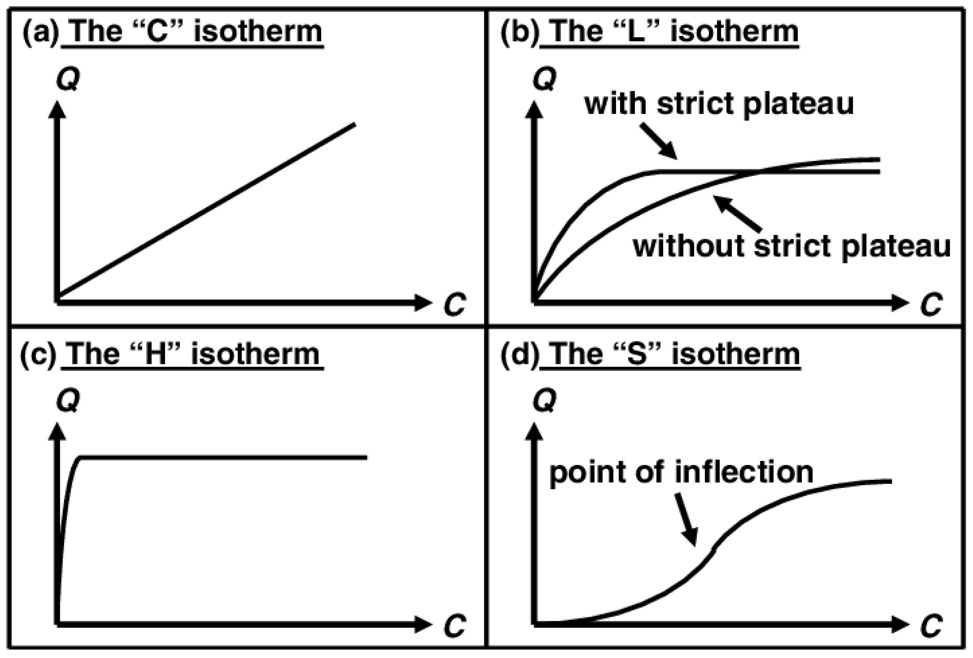
Table 1.
Screening tools and modelled processes.
| Model | Dimension | Flow | Transport | Biodegradation | Kinetics | Sorption | Cost |
|---|---|---|---|---|---|---|---|
| BioBalance Toolkit | 1D flow | Vad, S, S-S | 3D dispersion | +(AN) | F-O | + | Free |
| BIOCHLOR | 1D flow, 2D transport | S, S-S | 1D advection, 3D dispersion | + (AN) | F-O | + | Free |
| BIOSCREEN | 1D flow, 2D transport | S, S-S | 1D advection, 3D dispersion | + (AN, AE) | F-O, I | + | Free |
| CapSim | 1D flow | S, S-S, T | 1D transport | + | F-O | + | Free |
| CDISCO | 1D transport | S, S-S, | 1D transport, | - | F-O | + | Free |
| HSSM | 1D flow, 1D transport in vadose zone, 2D transport in saturated zone | Vad, S, S-S, T | 1D transport in Vad. zone, and 2D in saturated zone | - | - | - | Free |
| NAS | 1D flow, combined transport | S, S-S, T | 2D analytical 3D numerical | + (AN, AE) | F-O | + | Free |
| REMChlor | 1D flow, 2D transport | S, S-S | 1D advection, 3D dispersion | + (AN, AE) | F-O | + | Free |
| REMFuel | 1D flow, 2D transport | S, S-S | 1D advection, 3D dispersion | + (AN, AE) | Zero-O; F-O, M | + | Free |
| RT1D | 1D flow, 1D transport | S, S-S | 1D transport | + (AN, AE) | F-O, M, or other user-defined | + | Free |
| SourceDK | 1D | S, S-S | 1D advection and dispersion | + | F-O | + | Free |
Vad—vadose zone, S—saturated zone, S-S—steady state condition, T—transient condition, AN—anaerobic biodegradation, AE—Aerobic biodegradation, F-O—first order, I—instantaneous, M—Monod, M—Michelis–Menten.
Disclaimer/Publisher’s Note: The statements, opinions and data contained in all publications are solely those of the individual author(s) and contributor(s) and not of MDPI and/or the editor(s). MDPI and/or the editor(s) disclaim responsibility for any injury to people or property resulting from any ideas, methods, instructions or products referred to in the content. |
© 2024 by the authors. Licensee MDPI, Basel, Switzerland. This article is an open access article distributed under the terms and conditions of the Creative Commons Attribution (CC BY) license (https://creativecommons.org/licenses/by/4.0/).
Share and Cite
MDPI and ACS Style
Samborska-Goik, K.; Pogrzeba, M. A Critical Review of the Modelling Tools for the Reactive Transport of Organic Contaminants. Appl. Sci. 2024, 14, 3675. https://0-doi-org.brum.beds.ac.uk/10.3390/app14093675
AMA Style
Samborska-Goik K, Pogrzeba M. A Critical Review of the Modelling Tools for the Reactive Transport of Organic Contaminants. Applied Sciences. 2024; 14(9):3675. https://0-doi-org.brum.beds.ac.uk/10.3390/app14093675
Chicago/Turabian StyleSamborska-Goik, Katarzyna, and Marta Pogrzeba. 2024. "A Critical Review of the Modelling Tools for the Reactive Transport of Organic Contaminants" Applied Sciences 14, no. 9: 3675. https://0-doi-org.brum.beds.ac.uk/10.3390/app14093675
Note that from the first issue of 2016, this journal uses article numbers instead of page numbers. See further details here.