Estimating the Thermal Conductivity of Unsaturated Sand

Abstract

A modified parallel model for estimating the thermal conductivity of unsaturated sand was proposed in this study. The heat conduction in the solid phase of sand depends mainly on the form of contacts between solid particles, while water bridges at the particle contacts increase the contact areas and remarkably enlarge the transfer paths of heat conduction in sandy soils. However, the thermal conductivity of the solid particle itself (λ_s) cannot describe the influence of the form of contacts and water bridges on heat conduction through the solid phase. In this study, the equivalent thermal conductivity of the solid particle (λ_es) was presented which reflected the influence of the form of contacts and water bridges between particles under dry conditions or a low degree of saturation, respectively. The relationship between λ_es and degree of saturation was described by hyperbolic expression. The modified model was calibrated using measured values of the thermal conductivity from published datasets, including those for 41 types of sand from 15 studies. Numerical analyses of the temperature field of the energy pile were performed and validated against laboratory measurements. The results illustrated that the modified model was more applicable than the original model for predictions of sand thermal conductivity.

1. Introduction

In recent decades, with the development of energy engineering, soil science, and agroclimatology, the study of the thermal conductivity of soil (λ, Wm⁻¹°C⁻¹) has always occupied a crucial place in soil thermal property research [1,2,3]. As the direct impact factor in initial temperature changes of soil, the soil mechanical properties and soil ecosystem are affected by the temperature gradient distribution, which is associated with the thermal conductivity of soil [4].

A number of studies have been conducted on the experimental measurement of the thermal conductivity of soil. Smits et al. [5] measured the variation of four sand thermal conductivities λ with differences in porosity and found that λ was a function of moisture content under both transient drainage or drying and wetting conditions. Chen [6] published experimental results for the thermal conductivity λ of four kinds of quartz sands with different particle gradations by the transient thermal probe method. The thermal conductivity λ of sands tended to diminish with increasing porosity; in contrast, it increased with increasing moisture content. A series of thermal conductivity experiments was performed by Barry-Macaulay et al. [7], who tested six soils and three rocks from the region around Melbourne, Australia, and measured the impacts of moisture content, dry density, mineralogical composition, and particle size on the sample thermal conductivities. Zhao et al. [8] used the heat-pulse method to measure the thermal conductivity λ of six soils under wide ranges of moisture contents and bulk densities and proposed a new model that could accurately describe the trend of thermal conductivity λ. Therefore, the majority of the experimental research investigated the effects of physical characteristics, including water content, bulk and particle densities, compositional factors, and gradation, on thermal conductivity [9,10,11,12,13,14].

There are a variety of models that can predict the soil thermal conductivity λ. Three types of models can be distinguished in the present literature: theoretical, empirical, and mixture models [15]. Theoretical models were frequently derived from simplistic mathematical models and analyses based on heat transfer mechanisms [16], soil grain geometries [17,18], and other properties, e.g., dielectric permittivity. However, the theoretical models generally applied homogenization assumptions to consider the effective thermal property of a given component, and none of the theoretical models considered the microstructure of the soil [19]. The empirical soil thermal conductivity models were developed using datasets of experimental measurements of soil. Johansen [20] proposed a kr-Sr relationship between normalized thermal conductivity and soil physical properties, such as soil type, porosity, degree of saturation, and mineral component. Kersten [21] proposed an empirical model based on a series of laboratory measurements of 19 types of soils, and the empirical model described the relationships between thermal conductivity, moisture content, and dry density. However, empirical models are only persuasive for specific soils and lack a clear physical foundation because of differences between the physical properties of each natural soil [19].

The most common mixture models are based on classical mixing laws of the series thermal conductivity (STC) model and parallel thermal conductivity (PTC) model [19]. Compared to theoretical and empirical models, the advantages of mixing models are more obvious since they are based on the physical and heat transport properties of porous media [22]. Two basic mixture models, STC and PTC models, determine the volume percentage and thermal conductivity of each phase in media [14,23,24,25,26]. Nam et al. [27] developed a numerical model that combines a heat transport model and a heat exchanger model to predict the heat exchange rates for a ground source heat pump system. The PTC model was used for the estimation of thermal conductivity of soil in the numerical analysis. Bottarelli et al. [28] evaluated the application of a novel ground heat exchanger through numerical modeling to solve transient heat transfer, and the thermal conductivity of the mixed backfill materials was obtained by the PTC model. Chen et al. [29] proposed a numerical model of a vertical ground heat exchanger with the finite-volume method to evaluate the effects of thermal conductivity, volumetric heat capacity, temperature, and soil porosity, where the thermal conductivity of backfill materials was expressed as the PTC model. A mathematical model was developed to analyze the influence of unsaturated soil properties and groundwater flow on the performance of ground source heat pump systems by Li et al. [30], and the thermal conductivity of ground can be represented by the PTC model which was expressed as the sum of the thermal conductivity of each phase according to their volume fractions.

According to the above studies, the PTC model is still widely used in numerical analysis because it can reasonably describe the physical and heat conduction properties of soil. However, the prediction of the PTC model is not the most accurate. The reason for this was that the value calculated by the PTC model is based on the assumption that the components are superposed to form a multiphase mixture, but the form of contact between solid particles is not taken into consideration which has a significant effect on soil thermal conductivity [11,25,26]. Thus, the values of the calculation by the PTC model which presented the upper bound of the thermal conductivity of the soil generally overestimated the data [15]. It is necessary to develop a more accurate and comprehensive model of soil thermal conductivity based on the PTC model.

The aim of this study was to develop a modified model based on the PTC model to calculate the thermal conductivity λ of sand over a wide range of moisture contents from dry to saturated. The calculation steps of the modified model are presented. Based on the results, the performance of the modified model was validated by comparison with published datasets for a wide range of sand types. Finally, the modified model was used in the numerical analysis of the temperature field simulation, and the simulated and measured values were in good agreement.

2. Heat Transfer Mechanisms of Sand

As a kind of porous medium, the thermal properties of sand are determined by the volume fraction of each constituent material, such as soil particles, water, and air. Previous studies have revealed that conduction was generally the dominant heat transfer mechanism of sand produced by the presence of temperature gradients, and convection heat transfer undertook a significant role only in highly permeable soils. In this paper, the symbol λ refers to the thermal conductivity of sand.

The thermal conductivity of the solid phase is on average approximately 6 times and 200 times that of water and air, respectively. Specifically, for completely dry sand, or under great matric suction, heat is mainly conducted through the solid phase and restricted by contact points between solid particles. When the water content increases, the initial water is in the lowest energy state, and water menisci form near the particle contact region where they are the most stable [31,32]. In this paper, menisci are called transitory water bridges because the characteristic of the water bridge is connecting the gap between neighboring particles. The water bridges at the particle contacts increase the contact areas and thus remarkably enlarge the transfer paths of heat conduction in sand. Particle–particle conduction is altered to particle–water–particle conduction, which causes a rapidly increasing tendency in thermal conductivity, as shown in Figure 1. As the water content continues to increase, individual water bridges are gradually interconnected and form an evenly distributed water membrane coating on all particles. This phenomenon is generally referred to as the funicular regime, which is conducive to the further augmentation of the thermal conductivity of sand [33]. The contributions of particle–water–particle conduction in enhancing the thermal conductivity of sand achieve its maximum at this stage.

Unsaturated sand gradually tends to saturate with increasing moisture content. At this point, the heat transfer mechanism of sand changes from solid phase conduction to joint conduction by the solid and liquid phases, with continuously increasing thermal conductivity due to increasing water content. However, the rates of increase in thermal conductivity decrease gradually as the sand tends to full saturation. Hence, the curve of thermal conductivity, as shown in Figure 1, approaches a plateau, which indicates that the thermal conductivity of sand reached its maximum value λ_sat.

3. Model Development

3.1. Parallel Theoretical Models (Wiener Model)

Sand is considered a porous medium that is composed of air, water, and solids; the particles of sand have point contacts with their neighbors. Each sand has a unique mineral composition, size distribution of the solid phase, and geometry of the particle and pore structure, and those parameters have a significant influence on the thermal properties of the soil [34,35,36]. Furthermore, the water content in the pores of sand plays an important role. Consequently, it is difficult to assess whether a prediction accurately considers all these factors [37]. The proposed PTC model predicts the thermal conductivity of soil based on the volume fraction of the three phases, i.e., solid, liquid, and air, and the models are expressed as follows:

$${\mathsf{\lambda }}_{\mathrm{parallel}}=\sum {\mathsf{\varphi }}_i{\mathsf{\lambda }}_i={\mathsf{\varphi }}_s{\mathsf{\lambda }}_s+{\mathsf{\varphi }}_w{\mathsf{\lambda }}_w+{\mathsf{\varphi }}_a{\mathsf{\lambda }}_a$$

(1)

where λ_parallel is the thermal conductivities of the PTC model in the unfrozen state; ϕ_i is the volume fraction of component i, and ∑ϕ_i = 1; ϕ_s, ϕ_w, and ϕ_a and are the volume fractions of solid particles, water, and air, respectively; λ_i is the thermal conductivity of component i; λ_s is the solid thermal conductivity (2 to 8 Wm⁻¹°C⁻¹); λ_w and λ_a are the thermal conductivity of water (0.6 Wm⁻¹°C⁻¹) and air (0.02 Wm⁻¹°C⁻¹), respectively.

The PTC model has the advantage of using clearly defined concepts to estimate the thermal conductivity of soil. In general, the air volume, moisture content, and particle density are represented by selecting the two indexes, porosity n and degree of saturation S_r [38,39]. Thus, the PTC model is also expressed by:

$${\lambda }_{\mathrm{parallel}}=\left\{\begin{array}{cc}\left(1-n\right){\mathsf{\lambda }}_s+n{\mathsf{\lambda }}_a& S_r=0\\ \left(1-n\right){\mathsf{\lambda }}_s+n{S_r\mathsf{\lambda }}_w+n\left(1-S_r\right){\mathsf{\lambda }}_a& S_r\ne 0\end{array}\right.$$

(2)

However, the materials are made up of columns in the PTC model, and the heat conduction is constant at all points and the same in both phases, which depends on the thermal conductivity of each phase. The reason for the upper bound of the thermal conductivity of media was calculated by the PTC model based on the assumption that the components were superposed to form a multiphase mixture, but the form of contact between solid particles was not taken into consideration. Figure 2 indicates the comparison between measured values and calculated values from the PTC model; four examples were derived from the literature [6,8,40]. As shown in Figure 2, compared to the measured values, the PTC model gave an upper bound, and the results of the calculation generally overestimated the data. The estimated values of the PTC model showed a linear trend over a wide range of S_r; this tendency of the sand thermal conductivity did not correspond to the actual situation, which showed a nonlinear trend represented by the measured values. The maximum error in the calculated value of the PTC model occurred at S_r = 0 and gradually decreased according to the increase in S_r because the soil was treated as a continuum by the PTC model; broken and scattered particles were not considered.

3.2. Equivalent sand Particle Thermal Conductivity λ_es

When the sand is in a completely dry condition, conductive heat transfer is mainly controlled by contact between particles, which has been discussed previously. However, in the PTC model, the solid particle thermal conductivity λ_s is adopted to characterize the property of conductive heat transfer of the solid phase, which does not consider contacts between particles. Therefore, the influence of the contacts between particles could not be sufficiently reflected by the solid particle thermal conductivity λ_s. Then, the formation of water bridges among particles remarkably enlarges the transfer paths of heat conduction in sand so that the thermal conductivity of sand increases sharply when the sand is under low degrees of saturation. Similarly, the effect of water bridges cannot be adequately represented in λ_s. Thus, in this study, we proposed using the equivalent thermal conductivity of solid particles λ_es instead of solid particle thermal conductivity λ_s in the PTC model; this changed the PTC model to a nonlinear model, which was sufficient to present the effects of the contact features of particles and water bridges near the particle contacts.

Detailed derivations of the equivalent thermal conductivity of solid particle λ_es are included below. First, the measured value of the thermal conductivity of sand was determined by testing in the dry state, which contained the effect of contacts between particles. Then, by substituting the measured value in the left side of Equation (2), we obtained the formula by a simple transformation of variables:

$${\mathsf{\lambda }}_{\mathit{es}}={\mathsf{\lambda }}_{\mathit{es}}^{\mathit{dry}}=({\mathsf{\lambda }}_{\mathrm{measured}}-n{\mathsf{\lambda }}_a)/(1-n)\hspace{1em}{S}_r=0$$

(3)

where ${\mathsf{\lambda }}_{\mathit{es}}^{\mathit{dry}}$ is the equivalent thermal conductivity of solid particles in the completely dry state, which represents the thermal conductivity of the solid phase of sand affected by contacts between particles and is typically less than λ_s. Finally, the measured value of S_r ≠ 0 was substituted in the left side of Equation (2), which was determined by testing, and the formula was obtained as:

λ_es = [λ_measured − nS_rλ_w − n(1 − S_r) λ_a]/(1 − n) S_r ≠ 0

(4)

For example, with Sample A, Figure 3 indicates that the equivalent thermal conductivity of solid particle λ_es increased with S_r and was generally larger than the measured value of the sand thermal conductivity at the same S_r. The change in the trend of λ_es with S_r was consistent with the trend of the measured value. The λ_es at the low range of S_r increases rapidly on top of ${\mathsf{\lambda }}_{\mathit{es}}^{\mathit{dry}}$ and then goes into a stable region as S_r approaches saturation. When S_r ≠ 0, liquid in the pores exerts an effect on heat transfer, including increased contact area between particles, by the presence of a transitory water bridge at low S_r and heat conduction in liquid at higher S_r. As a result, the effects of liquid were not captured in ${\mathsf{\lambda }}_{\mathit{es}}^{\mathit{dry}}$. Figure 3 shows that λ_es was a function of S_r when S_r ≠ 0, and the relationship between λ_es and S_r was described by a hyperbolic expression. Thus, λ_es was expressed by the following equations:

$${\mathsf{\lambda }}_{\mathit{es}}={\mathsf{\lambda }}_{\mathit{es}}^{\mathit{dry}}+f(S_r)$$

(5)

$$f\left(S_r\right)=S_r/(A·{ S}_r+B)$$

(6)

where A and B are sand-dependent parameters.

The lower and upper limit conditions of Equation (5) are as follows:

Lower limit condition: S_r = 0 → ${\mathsf{\lambda }}_{\mathit{es}}={\mathsf{\lambda }}_{\mathit{es}}^{\mathit{dry}}$;

Upper limit condition: S_r = 1 → ${\mathsf{\lambda }}_{\mathit{es}}={\mathsf{\lambda }}_{\mathit{es}}^{\mathit{dry}}+1/(A+B)$.

Equations (5) and (6) were substituted into Equation (2), λ_s was replaced by λ_es, and the modified parallel thermal conductivity (MPTC) model was obtained:

$$\mathsf{\lambda }=\left\{\begin{array}{cc}\left(1-n\right){\mathsf{\lambda }}_{\mathit{es}}^{\mathit{dry}}+n{\mathsf{\lambda }}_a& S_r=0\\ \left(1-n\right)\left[{\mathsf{\lambda }}_{\mathit{es}}^{\mathit{dry}}+S_r/(A{· S}_r+B)\right]+n{S_r\mathsf{\lambda }}_w+n\left(1-S_r\right){\mathsf{\lambda }}_a& S_r\ne 0\end{array}\right.$$

(7)

3.3. A Mathematical Model of ${\mathsf{\lambda }}_{\mathit{es}}^{\mathit{dry}}$

The measures of thermal conductivity of dry sand were obtained from

Table A1. Summary of physical properties of sands.

No.	Sand	Texture	Particle Size Distribution (% Mass)			fq (%)	n (%)	ρs (g/cm3)	Literature Source
			Clay	Silt	Sand
1	Pozzolama	Loamy sand	3	26	71	0	0.44–0.5	2.75	[13]
2	L-soil (30)	Loamy sand	6	27	67	0	0.43	2.65	[34]
3	ON-04	Loamy sand	1	10	89	38	0.39	2.76	[11]
4	ON-06	Loamy sand	2	14	84	38	0.44	2.74	[11]
5	QC-01	Sand	2	5	93	35	0.43	2.72	[11]
6	BJ (20–30)	Sand	1	7	92	46	0.37	2.53	[50]
7	BJ (30–40)	Loamy sand	1	15	84	45	0.37	2.50	[50]
8	QC-02	Loamy sand	4	17	79	42	0.48	2.69	[11]
9	ON-03	Loamy sand	3	26	71	41	0.46	2.71	[11]
10	Limestone sand	Sand	0	0	100	40	0.27–0.39	2.74	[40]
11	Granite B	Sand	0	0	100	45	0.30	2.65	[51]
12	Anduo (10–20)	Loamy sand	3	16	81	45	0.46	2.65	[50]
13	Anduo (20–30)	Loamy sand	3	11	86	45	0.39	2.65	[50]
14	Anduo (30–40)	Loamy sand	8	23	69	45	0.30	2.65	[50]
15	PE-03	Loamy sand	2	14	84	54	0.41	2.66	[11]
16	MN-04	Loamy sand	4	15	81	61	0.47	2.71	[11]
17	SK-02	Loamy sand	6	27	67	61	0.45	2.70	[11]
18	SK-04	Loamy sand	3	14	83	67	0.42	2.68	[11]
19	SK-05	Loamy sand	4	28	68	63	0.45	2.68	[11]
20	Brighton sand	Loamy sand	20	19	61	63	0.39–0.49	2.59	[7]
21	Toyoura	Sand	0	0	100	75	0.38–0.40	2.63	[9]
22	NS-05	Loamy sand	2	13	85	72	0.40	2.66	[11]
23	Quartzite sand	Sand	0	0	100	80	0.34–0.38	2.65	[40]
24	Ottawa sand	Sand	0	0	100	100	0.34–0.36	2.70	[52]
25	Masonry sand	Sand	0	0	100	80	0.27–0.40	2.65	[40]
26	Sand-Kaolin-1	Sand	5	0	95	95	0.34–0.41	2.65	[12]
27	Sand-Kaolin-2	Sand	10	0	90	90	0.35–0.40	2.64	[12]
28	PS14-H	Sand	0	3	97	97	0.45	2.65	[8]
29	Silica sand	Sand	0	0	100	90	0.25–0.38	2.65	[40]
30	12/20 (tight)	Sand	0	0	100	99	0.31	2.65	[5]
31	12/20 (loose)	Sand	0	0	100	99	0.40	2.65	[5]
32	Sand	Sand	0	0	100	100	0.36–0.40	2.65	[12]
33	Sand-L	Sand	0	0	100	100	0.45	2.65	[8]
34	Sand-H	Sand	0	0	100	100	0.40	2.65	[8]
35	C-109	Sand	0	0	100	100	0.32–0.40	2.65	[9]
36	C-190	Sand	0	0	100	100	0.40	2.65	[9]
37	NS-04	Sand	0	0	100	100	0.36	2.66	[11]
38	Sample A	Loamy sand	5	27	68	100	0.40–0.49	2.65	[6]
39	Sample B	Sand	0	6	94	100	0.43–0.55	2.65	[6]
40	Sample C	Sand	0	6	94	100	0.43–0.55	2.65	[6]
41	Sample D	Loamy sand	13	27	60	100	0.35–0.47	2.65	[6]

in Appendix A and the correlation curve of ${\mathsf{\lambda }}_{\mathit{es}}^{\mathit{dry}}$ with porosity was plotted. Figure 4 shows that the relationship between ${\mathsf{\lambda }}_{\mathit{es}}^{\mathit{dry}}$ and porosity was linear based on Equation (8) (0.2 < n ≤ 0.5). As the porosity increased, ${\mathsf{\lambda }}_{\mathit{es}}^{\mathit{dry}}$ decreased because the thermal conductivity of the air phase was lower than that of the mineral composition. This was in accordance with the findings of previous research [41,42]. However, the main conductive mechanism of dry sand is contact conductance, and the effect of quartz content f_q was insignificant. Therefore, ${\mathsf{\lambda }}_{\mathit{es}}^{\mathit{dry}}$ correlated with porosity as follows:

$${\mathsf{\lambda }}_{\mathit{es}}^{\mathit{dry}} = -\mathit{kn} + \mathsf{\theta }$$

(8)

where k and θ are indeterminate coefficients that can be determined through experiments. From Equation (7), it can be concluded that the modified parallel model of dry sand is:

$$\mathsf{\lambda }=(1-n) (-\mathit{kn}+\mathsf{\theta })+n{\mathsf{\lambda }}_a\hspace{1em}{S}_r=0$$

(9)

The coefficients k and θ can be determined by fitting Equation (8) to the heat-pulse measurements. Figure 4 plots the ${\mathsf{\lambda }}_{\mathit{es}}^{\mathit{dry}}–$n values and the fitted lines, which are represented by dashed and solid lines. For completely dry sand, ${\mathsf{\lambda }}_{\mathit{es}}^{\mathit{dry}}$ was affected only by the porosity of the sand.

First, measurements of dry sand thermal conductivity should be made for no fewer than three groups of sand with different porosities. Next, ${\mathsf{\lambda }}_{\mathit{es}}^{\mathit{dry}}$ corresponding to the test groups is calculated based on Equation (3). In this way, the coefficients k and θ can be obtained by fitting ${\mathsf{\lambda }}_{\mathit{es}}^{\mathit{dry}}–$n values according to Equation (8) and used to prepare for the subsequent stages of determination of parameters A and B in Equation (6).

3.4. Determination of Parameters A and B

The physical characteristics of samples, such as grain size distribution, particle and bulk density, and porosity should be defined before laboratory thermal conductivity experiments. The determination of parameters A and B can be accomplished using the following steps. First, at a constant temperature, which is controlled within the range of 20~30 °C, the dry thermal conductivity λ_dry of the samples is measured by the transient method, and ${\mathsf{\lambda }}_{\mathit{es}}^{\mathit{dry}}$ is calculated based on Equation (3). ${\mathsf{\lambda }}_{\mathit{es}}^{\mathit{dry}}$ is a function of sand porosity as discussed previously. Then, the sample thermal conductivity λ is measured for different S_r values under identical settings. The spans of S_r elected in the test should be larger than 15%, and the magnitudes of selected S_r should cover above 80%. A series of λ_es values for different S_r are calculated via Equation (4). Finally, the relationship of the proposed function f(S_r) between λ_es (S_r ≠ 0) and S_r can be described by a hyperbolic expression, and the parameters A and B in the hyperbolic expression can be determined through nonlinear regression analysis based on the calculated λ_es.

Figure 5 shows that the parameters A and B of the four samples are determined by nonlinear regression analysis, which is performed by a hyperbola. For each sample, the hyperbolic expression fit of λ_es to S_r can better describe the increase in λ_es with S_r. The growth trends of λ_es in the form of a hyperbolic curve are dramatic, especially when S_r varies from 0 to 30%, and then enters a stable region as S_r is over 40%. After the series of steps above, substituting the coefficients including ${\mathsf{\lambda }}_{\mathit{es}}^{\mathit{dry}}$ and parameters A and B of f(S_r) into Equation (7), the full MPTC model can be obtained.

3.5. Model Validation

It is therefore necessary to obtain dependable experimental data to better evaluate the thermal conductivity model. Thus, the experimental data comply with several important criteria: (1) the experimental results are measured on soil samples with the transient method and shown to be accurate and reproducible; (2) cohesionless soil is a collection of objects with a detailed description of the grain size distribution, such as the contents of clay, silt, and sand; (3) the detailed properties of specimens are reported, including grain size distribution, quartz mineral content, texture of sand, saturation degree S_r, porosity ratio n, and particle density ρ_s; (4) the ambient temperature of the experiment is within the range from 20~30 °C; (5) each selected experimental dataset should contain a wide range of S_r from dryness to saturation. Table A1 in Appendix A shows that a total of 41 sands were collected from 15 sources published in the literature.

For each referenced sand, at least four measurements of thermal conductivity were made with the variation of S_r including dry and saturated. Thus, the 41 sands from the literature were able to fulfil the condition of building an independent MPTC model for each sand. The framework of building the MPTC model is shown in Figure 6, and the predicted values of thermal conductivity for each referenced sand calculated by the independent MPTC model were obtained, which corresponded to S_r in the test. From the above findings, it was concluded that for constructing f(S_r), as least three independent sets of thermal conductivity experiments of the sample are performed under dry conditions and two different degrees of saturation conditions. Figure 7 shows the comparison of the calculated thermal conductivity values of sand calculated by the MPTC model with measurements of the 41 sands from the literature, as presented in Table A1 of Appendix A. Figure 7 shows that most of the thermal conductivities calculated using the MPTC model were in good agreement with the experimental data. Of the errors, 86% were less than 10% of the calculated values, which verified the accuracy and effectiveness of the proposed model.

4. Numerical Models with the MPTC Model

The final goal of this paper was to use a numerical approach to verify the applicability of the MPTC model. For this purpose, numerical models were used to evaluate the temperature field of the energy pile for various degrees of sand saturation. The results of the numerical model were compared against a series of laboratory experiments. Afterwards, we extended the numerical model to account for the sand temperature profile, and we used a numerical model associated with the MPTC model to evaluate the temperature field of sand for saturation conditions.

The indoor test employed to validate the applicability of the MPTC model was derived from Akrouch [43]. The indoor test included a series of sand thermal conductivity tests and temperature field tests of energy piles of unsaturated sands. First, a total of 12 groups under different S_r (0.015, 0.111, 0.188, 0.245, 0.311, 0.421, 0.480, 0.590, 0.715, 0.840, and two groups of 1.000) in thermal conductivity tests of the same sand with an average value around γ_d = 14.5 kN/m³ and n = 0.45 were included; secondly, with respect to temperature field tests, the energy pile was embedded inside a square wooden box with dimensions of 1.2 × 1.2 × 0.25 m filled with sand with diameters of 300 mm and 400 mm. Two PVC pipes in the pile served as the heating source; water inside the pipes remained at a constant value of 37 °C. All experimental procedures were performed in a room maintained at a constant temperature of 21 °C. Different degrees of saturations of sand (0.015, 0.188, 0.311, 0.480, 0.715, and 1.000) were adopted, and each experiment was conducted for 48 h. Sheets of foam insulation enclosed the top and bottom of the wooden box to prevent heat transfer in the vertical direction, and the tests were regarded as 2D plane heat conduction because an effective temperature gradient was not present along the height of the wooden box. In this study, the simulation only addressed an energy pile with a diameter of 300 mm.

4.1. Comparison between Measured and Calculated Values of Thermal Conductivity of Sand

One of those thermal conductivity tests included a sand with S_r = 0.015, which was regarded as the dry condition. Consequently, in accordance with the derivation condition of the MPTC model for the sand, the parameters A and B of f(S_r) were accurately determined. Then, the complete MPTC model for predicting the thermal conductivity of test sand was obtained. Figure 8 plots the sand thermal conductivity values calculated using the MPTC model against the values under different S_r values that were measured in the laboratory experiment [43]; there was satisfactory agreement between the calculated and experimental values over the range of S_r. The fitted curve of the hyperbolic expression for f(S_r) gave an accurate representation as a function of S_r.

4.2. Energy Pile Model

The finite element software PLAIXS 2D (V21.02) was employed for the numerical analyses. This software was able to deal with the temperature profile of soil formation and to couple and analyze the effect of temperature on the mechanics of soil. However, the major objective of this paper was to control the heat conduction of sandy soil by thermal properties; mechanical effects were ignored. Figure 9 shows the 2D model and mesh adopted for numerical analysis from the above laboratory energy pile tests. No heat protection measures were adopted at the perimeters for the wooden box in laboratory tests. Thus, the temperature boundary condition of the model and initial temperature for all materials were assumed to be equal to room temperature (21 °C). Notably, the influence of moisture migration on heat conduction in sand during the numerical simulation was neglected.

Since the thermal properties of the energy pile were lacking, in the numerical analysis, the pile was intended to be replaced by a circular temperature boundary that provided the heat source for the whole model. The laboratory experiments presented the temperatures of point B, C, D, E, F, and G. The detailed locations of those points are shown in Figure 9; among them, points B and E were located at the surface of the pile, and thus the temperature at points B and E represented the temperatures of different positions of the pile surface.

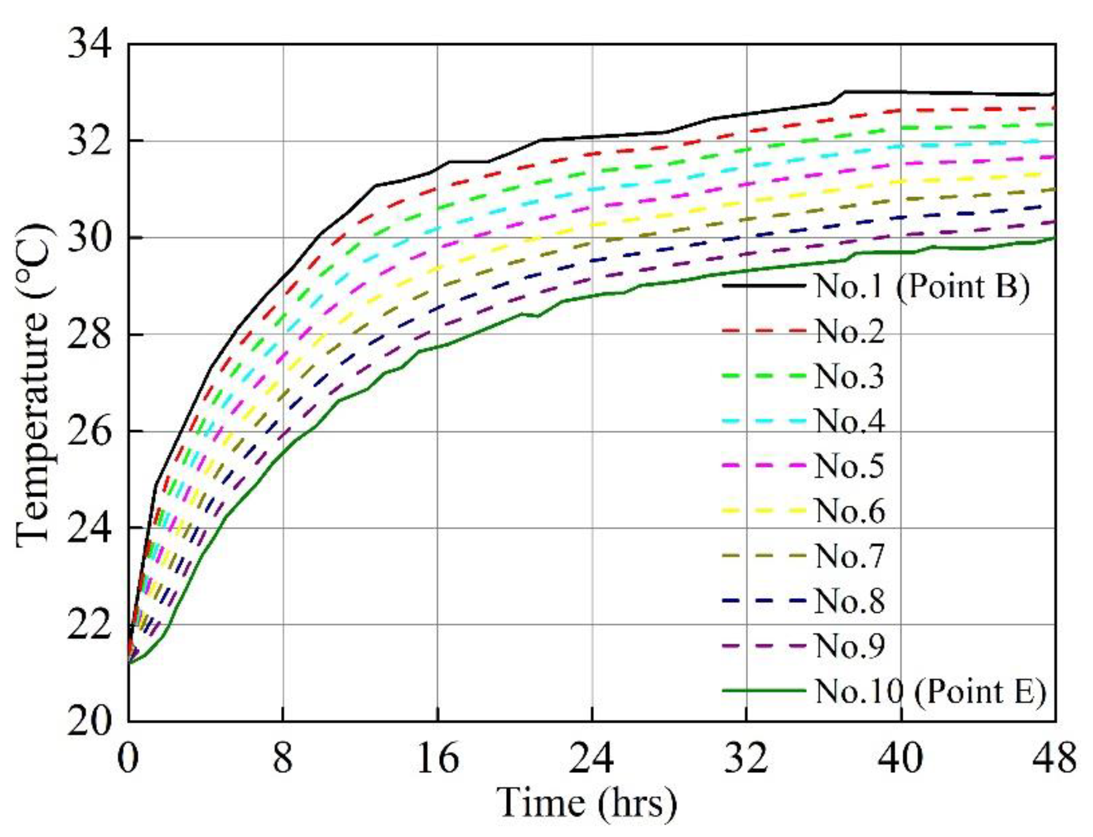
A discrete approach was used to simulate the temperature variation from point B to point E in the numerical analysis. First, the temperature variation from point B to point E was assumed to be a linear change along the circular temperature boundary. Then, the model was built with 2D axisymmetric geometry; thus, we took the temperature boundary of one quarter section as an example. As illustrated in Figure 10, the quarter circular temperature boundary was divided into 10 equal parts, and the temperature values at points B and E were adopted for parts 1 and 10, respectively. Finally, the value of the temperature difference between points B and E was divided into eight parts, which are shown in Figure 11 and correspond to the other eight parts of the discrete temperature boundary. This discrete approach was generalized to the entire circular temperature boundary to efficiently simulate the temperature variation along the circular temperature boundary.

4.3. Discussion of Volumetric Heat Capacity

The volumetric heat capacity (ρc) of soil is another of the most important parameters in a proper simulation of the temperature field of the ground surface and subsurface formation, which describes how well the soil stores heat. However, the volumetric heat capacity of sand could not be obtained from the literature because not enough specific details were given. The value of the volumetric heat capacity of sand selected for numerical simulation is discussed in the following paragraphs.

The volumetric heat capacity of soil was calculated from the sum of the heat capacities of the soil constituents through many trials and theoretical derivations [44,45,46,47]. Thus,

ρc = ρ_s c_s ϕ_s + ρ_w c_w ϕ_w + ρ_a c_a ϕ_a

(10)

where ρ is the density (kg m⁻³), c is the specific heat (kJ kg⁻¹ °C⁻¹), and ϕ is the volume fraction of the component; the subscripts s, w, and a indicate the soil, water, and air constituents, respectively, where ϕ_i =$\frac{V_{\mathrm{i}}}{V}$, and Equation (10) is given by:

$$\mathsf{\rho }c=\frac{V_{\mathrm{s}}}{V}{\mathsf{\rho }}_{\mathrm{s}} c_{\mathrm{s}}+\frac{V_{\mathrm{w}}}{V} {\mathsf{\rho }}_{\mathrm{w}}{c}_{\mathrm{w}}+\frac{V_{\mathrm{a}}}{V} {\mathsf{\rho }}_{\mathrm{a}}{\mathit{c}}_{\mathrm{a}}$$

(11)

since the porosity n and degree of saturation S_r are given by n = $\frac{V_{\mathrm{v}}}{V}$, and S_r = $\frac{V_{\mathrm{w}}}{V_{\mathrm{v}}}$, respectively. Equation (11) can be rewritten in the form:

$$\mathsf{\rho }c=\left(1- n\right) {\mathsf{\rho }}_{\mathrm{s}}{c}_{\mathrm{s}}+n S_{\mathrm{r}} {\mathsf{\rho }}_{\mathrm{w}}{c}_{\mathrm{w}}+n (1-S_{\mathrm{r}}) {\mathsf{\rho }}_{\mathrm{a}}{c}_{\mathrm{a}}$$

(12)

The values of the specific heat of the water and air were taken as 4.18 kJ kg⁻¹ °C⁻¹ and 1.00 kJ kg⁻¹ °C⁻¹, respectively. Generally, the value of c_s for clay was 1.10 kJ kg⁻¹ °C⁻¹ and 0.90 kJ kg⁻¹ for sand particles [48,49]. For that reason, five typical values of specific heat were selected (0.70, 0.80, 0.90, 1.00, and 1.10 kJ kg⁻¹ °C⁻¹) to discuss the influence of volumetric heat capacity on the temperature field of sand particles. The other parameters remained constant, including porosity n (0.45), ρ_s (2.65 kg/m³), and ρ (1.45 kg/m³). The numerical analyses of thermal conductivities of sand used the results of Section 4.1 and employed the model presented in Section 4.2. Among them, point C was taken as an example for the following analysis, and the temperature curves of point B were employed.

Figure 12 illustrates that the value adopted for the specific heat of sand particles had little influence on the variation in the temperature of the numerical analysis. A small amount of the variance in the results across the studies occurred when S_r = 0, and the differences decreased with increasing S_r. The reason was because water has a greater specific heat than sand particles and air, and water had a dominant effect on the volumetric heat capacity of the sand because the sand had large pores. Thus, the value of c_s for sand particles was selected to be 0.90 kJ kg⁻¹, and it was feasible in the numerical analysis.

4.4. Assessment of the MPTC Model

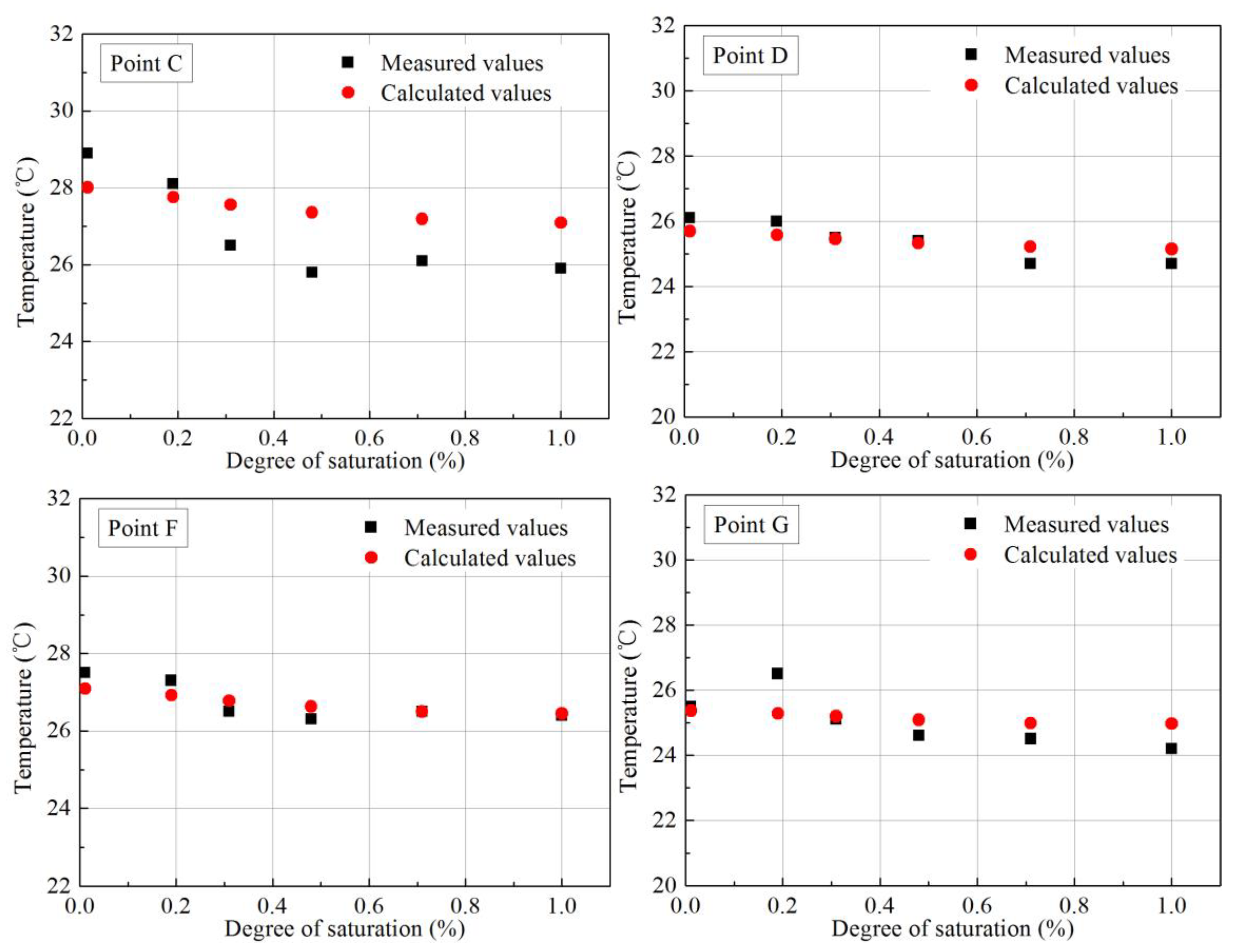
Figure 13 shows that most of the calculated values of temperature and the thermal conductivity of sand calculated by the MPTC model agreed well with the laboratory experimental data. However, a few slight deviations between the calculated and measured values were observed, especially for point C, for two reasons. First, the degree of saturation of sand remained constant for each group, but the spatial distribution of water in sand was altered during the experiment due to temperature gradients that caused moisture migration. However, the effect of moisture migration on heat conduction was not considered in the numerical simulation. Second, the porosity of the sand (n = 0.45) adopted in the numerical model was an average value, and the porosities of the samples in the experiments ranged from 0.44 to 0.47. Even so, the results of the comparison were convincing. In addition, the trends of temperature decreasing with increasing S_r were observed in the simulation, and they were consistent with the trend in the experimental data. Thus, the proposed model had sufficient precision for computing believable predictions, and the thermal conductivity of sand with different S_r can be evaluated by the MPTC model.

5. Conclusions

In this study, we developed a modified parallel model for estimating sand thermal conductivity with a wide range of moisture contents. We presented the equivalent thermal conductivity of solid particles λ_es and proposed a functional relationship between λ_es and S_r when S_r ≠ 0. The following conclusions can be drawn:

When S_r = 0, a back-extrapolation through the PTC model based on measurements was used to calculate ${\mathsf{\lambda }}_{\mathit{es}}^{\mathit{dry}}$. Compared to the solid particle thermal conductivity λ_s, the equivalent thermal conductivity of the solid particle λ_es sufficiently reflected the influence of contact between particles under dry conditions.

A simple hyperbolic relationship was applied to describe f(S_r), which presented the functional relationship between λ_es and S_r when S_r ≠ 0. Therefore, the complete form of λ_es was illustrated as the sum of ${\mathsf{\lambda }}_{\mathit{es}}^{\mathit{dry}}$ and f(S_r).

Comparisons between calculated values of sand thermal conductivity by the MPTC model and measurements of 41 sands from previous studies published in the literature indicated that the MPTC model was in good agreement with the experimental data.

To illustrate the utility and practicality of the MPTC model, the model was used in the numerical analysis of temperature field simulations, and the results indicated good agreement between the numerical and measured temperature values.

References

- Preene, M.; Powrie, W. Ground energy systems: From analysis to geotechnical design. Géotechnique 2009, 59, 261–271. [Google Scholar] [CrossRef]
- Choo, J.; Kim, Y.J.; Lee, J.H.; Yun, T.S.; Lee, J.; Kim, Y.S. Stress-induced evolution of anisotropic thermal conductivity of dry granular materials. Acta Geotech. 2013, 8, 91–106. [Google Scholar] [CrossRef]
- Bauer, S.; Urquhart, A. Thermal and physical properties of reconsolidated crushed rock salt as a function of porosity and temperature. Acta Geotech. 2016, 11, 913–924. [Google Scholar] [CrossRef]
- Nkongolo, N.V.; Johnson, S.; Schmidt, K.; Eivazi, F. Greenhouse gases fluxes and soil thermal properties in a pasture in central Missouri. J. Environ. Sci. 2010, 22, 1029–1039. [Google Scholar] [CrossRef] [PubMed]
- Smits, K.M.; Sakaki, T.; Limsuwat, A.; Illangasekare, T.H. Thermal conductivity of sands under varying moisture and porosity in drainage–wetting cycles. Vadose Zone J. 2010, 9, 172–180. [Google Scholar] [CrossRef]
- Chen, S.X. Thermal conductivity of sands. Heat Mass Transf. 2008, 44, 1241–1246. [Google Scholar] [CrossRef]
- Macaulay, D.B.; Bouazza, A.; Singh, R.M.; Wang, B.; Ranjith, P.G. Thermal conductivity of soils and rocks from the Melbourne (Australia) region. Eng. Geol. 2013, 2013, 131–138. [Google Scholar] [CrossRef]
- Zhao, Y.; Si, B.C.; Zhang, Z.H.; Li, M.; He, H.L.; Hill, R.L. A new thermal conductivity model for sandy and peat soils. Agric. For. Meteorol. 2019, 274, 95–105. [Google Scholar] [CrossRef]
- Tarnawski, V.R.; Momose, T.; Leong, W.H.; Bovesecchi, G.; Coppa, P. Thermal conductivity of standard sands. Part I. dry-state conditions. Int. J. Thermophys. 2009, 30, 949–968. [Google Scholar] [CrossRef]
- Pei, W.; Yu, W.; Li, S.; Zhou, J. A new method to model the thermal conductivity of soil-rock media in cold regions: An example from permafrost regions tunnel. Cold Reg. Sci. Technol. 2013, 95, 11–18. [Google Scholar] [CrossRef]
- Tarnawski, V.R.; Momose, T.; McCombie, M.L.; Leong, W.H. Canadian field soils III. thermal-conductivity data and modeling. Int. J. Thermophys. 2014, 36, 119–156. [Google Scholar] [CrossRef]
- Zhang, N.; Yu, X.B.; Pradhan, A.; Puppala, A.J. A new generalized soil thermal conductivity model for sand–kaolin clay mixtures using thermo-time domain reflectometry probe test. Acta Geotech. 2017, 12, 739–752. [Google Scholar] [CrossRef]
- McCombie, M.L.; Tarnawski, V.R.; Bovesecchi, G.; Coppa, P.; Leong, W.H. Thermal Conductivity of Pyroclastic Soil (Pozzolana) from the Environs of Rome. Int. J. Thermophys. 2016, 38, 21. [Google Scholar] [CrossRef]
- Firat, M.E.O. Experimental study and modelling of the thermal conductivity of frozen sandy soil at different water contents. Measurement 2021, 181, 109586. [Google Scholar] [CrossRef]
- Barry-Macaulay, D.; Bouazza, A.; Wang, B.; Singh, R.M. Evaluation of soil thermal conductivity models. Can. Geotech. J. 2015, 52, 1892–1900. [Google Scholar] [CrossRef]
- Carson, J.K.; Lovatt, S.J.; Tanner, D.J.; Cleland, A.C. Thermal conductivity bounds for isoptropic, porous materials. Int. J. Heat Mass Transf. 2005, 48, 2150–2158. [Google Scholar] [CrossRef]
- De Vries, D.A. Thermal properties of soils. In Physics of Plant Environment; North-Holland Publishing Corporation: Amsterdam, The Netherlands, 1963; pp. 210–235. [Google Scholar]
- Likos, W.J. Pore-scale model for thermal conductivity of unsaturated sand. Geotech. Geol. Eng. 2013, 33, 179–192. [Google Scholar] [CrossRef]
- Dong, Y.; McCartney, J.S.; Lu, N. Critical review of thermal conductivity models for unsaturated soils. Geotech. Geol. Eng. 2015, 33, 207–221. [Google Scholar] [CrossRef]
- Johansen, O. Thermal Conductivity of Soils. Ph.D. Thesis, University of Trondheim, Trondheim, Norway, 1977. [Google Scholar]
- Kersten, M.S. Laboratory Research for the Determination of the Thermal Properties of Soils; Bulletin No. 28; University of Minnesota Engineering Experiment Station: Minneapolis, MN, USA, 1949. [Google Scholar]
- Maroulis, Z.B.; Drouzas, A.E.; Saravacos, G.D. Modeling of thermal conductivity of Granular Starches. J. Food Eng. 1990, 11, 225–271. [Google Scholar] [CrossRef]
- Wiener, O. Die throrie des Mischkorpers für das Feld der Statonären Stromüng. I. Die Mittelwertsatze für Kraft, Polarisation und Energie. Der Abh. Der Math. -Phys. Kl. Der Königl Sachs. Ges. Der Wiss. 1912, 32, 509–604. [Google Scholar]
- Bi, J.; Zhang, M.; Chen, W.; Lu, J.; Lai, Y. A new model to determine the thermal conductivity of fine-grained soils. Int. J. Heat Mass Transf. 2018, 123, 407–417. [Google Scholar] [CrossRef]
- Bi, J.; Zhang, M.; Lai, Y.M.; Pei, W.S.; Lu, J.G.; You, Z.L.; Li, D.W. A generalized model for calculating the thermal conductivity of freezing soils based on soil components and frost heave. Int. J. Heat Mass Transf. 2020, 150, 119166. [Google Scholar] [CrossRef]
- Li, K.Q.; Li, D.Q.; Chen, D.H.; Gu, S.X.; Liu, Y. A generalized model for effective thermal conductivity of soils considering porosity and mineral composition. Acta Geotech. 2021, 16, 3455–3466. [Google Scholar] [CrossRef]
- Nam, Y.J.; Ooka, R.; Hwang, S. Development of a numerical model to predict heat exchange rates for a ground-source heat pump system. Energy Build. 2008, 40, 2133–2140. [Google Scholar] [CrossRef]
- Bottarelli, M.; Bortoloni, M.; Su, Y.H.; Yousif, C.; Aydin, A.A.; Georgiev, A. Numerical analysis of a novel ground heat exchanger coupled with phase change materials. Appl. Therm. Eng. 2015, 88, 369–375. [Google Scholar] [CrossRef]
- Chen, S.Y.; Mao, J.F.; Han, X. Heat transfer analysis of a vertical ground heat exchanger using numerical simulation and multiple regression model. Energy Build. 2016, 129, 81–91. [Google Scholar] [CrossRef]
- Li, C.F.; Cleall, P.J.; Mao, J.F.; Munoz-Criollo, J.J. Numerical simulation of ground source heat pump system considering unsaturated soil properties and groundwater flow. Appl. Therm. Eng. 2018, 139, 307–316. [Google Scholar] [CrossRef]
- Ewing, R.; Horton, R. Thermal conductivity of a cubic lattice of spheres with capillary bridges. J. Phys. D Appl. Phys. 2007, 40, 4959–4965. [Google Scholar] [CrossRef]
- Lu, N.; Zeidman, B.D.; Lusk, T.M.; Willson, C.S.; Wu, D.T. A monte carlo paradigm for capillarity in porous media. Geophys. Res. Lett. 2010, 37, L23402. [Google Scholar] [CrossRef]
- Lu, N.; Dong, Y. Closed-form equation for thermal conductivity of unsaturated soils at room temperature. J. Geotech. Geoenviron. Eng. 2015, 141, 04015016. [Google Scholar] [CrossRef]
- Campbell, G.S.; Jungbauer, J.D.; Bidlake, W.R.; Hungerford, R.D. Predicting the effect of temperature on soil thermal conductivity. Soil Sci. 2006, 158, 307–313. [Google Scholar] [CrossRef]
- Côté, J.; Konrad, J.M. A generalized thermal conductivity model for soils and construction materials. Can. Geotech. J. 2005, 42, 443–458. [Google Scholar] [CrossRef]
- Zhang, N.; Wang, Z.Y. Review of soil thermal conductivity and predictive models. Int. J. Therm. Sci. 2017, 117, 172–183. [Google Scholar] [CrossRef]
- Abu-Hamdeh, N.H.; Reeder, R. Soil thermal conductivity: Effects of density, moisture, salt concentration, and organic matter. Soil Sci. Soc. Am. J. 2000, 64, 1285–1290. [Google Scholar] [CrossRef]
- Mcgaw, R. Heat Conduction in Saturated Granular Materials; Specical Rep. No. 103; Highway Research Board: Washington, DC, USA, 1969; pp. 131–144. [Google Scholar]
- Hadley, G.R.; Mcvey, D.F.; Morin, R. Theophysical properties of deep ocean sediments. Mar. Geotech. 1984, 5, 257–295. [Google Scholar] [CrossRef]
- Sohn, B.H. Thermal conductivity measurement of sand-water mixtures used for backfilling materials of vertical boreholes or horizontal trenches. Korean J. Air Cond. Refrig. Eng. 2008, 20, 342–350. [Google Scholar]
- He, H.; Zhao, Y.; Dyck, M.F.; Si, B.; Jin, H.; Lv, J.L.; Wang, J.X. A modified normalized model for predicting effective soil thermal conductivity. Acta Geotech. 2017, 12, 1281–1300. [Google Scholar] [CrossRef]
- Lu, S.; Ren, T.; Gong, Y.S.; Horton, R. An Improved Model for Predicting Soil Thermal Conductivity from Water Content at Room Temperature. Soil Sci. Soc. Am. J. 2010, 71, 8–14. [Google Scholar] [CrossRef]
- Akrouch, G.A.; Sanchez, M.; Briaud, J.L. An experimental, analytical and numerical study on the thermal efficiency of energy piles in unsaturated soils. Comput. Geotech. 2015, 71, 207–220. [Google Scholar] [CrossRef]
- Bristow, K.L.; White, R.D.; Kluitenberg, G.J. Comparison of single and dual probes for measuring soil thermal properties with transient heating. Aust. J. Soil Res. 1994, 32, 447–464. [Google Scholar] [CrossRef]
- Rees, S.W.; Zhou, Z.; Thomas, H.R. Ground heat transfer: A numerical simulation of a full-scale experiment. Build. Environ. 2007, 42, 1478–1488. [Google Scholar] [CrossRef]
- Choi, J.C.; Lee, S.R.; Lee, D.S. Numerical simulation of vertical ground heat exchangers: Intermittent operation in unsaturated soil conditions. Comput. Geotech. 2011, 38, 949–958. [Google Scholar] [CrossRef]
- Wang, Y.T.; Liu, Y.Q.; Cui, Y.; Guo, W.C.; Lv, J.S. Numerical simulation of soil freezing and associated pipe deformation in ground heat exchangers. Geothermics 2018, 74, 112–120. [Google Scholar] [CrossRef]
- Bristow, K.L. Measurement of thermal properties and water content of unsaturated sandy soil using dual-probe heat-pulse probes. Agric. For. Meteorol. 1998, 89, 75–84. [Google Scholar] [CrossRef]
- Abu-Hamdeh, N.H. Thermal properties of soils as affected by density and water content. Biosyst. Eng. 2003, 86, 97–102. [Google Scholar] [CrossRef]
- Chen, Y.Y.; Yang, K.; Tang, W.J.; Qin, J.; Zhao, L. Parameterizing soil organic carbon’s impacts on soil porosity and thermal parameters for Eastern Tibet grasslands. Sci. China Earth Sci. 2012, 55, 1001–1011. [Google Scholar] [CrossRef]
- Côté, J.; Konrad, J.M. Thermal conductivity of base-course materials. Can. Geotech. J. 2005, 42, 61–78. [Google Scholar] [CrossRef]
- Park, S.; Hartley, J. A model for prediction of the effective thermal conductivity of granular materials with liquid binder. KSME J. 2016, 6, 88–94. [Google Scholar] [CrossRef]
Figure 1.
General relationship between soil thermal conductivity and degree of saturation.
Figure 2.
Comparison between measured and PTC-model-calculated values.
Figure 4.
Relationship between and n.
Figure 5.
Parameters of f(Sr) are determined by nonlinear regression analysis.
Figure 6.
Calculation steps for evaluation of sand thermal conductivity by MPTC model.
Figure 7.
Comparison between measured values and calculated values by MPTC model.
Figure 8.
Comparison between measured values and calculated values. The measured values are the experimental data from the literature [43]; the calculated values are calculated by MPTC model based on the measured values.
Figure 9.
The 2D model and mesh for numerical analysis.
Figure 10.
The discrete quarter circular temperature boundary.
Figure 11.
Temperature curves of discrete circular temperature boundary.
Figure 12.
The effect of specific heat of sand particles.
Figure 13.
Temperature values of calculated against measured values.
Disclaimer/Publisher’s Note: The statements, opinions and data contained in all publications are solely those of the individual author(s) and contributor(s) and not of MDPI and/or the editor(s). MDPI and/or the editor(s) disclaim responsibility for any injury to people or property resulting from any ideas, methods, instructions or products referred to in the content. |
© 2024 by the authors. Licensee MDPI, Basel, Switzerland. This article is an open access article distributed under the terms and conditions of the Creative Commons Attribution (CC BY) license (https://creativecommons.org/licenses/by/4.0/).
Share and Cite
MDPI and ACS Style
Liu, X.; Gao, Y.; Li, Y. Estimating the Thermal Conductivity of Unsaturated Sand. Appl. Sci. 2024, 14, 3673. https://0-doi-org.brum.beds.ac.uk/10.3390/app14093673
AMA Style
Liu X, Gao Y, Li Y. Estimating the Thermal Conductivity of Unsaturated Sand. Applied Sciences. 2024; 14(9):3673. https://0-doi-org.brum.beds.ac.uk/10.3390/app14093673
Chicago/Turabian StyleLiu, Xuejun, Yucong Gao, and Yanjun Li. 2024. "Estimating the Thermal Conductivity of Unsaturated Sand" Applied Sciences 14, no. 9: 3673. https://0-doi-org.brum.beds.ac.uk/10.3390/app14093673
Note that from the first issue of 2016, this journal uses article numbers instead of page numbers. See further details here.