Clustering-Based Classification of Polygonal Wheels in a Railway Freight Vehicle Using a Wayside System

Abstract

Polygonal wheels are one of the most common defects in train wheels, causing a reduction in comfort levels for passengers and a higher degradation of vehicle and track components. With the aim of contributing to the safety and reliability of railway transport, this paper presents the development of an innovative methodology for classifying polygonal wheels based on a wayside system. To achieve that, a numerical train-track interaction model was adopted to simulate the passage of a freight train over a virtual wayside monitoring system composed of a set of accelerometers installed on the rails. Then, the acquired acceleration time series was transformed to a frequency domain using a Fast Fourier transform (FFT), and on this data, damage-sensitive features were extracted. The features based on Principal Component Analysis (PCA) showed great sensitivity to the harmonic order, while the ones based on Continuous Wavelet Transform (CWT) model showed great sensitivity to the defect amplitude. One step further, all features are merged using the Mahalanobis distance in order to obtain a damage index strongly correlated with the polygonal defect. Finally, a cluster analysis allowed the automatic classification of polygonal wheels, according to the harmonic order (harmonic-based) and defect amplitude (amplitude-based). The proposed methodology demonstrated high efficiency in identifying different types of polygonal wheels using a minimum layout of two sensors.

1. Introduction

The interaction between the wheel and the rail gives rise to diverse forms of out-of-round wear on rail vehicle wheels. Operational wear on these wheels can manifest in various types, with the nature of the wear being influenced by the characteristics of the wheel–rail contact forces. Wheel wear can exhibit either uniform patterns or irregular ones [1], with irregular wear comprising both local and continuous wear. Local wear typically results from braking or worn-out treads [2], whereas continuous wear is commonly attributed to polygonization or corrugation [3]. These defects promote negative effects on both the vehicle and the track, increasing maintenance costs. From a railway safety point of view, wheel defects are one of the main causes of accidents, decreasing the reliability of this mode of transport [4].

Polygonal wheels are one of the most common defects in the railway wheel and consist of a periodic variation of the radius of the wheel along the circumference. Its wheel profile results from the superposition of several waves of harmonics characterized by a dominant harmonic order [5]. According to Peng et al. [6], when the amplitude of the defect assumes values above 0.2 mm and wavelengths between 140 mm and the wheel circumference, it is a polygonal wheel defect; otherwise, when the wavelength assumes values between 30 and 80 mm, it is considered a corrugation. The excitation frequencies it promotes cause a large fluctuation in the contact forces between the vehicle and the track, resulting in increased vibrations in the system [7,8]. Polygonal wheels increase the risk of rail breaks, sleeper and track fixing device cracking, axle damage, bearing damage, etc. [9]. It also increases the noise emissions inside and outside the vehicle, decreasing the comfort levels [10]. Depending on the vehicle’s characteristics and the type of harmonic order present in a polygonal wheel, the frequency excited by the polygonal damage may cause a resonance effect [11,12]. Thus, it is desirable to continuously monitor the health status of the wheels to prevent this defect.

To monitor the condition of railway systems in service, two approaches are usually used on-board and wayside. These systems can be used to monitor both the infrastructure and the vehicle. In the latter, measuring devices can be installed on the rail and sleepers or in areas surrounding the rail. On the other hand, onboard monitoring systems involve the installation of sensors on the vehicle to gather extensive data from the system consistently. This category encompasses various techniques such as magnetic methods [13], ultrasonic methods [14], acoustic methods [15], and vibration methods [16]. Wayside techniques, depending on the type of sensors employed, include strain gauges [17], fiber optic sensing technology [18], ultrasonic techniques [19], vibration techniques [18], acoustic emission [20], as well as lasers and high-speed cameras [2]. From an economic standpoint, adopting an indirect approach such as Infrastructure to Vehicle (I2V) for wayside detection and classification of wheel defects and Vehicle to Infrastructure (V2I) for onboard systems to detect and classify track defects proves more advantageous. This is due to the capability of a single-section track instrumented to monitor all passing vehicles using a reduced number of sensors, and conversely, a single vehicle’s ability to monitor an entire railway line [21]. The application of sensors on the track allows the extraction of a wide range of data regarding all vehicles that circulate on the track, making it possible to monitor several ranges of vehicles with a reduced number of sensors, which does not happen with the onboard system.

Recently, machine learning (ML) algorithms were implemented based on dynamic responses, such as artificial neural networks (ANN) [22], deep neural networks (DNN) [23,24,25,26], principal component analysis (PCA) [27], wavelet continuous transform (CWT) [28], and autoregressive (AR) models [29]. Among them, artificial neural networks and deep neural network algorithms have been applied in diverse areas through the years.

Although there are many studies in the literature on identifying polygonal damage, most of them are based on onboard approaches. Preferably, the sensors are located in the axle boxes to better capture the excitation frequencies induced by the polygonal wheels. Positioning the sensors in a location close to the damage allows the acquisition of a signal with a high correlation with damage. However, some factors cause signal interference, such as track irregularities, whose defect periodicities or wavelengths may coincide with that of the wheel, excitations in nearby components, and noise [30]. Therefore, for polygonal wheel identification, signal processing techniques are normally used to mitigate interference in the signal. Song et al. [31] present a numerical work based on processing the axle-box vibration acceleration signals using empirical mode decomposition (EMD) and Wigner-Ville distribution (WVD) techniques to identify the polygonal wheels. Wang [30] proposed a method to detect polygonal wheel damage based on an iterative modified discrete Fourier transform, being promising for estimating the amplitude of the defect. Chen [32] proposed a novel quantitative detection method for polygonal wheels under non-stationary conditions based on an adaptive chirp mode decomposition (ACMD) approach. Xie et al. [33] conceived a novel method to identify polygonal wheels consisting of combining variational mode decomposition (VMD) with the Fast independent component analysis (FastICA), achieving better accuracy in damage identification. Ye et al. [23], using vertical axle box accelerations developed a deep learning model for wheel out-of-roundness (OOR) diagnosis. The authors used three different features (wavelet transform (WT) spectrum, deep learning model, and Fast Fourier transform spectrum) to feed the neuronal network, obtaining results with greater accuracy when using the three features simultaneously. Ye et al. [34,35] proposed a Multislice Time-Frequency Image Entropy and an activated time-domain image combined with a deep neural network for wheel OOR diagnosis and wheel flat detection, respectively. Both works reveal very good results under ideal and complex real-world scenarios.

Regarding wayside monitoring, the most common wheel monitoring systems are wheel impact load detectors (WILDs). They measure the rail response such as strain [36,37,38,39] and vibration [40,41], by a single or multiple sensors to estimate the condition of the wheels. Stratman et al. [36] used strain gauges installed on the rail to determine the wheel–rail impact force, thus assessing the condition of the wheels. Alemi et al. [39] proposed a fusion method to associate the samples collected by multiple strain gauges. Skarlatos et al. [40] proposed a method based on the statistical processing of vibration signals to characterize the state of the wheels according to established vibration limits using data acquired by accelerometers installed on the rail. More recently, automatic methodologies based on machine learning have been implemented, with very good results in detecting wheel flat and polygonal wheels [17,27,29]. Lourenço et al. [42] established a reliable damage index for diagnosing wheel defects in real-time based on Hidden Markov Model (HMM) and processing the signal using a Short-time Fourier Transform (STFT). These works follow unsupervised methodologies and typically involve feature extraction using data measured on the track from accelerometers and strain gauges. Concerning polygonal wheels, the reported literature on automatic polygonal wheel identification using a wayside system has been limited so far, and none of them can classify the severity of this defect.

In this context, the present research aims to design an unsupervised methodology with machine learning (ML) algorithms to classify polygonal wheels according to the harmonic order and amplitude of the defect. The proposed methodology is based on the dynamic rail responses from rail acceleration measurements. To increase the sensitivity to this type of periodic damage, a Fast Fourier transform (FFT) is applied to the time series accelerations. The performance of different feature extraction techniques concerning their sensitivity to the classification of the polygonal damage is evaluated. The features based on principal components analysis (PCA) are suitable for a harmonic-based classification, while the continuous wavelet transforms (CWT) features present a very good efficiency for an amplitude-based classification. To reduce the volume of extracted data while retaining the most relevant information, as well as increasing sensitivity to damage, the data are merged using the Mahalanobis distance. As a final step, a cluster analysis is employed to automatically classify a polygonal wheel, in terms of harmonic order (harmonic-based classification) and defect amplitude (amplitude-based classification).

This proposed unsupervised methodology presents several novel aspects related to existing studies:

• A wayside monitoring system capable of classifying polygonal wheels, while previous work has only focused on detecting wheel defects [33,43,44];
• Proposed an automatic methodology capable of identifying different types of polygonal wheels according to harmonic number (harmonic-based) and according to defect amplitude (amplitude-based);
• High effectiveness in classifying polygonal wheels (with no misclassification) using a very reduced layout of accelerometers, contrasting with other studies [16,38,39].

2. Unsupervised Learning Methodology for Polygonal Wheels Classification

Methodology

The proposed methodology for the automatic classification of polygonal wheels is presented in Figure 1. The methodology comprises six steps: (i) Data acquisition from accelerometers; (ii) Transformation from time to frequency domain using a Fast Fourier transform. This transformation is important not only to increase sensitivity to damage but also to reduce the impact of operational effects; (iii) Feature extraction from the sensor signals, using Principal Component Analysis (PCA) [45,46] or Continuous Wavelet Transforms (CWT) models [28,47], that are implemented separately. PCA is adopted for a harmonic-based classification, and CWT is for amplitude-based classification; (iv) Data fusion by applying Mahalanobis distances (MD). The objective is to compress the extracted features while preserving the most relevant information, that is, maintaining or even enhancing the capacity to differentiate polygonal wheel scenarios. Therefore, a damage index (DI) is obtained for each simulation [48]. In the first step with an MD, the features of each sensor are merged: feature fusion. In addition, a second-order fusion is carried out to fuse the data information from each sensor–sensor fusion; (v) for feature classification, a clustering process is proposed to divide data sets into different groups based on the order of dominant harmonic and defect amplitude. In this study, the k-means clustering technique is adopted [28], employing the city-block distance. Since the k-means method needs the definition of the number of clusters, the global silhouette index (SIL) [49] is used, thereby automating the procedure.

3. Simulation

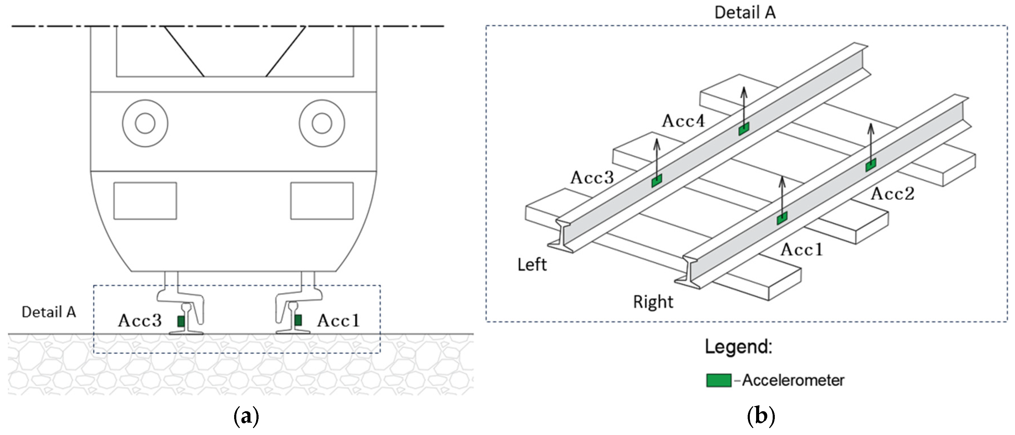
3.1. Wayside System Layout

A conceptual wayside monitoring system is defined to assess rail accelerations resulting from the passage of a train. In previous work [27], it was concluded that with a minimum number of two sensors (one on each rail), it was possible to detect out-of-roundness (OOR) defects in wheels. Therefore, four accelerometers were initially considered (two on each rail) for developing the polygonal wheel classification methodology in the present work. These accelerometers are installed on the rail at mid-span between two sleepers, where maximum bending deformations are obtained. The accelerometers are positioned precisely in the rail flange on the right side of the rail (Acc1 and Acc2) and the left side of the rail (Acc3 and Acc4), as depicted in Figure 2.

3.2. Vehicle-Track Dynamic Interaction

Train-track dynamic interaction is simulated using VSI software (Vehicle-Structure Interaction Analysis), whose validation and detailed description are provided in other publications by the authors [50,51]. In this model, the train is integrated with the track through a 3D wheel–rail contact model, wherein Hertzian theory is employed to compute the normal contact forces. Additionally, the USETAB routine is used to calculate the tangential forces arising from the rolling friction creep phenomenon.

This numerical tool is implemented in MATLAB^® [52] and imports the structural matrices from both the vehicle and track previously modeled in ANSYS^® [53]. The vehicle model is a Laagrss-type wagon developed and presented in detail in the work of Bragança et al. [54]. The track model can be found in [17,55] using beam elements to represent the rails and the sleepers, discrete mass points to simulate the ballast, and spring elements connecting all the components.

Wheel and track irregularities are previously geometrically characterized in MATLAB^® [52] and subsequently integrated into the constraint equations that couple the train to the track in the VSI software. By employing Lagrange multipliers, this tool connects wheel displacements with the track nodal displacements, incorporating track and wheel irregularities through a set of constraint equations. These equations are solved alongside equilibrium equations, forming a unified system that couples the two subsystems (see [50] for a full description of the coupling model).

A schematic representation of the numerical model is shown in Figure 3. The first wheel of the first wagon on the right side is considered a defective wheel (marked in green).

3.3. Wheel Irregularities

3.3.1. Characterization

New wheels in railway vehicles are not completely perfect and smooth, as they present irregularities along their surface. Polygonal wheels can be characterized by various geometric parameters, including the wavelength ($\mathsf{\Lambda }$), which varies based on the harmonic order ($\theta$) and the wheel radius ($R_w$). This relationship is defined by the following function:

$$\mathsf{\Lambda }=\frac{2\pi R_w}{\theta },\theta =\mathrm{1,2},3\dots ,n$$

(1)

The wheel irregularity level spectrum Lw (in dB re 1 μm) is defined by:

$$L_w=20{\mathrm{l}\mathrm{o}\mathrm{g}}_{10}\left(\frac{\widehat{\mathrm{w}}}{w_{ref}}\right)$$

(2)

where $\widehat{\mathrm{w}}$ is the root mean square value of the irregularity profile $w\left(x_w\right)$, evaluated for wavelengths corresponding to each OOR order, and $w_{ref}=1\mathsf{\mu }\mathrm{m}$.

To characterize the geometry of this type of imperfection, the average experimental measurements of four new wheels by Johansson et al. [5] are considered. The same procedure was adopted to characterize polygonal wheel defects, where the irregularity level spectrum Lw associated with each of the harmonics is based on experimental measurements [56,57,58]. Figure 4 depicts the level of irregularity related to each dominant harmonics. To cover a wide spectrum of harmonics, profiles with dominant harmonics between 6–8, measured by Cai et al. [56]; between 12–14, measured by Tao et al. [57]; and between 17–18, measured by Wu et al. [58], are considered. Additionally, the Figure also includes the wheel profile based on the experimental measurements of Johansson et al. [5] nominated new wheel in this study.

The polygonal wheel profile results from the superposition of all waves of harmonics and levels of irregularity associated with each harmonic. Then, different polygonal wheel profiles are generated based on the sum of sine functions (H = 30) as follows:

$$w\left(x_w\right)={\sum }_{\theta =1}^H{A}_{\theta }\sin \left(\frac{2\pi }{\mathsf{\Lambda }}{x}_w+{\mathsf{\psi }}_{\theta }\right)$$

(3)

where $x_w$ is the distance along wheel circumference and $A_{\theta }$ is the amplitude of the sine function for each $\mathsf{\Lambda },$ which is computed using the following function:

$$A_{\theta }=\sqrt{2}·{10}^{\frac{L_w}{20}}·w_{ref}$$

(4)

whereas $w_{ref}=1\mathsf{\mu }\mathrm{m}.$ The wheel irregularity level (Lw) values are selected based on the irregularity spectrums of Figure 4, for all scenarios: new wheels or polygonal wheels.

Considering different phase angles (${\mathsf{\psi }}_{\theta }$) in the sinusoidal functions uniformly and randomly distributed in the range from 0 to 2π, five cases are generated for each wheel defect amplitude based on each polygonal wheel irregularity spectrum.

3.3.2. Wheel Profiles

Two groups of defect amplitudes for each type of polygonal wheels are defined: group A1 (0.2–0.4 mm) and A2 (0.6–0.8 mm). Thus, a scale factor is applied to Equation (3) to generate the wheel polygonal profiles with different amplitudes. Figure 5 shows the three different types of profiles with dominant harmonic orders that are developed according to the irregularity profiles presented in Figure 4. In addition, in each of these profiles, two examples are plotted with defect amplitudes A1 and A2 and compared with the new wheel profile.

3.4. Track Irregularity Profiles

Based on European Standard EN 13848-2 [59], four different artificial irregularity profiles are used to generate vertical and lateral track irregularities for both rails. In this case, power spectral density (PSD) curves are developed [55] and then artificial irregularity profiles are generated in the vertical and transverse directions for wavelengths between 1 m and 75 m with a sampling discretization of 1 mm, covering the wavelength range intervals D1 and D2 defined by the European Standard EN 13848-2 [59]. Figure 6 shows an example of an irregular rail profile, which includes lateral misalignment and vertical unevenness on both rails.

3.5. Simulation Scenarios

Derived from various speeds, loading configurations, and rail irregularity profiles,

Table 1. Damaged and undamaged scenarios.

	Baseline Scenarios		Damaged Scenarios
	Perfect wheel	New wheel	Polygonal wheel
Vehicle	five freight wagons of the Laagrss type
Number of loading schemes	3	1 (full load)	1 (full load)
Unevenness profile	4	1	3
Speed range	40–120 km/h	80 km/h	80 km/h
Noise Ratio	5%	5%	5%
Location		1st wagon 3rd wagon 5th wagon	1st wagon
Harmonic orders ($\theta$)	-	-	H6-8 H12-14 H17-18
Amplitude ranges (W)	-	0.030–0.040 mm	A1 [0.2–0.4] mm A2 [0.6–0.8] mm
Total analyses	55	30	30

provides an overview of the simulations conducted for both undamaged and damaged scenarios.

The baseline scenarios comprise crossing speeds ranging from 40 to 120 km/h and four distinct rail irregularity profiles. The loading schemes used are empty, half-loaded, full-loaded. For simulations of the baseline scenarios, a combination of perfect wheels and new wheels (defined in Section 3.3) is used. The baseline scenarios consist of 55 simulations with perfect wheels and 30 simulations with new wheel profiles. The simulations with new wheel profiles are carried out at different locations, in the first, third, and fifth wagons. For the damaged scenarios, a total of 30 scenarios of polygonal wheels were generated with combinations of harmonic orders and defect amplitudes. For these simulations, a single defective wheel located on the first wagon on the right front wheel, and fully loaded wagons operating at a speed of 80 km/h are considered.

3.6. Track Dynamic Response

Acceleration signals are fixed at a sampling frequency of 10 kHz for all simulations. Subsequently, a Chebyshev type II digital low-pass filter with a cut-off frequency of 500 Hz is applied to filter the time series. Therefore, this high sampling frequency can increase the variance of the subsequently extracted damage features [60]. Furthermore, an artificial noise equivalent to 5% of the maximum acceleration of the initial signal is included in the numerical signal to provide a more realistic depiction of the measured rail response [51]. Figure 7 presents two acceleration time series plots, where the excitation promoted by the polygonal damage for all profiles is notorious, with a substantial increase in the vertical acceleration values when compared to a passage with new wheels. In addition, the influence of the amplitude of the polygonal damage on the measured responses is quite considerable: by comparing Figure 7a and 7b, it is visible that for an amplitude A1, the maximum response is approximately 40 m/s², while for an amplitude A2, the maximum response is around 100 m/s².

The acceleration responses are transformed to the frequency domain by applying an FFT algorithm to capture the excitation frequencies induced by each of the polygonal wheel profiles (Figure 8). The excitation frequency induced by the polygonal wheels can be given by the following expression:

$$f_{pol.}=\frac{v}{2\pi R_w}.n$$

(5)

where $v$ is the speed, $R_w$ the wheel radius, and $n$ is the number of harmonics. Based on Equation (5) and knowing that the adopted speed was always 80 km/h, it is possible to predict which dominant frequencies are excited for each harmonic profile (H6-8, H12-14 and H18-19). Assuming n is equal to the value of the order of the dominant harmonic in each of the profiles, a range of excitation frequencies of 50–65 Hz, 100–115 Hz, and 150–155 Hz are obtained using Equation (5), respectively. From the analysis of Figure 8, we can observe the frequency peaks for the H12-14 and H18-19 profiles around the expected values, while for the profile H6-8, a flat spectrum is obtained without showing any significant peak frequency. This can be explained by a smooth damage profile related to this harmonic group (Figure 4), which has a less evident harmonic peak than the other two profiles.

4. Automatic Classification of Polygonal Wheels

4.1. Feature Extraction

From the first phase of the methodology, the features are extracted based on applying the CWT and PCA models to the evaluated FFT responses. The results are evaluated for a set of four sensors (two on each side) located on the rail at mid-span between the sleepers. The main idea of feature extraction is to get a dimensionality reduction that identifies important relationships in the data.

For CWT features, the principal components are determined after extracting wavelet coefficients. Furthermore, four statistical parameters are derived from the scores, encompassing the root mean square (RMS), standard deviation, skewness, and kurtosis. For each sensor and every passage of the train, a total of 324 features are extracted. For PCA features, following the computation of the principal components, the same four statistical parameters are derived from the PCA scores. A total of 4 features are extracted for each sensor and passage.

For each sensor, the extracted features form a matrix of n × m, where n represents the number of train passages associated with the baseline or polygonal wheel scenarios, with a total of 115 simulations (mentioned in Table 1), and m represents the number of extracted features. Thus, for each method, the dimension of the matrix is as follows:

• Matrix X_PCA with 115 × 4, PCA features;
• Matrix X_CWT with 115 × 324, CWT features.

Figure 9 shows four features (two PCA statistical parameters and two wavelet coefficients) extracted by accelerometer 2. By analyzing the Figure, all features are already visible at this first step, leading to a tendency to distinguish between damaged and undamaged passages. The PCA features seem more sensitive to operational conditions, namely speed, than the CWT features showing more dispersed results in the baseline scenarios. Moreover, at this stage, a tendency is already noticeable in the PCA features to group the damage results according to the type of profile (dominant harmonics), while the CWT features seem to be more sensitive to the defect amplitude variations in each of the simulated profiles.

4.2. Data Fusion

Following feature normalization, a data fusion is performed to enhance the sensitivity of the features to abnormal cases.

To merge the features obtained through the PCA and CWT techniques, the Mahalanobis Distance (MD) is applied for each sensor as follows:

$$MD=\sqrt{\left(x_i-\overline{x}\right)·C^{-1}{·\left(x_i-\overline{x}\right)}^T}$$

(6)

in which $x_i$ is the matrix of extracted features, $\overline{x}$ is a mean vector of the features from the baseline simulation, and the inverse covariance matrix of the baseline simulation is defined by $C^{-1}$. In the first step, all features are merged (Figure 10a) and later, all sensors are merged (Figure 10b). In the first fusion step, a 115 × 1 vector is obtained for each of the four sensors and 115 train passages. Then, in the second fusion stage, a single 115 × 1 vector is obtained, in which the information from all four sensors is combined for each train passage. Figure 10, based on the PCA technique, shows that the second step of the merger considerably increases the damage sensitivity. This approach groups the polygonal wheel profiles according to the dominant harmonic.

On the other hand, as depicted in Figure 11, an approach using the CWT technique ensures a classification concerning the defect amplitude in each of the profiles. The first-order fusion is very sensitive to categorization by amplitude level; however, the second-order fusion promotes less dispersion in the results for the damage scenarios. The CWT model gains sensitivity for the categorization of the different wear amplitudes when all sensor information is merged. It is concluded that for a categorization by defect amplitude, the second fusion level will be adopted in this approach.

4.3. Feature Classification

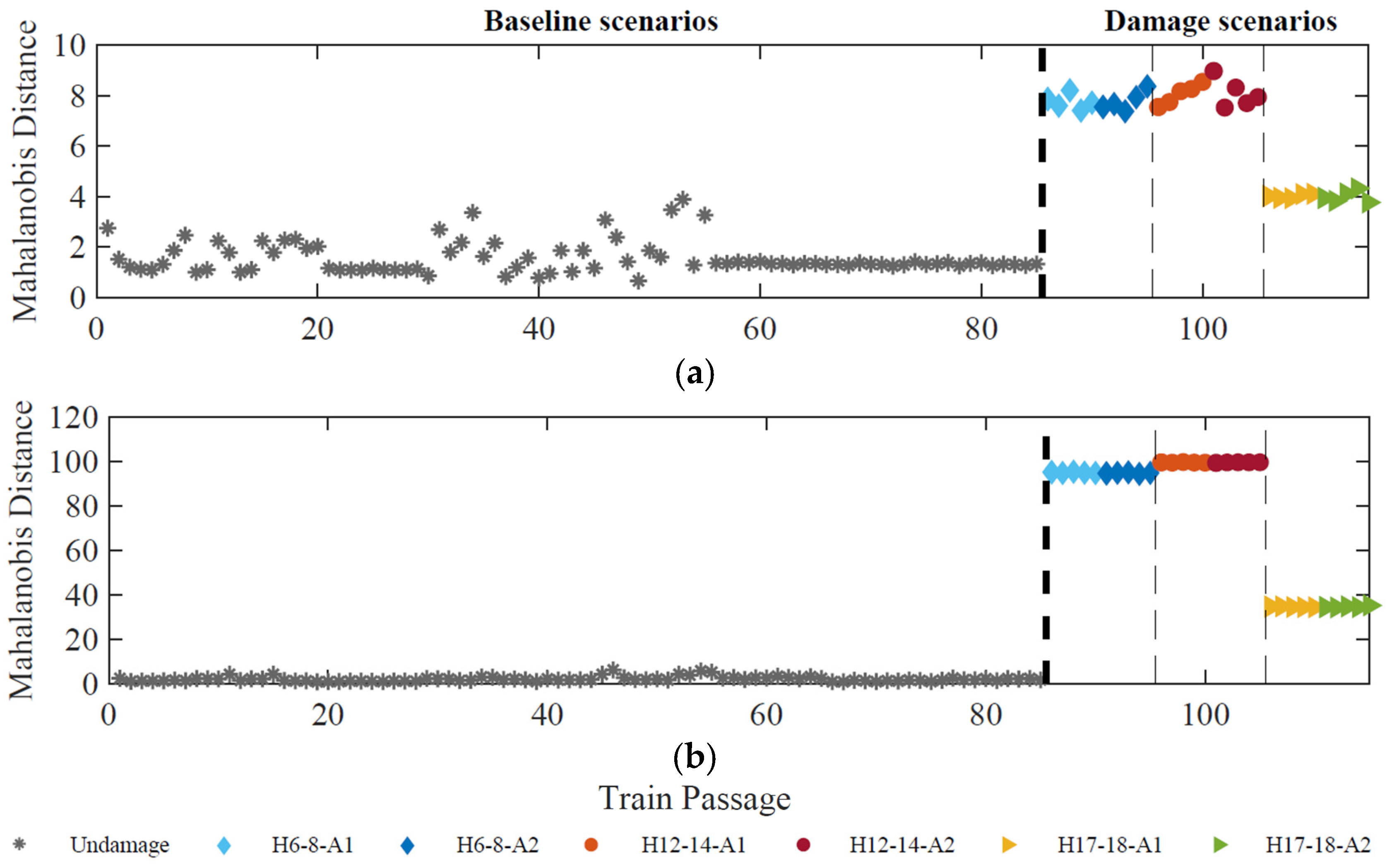
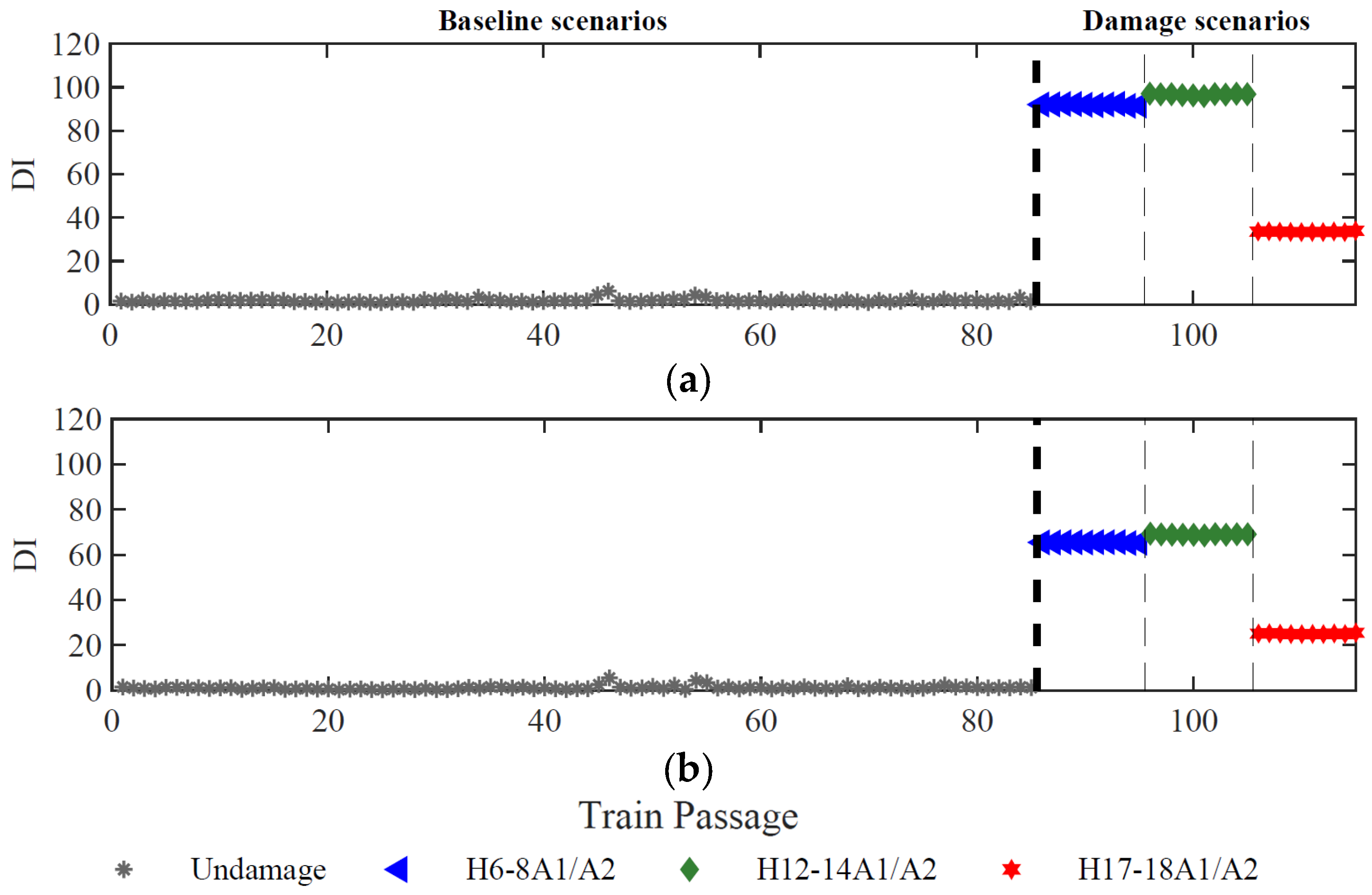
4.3.1. Harmonics-Based Classification

Based on the PCA features, the methodology classifies according to the dominant harmonics (Figure 12). A sensitivity analysis is performed to evaluate the optimized number of sensors used to classify polygonal wheels. The results using four and two accelerometers are plotted in Figure 12a,b, respectively. The DI amplitude decreases with the reduction in the number of sensors. However, in all sensor numbers, the methodology is shown to be very efficient, without any false classification. The maximum intra-cluster distance (ICD) observed for both sensor layouts, with four and two accelerometers, is 1.12 and 0.78, respectively.

4.3.2. Amplitude-Based Classification

Based on the CWT model, the methodology classifies according to the defect amplitude (Figure 13). The same as the PCA model, the clustering of the CWT features uses all sensor information, after the sensor fusion step. A sensitivity analysis is also performed to evaluate the optimized number of sensors used to classify polygonal wheels according to the defect amplitude. The results are evaluated using four sensors, with two on each side of the rail (Figure 13a), and two sensors, with one on each side of the rail (Figure 13b). The methodology proved very efficient, without any false classification and the DI remains unchanged regardless of the number of sensors. The maximum ICD for the two sensor layouts, four and two accelerometers, is 332.4 and 344.3, respectively.

5. Conclusions

This work proposes an automatic methodology based on machine learning that can accurately classify different types of polygonal damage in freight vehicle wheels. Two different feature extraction methods are performed, one consisting of the PCA method and the other based on the CWT model to transform acceleration signals into sensitive features for polygonal wheel classification.

The methodology proves to be highly effective in classifying polygonal wheels, with all tested scenarios correctly classified. The PCA features proved very effective for classifying harmonic-based polygonal wheels, with a stable damage index according to each dominant harmonic, resulting in no false classification. The results prove that the features are highly sensitive to the excitation frequencies caused by different orders of dominant harmonics since a considerable range was tested. The extracted features based on the CWT model are very sensitive to the defect amplitudes, regardless of the type of harmonic profile, classifying the two considered amplitude levels (A1 and A2) without any false classification. From an economic point of view, with only two accelerometers, the methodology can effectively classify in terms of dominant harmonic orders and defect amplitudes. By installing sensors on each side of the rail, the methodology can classify polygonal wheels regardless of the side of the defective wheel.

As future developments, the proposed methodology will be validated through experimental tests based on on-site measurements in which the polygonal wheels are previously characterized. To increase the robustness of the methodology, additional scenarios should be tested, considering multiple damages, different operating speeds, and vehicle types. Furthermore, upgrading the current methodology to localize polygonal wheels in multiple wagons of a freight train will also be considered.

References

1. Nielsen, J.C.O.; Johansson, A. Out-of-round railway wheels—A literature survey. Proc. Inst. Mech. Eng. Part F J. Rail Rapid Transit 2000, 214, 79–91. [Google Scholar] [CrossRef]
2. Barke, D.; Chiu, W.K. Structural Health Monitoring in the Railway Industry: A Review. Struct. Health Monit. 2005, 4, 81–93. [Google Scholar] [CrossRef]
3. Nielsen, J.C.O.; Lundén, R.; Johansson, A.; Vernersson, T. Train-Track Interaction and Mechanisms of Irregular Wear on Wheel and Rail Surfaces. Veh. Syst. Dyn. 2003, 40, 3–54. [Google Scholar] [CrossRef]
4. Chong, S.Y.; Shin, H. A review of health and operation monitoring technologies for trains. Smart Struct. Syst. 2010, 6, 1079–1105. [Google Scholar] [CrossRef]
5. Johansson, A.; Andersson, C. Out-of-round railway wheels—A study of wheel polygonalization through simulation of three-dimensional wheel-rail interaction and wear. Veh. Syst. Dyn. 2005, 43, 539–559. [Google Scholar] [CrossRef]
6. Peng, B. Mechanisms of Railway Wheel Polygonization. Ph.D. Thesis, University of Huddersfield, Huddersfield, UK, 2020. [Google Scholar]
7. Ni, Y.-Q.; Zhang, Q.-H. A Bayesian machine learning approach for online detection of railway wheel defects using track-side monitoring. Struct. Health Monit. 2021, 20, 1536–1550. [Google Scholar] [CrossRef]
8. Bogacz, R.; Frischmuth, K. On dynamic effects of wheel–rail interaction in the case of Polygonalisation. Mech. Syst. Signal Process. 2016, 79, 166–173. [Google Scholar] [CrossRef]
9. Nielsen, J. 8—Out-of-round railway wheels. In Wheel–Rail Interface Handbook; Lewis, R., Olofsson, U., Eds.; Woodhead Publishing: Sawston, UK, 2009; pp. 245–279. [Google Scholar]
10. Zhang, J.; Han, G.-x.; Xiao, X.-b.; Wang, R.-q.; Zhao, Y.; Jin, X.-s. Influence of wheel polygonal wear on interior noise of high-speed trains. J. Zhejiang Univ. Sci. A 2014, 15, 1002–1018. [Google Scholar] [CrossRef]
11. Wu, X.; Chi, M.; Wu, P. Influence of polygonal wear of railway wheels on the wheel set axle stress. Veh. Syst. Dyn. 2015, 53, 1535–1554. [Google Scholar] [CrossRef]
12. Wu, X.; Rakheja, S.; Qu, S.; Wu, P.; Zeng, J.; Ahmed, A.K.W. Dynamic responses of a high-speed railway car due to wheel polygonalisation. Veh. Syst. Dyn. 2018, 56, 1817–1837. [Google Scholar] [CrossRef]
13. Żurek, Z.; Bizon, K.; Bernd, R. Supplementary magnetic tests for railway wheel sets. Transp. Probl. 2008, 3/2008, 5–10. [Google Scholar]
14. Dwyer-Joyce, R.S.; Yao, C.; Lewis, R.; Brunskill, H. An ultrasonic sensor for monitoring wheel flange/rail gauge corner contact. Proc. Inst. Mech. Eng. Part F J. Rail Rapid Transit 2012, 227, 188–195. [Google Scholar] [CrossRef]
15. Li, C.; Luo, S.; Cole, C.; Spiryagin, M. An overview: Modern techniques for railway vehicle on-board health monitoring systems. Veh. Syst. Dyn. 2017, 55, 1045–1070. [Google Scholar] [CrossRef]
16. Sun, Q.; Chen, C.; Kemp, A.H.; Brooks, P. An on-board detection framework for polygon wear of railway wheel based on vibration acceleration of axle-box. Mech. Syst. Signal Process. 2021, 153, 107540. [Google Scholar] [CrossRef]
17. Mosleh, A.; Montenegro, P.A.; Alves Costa, P.; Calçada, R. An approach for wheel flat detection of railway train wheels using envelope spectrum analysis. Struct. Infrastruct. Eng. 2020, 17, 1710–1729. [Google Scholar] [CrossRef]
18. Lai, C.C.; Kam, J.C.P.; Leung, D.C.C.; Lee, T.K.Y.; Tam, A.Y.M.; Ho, S.L.; Tam, H.Y.; Liu, M.S.Y. Development of a Fiber-Optic Sensing System for Train Vibration and Train Weight Measurements in Hong Kong. J. Sens. 2012, 2012, 365165. [Google Scholar] [CrossRef]
19. Salzburger, H.-J.; Wang, L.; Gao, X. In-motion ultrasonic testing of the tread of high-speed railway wheels using the inspection system AUROPA III. Insight-Non-Destr. Test. Cond. Monit. 2009, 51, 370–372. [Google Scholar] [CrossRef]
20. Amini, A.; Entezami, M.; Huang, Z.; Rowshandel, H.; Papaelias, M. Wayside detection of faults in railway axle bearings using time spectral kurtosis analysis on high frequency acoustic emission signals. Adv. Mech. Eng. 2016, 8, 1687814016676000. [Google Scholar] [CrossRef]
21. Lagnebäck, R. Evaluation of Wayside Condition Monitoring Technologies for Condition-Based Maintenance of Railway Vehicles. Master’s Thesis, Luleå University of Technology, Luleå, Sweden, 2007; p. 119. [Google Scholar]
22. Kuźnar, M.; Lorenc, A. A Method of Predicting Wear and Damage of Pantograph Sliding Strips Based on Artificial Neural Networks. Materials 2022, 15, 98. [Google Scholar] [CrossRef] [PubMed]
23. Ye, Y.; Zhu, B.; Huang, P.; Peng, B. OORNet: A deep learning model for on-board condition monitoring and fault diagnosis of out-of-round wheels of high-speed trains. Measurement 2022, 199, 111268. [Google Scholar] [CrossRef]
24. Zhang, L.; Cheng, L.; Li, H.; Gao, J.; Yu, C.; Domel, R.; Yang, Y.; Tang, S.; Liu, W.K. Hierarchical deep-learning neural networks: Finite elements and beyond. Comput. Mech. 2021, 67, 207–230. [Google Scholar] [CrossRef]
25. Xu, Z.; Wang, H.; Xing, C.; Tao, T.; Mao, J.; Liu, Y. Physics guided wavelet convolutional neural network for wind-induced vibration modeling with application to structural dynamic reliability analysis. Eng. Struct. 2023, 297, 117027. [Google Scholar] [CrossRef]
26. Lieu, Q.X. A deep neural network-assisted metamodel for damage detection of trusses using incomplete time-series acceleration. Expert Syst. Appl. 2023, 233, 120967. [Google Scholar] [CrossRef]
27. Guedes, A.; Silva, R.; Ribeiro, D.; Vale, C.; Mosleh, A.; Montenegro, P.; Meixedo, A. Detection of Wheel Polygonization Based on Wayside Monitoring and Artificial Intelligence. Sensors 2023, 23, 2188. [Google Scholar] [CrossRef]
28. Meixedo, A.; Ribeiro, D.; Santos, J.; Calçada, R.; Todd, M.D. Real-Time Unsupervised Detection of Early Damage in Railway Bridges Using Traffic-Induced Responses. In Structural Health Monitoring Based on Data Science Techniques; Cury, A., Ribeiro, D., Ubertini, F., Todd, M.D., Eds.; Springer International Publishing: Cham, Germany, 2022; pp. 117–142. [Google Scholar]
29. Mohammadi, M.; Mosleh, A.; Vale, C.; Ribeiro, D.; Montenegro, P.; Meixedo, A. An Unsupervised Learning Approach for Wayside Train Wheel Flat Detection. Sensors 2023, 23, 1910. [Google Scholar] [CrossRef]
30. Wang, Q.; Xiao, Z.; Zhou, J.; Gong, D.; Wang, Z.; Zhang, Z.; Wang, T.; He, Y. A new DFT-based dynamic detection framework for polygonal wear state of railway wheel. Veh. Syst. Dyn. 2023, 61, 2051–2073. [Google Scholar] [CrossRef]
31. Song, Y.; Liang, L.; Du, Y.; Sun, B. Railway Polygonized Wheel Detection Based on Numerical Time-Frequency Analysis of Axle-Box Acceleration. Appl. Sci. 2020, 10, 1613. [Google Scholar] [CrossRef]
32. Chen, S.; Wang, K.; Zhou, Z.; Yang, Y.; Chen, Z. Quantitative detection of locomotive wheel polygonization under non-stationary conditions by adaptive chirp mode decomposition. Railw. Eng. Sci. 2022, 30, 129–147. [Google Scholar] [CrossRef]
33. Xie, B.; Chen, S.; Xu, M.; Dong, M.; Wang, K. Parameter Identification of Wheel Polygonization Based on Effective Signal Extraction and Inertial Principle. IEEE Sens. J. 2023, 23, 5061–5072. [Google Scholar] [CrossRef]
34. Ye, Y.; Wei, L.; Li, F.; Zeng, J.; Hecht, M. Multislice Time-Frequency image Entropy as a feature for railway wheel fault diagnosis. Measurement 2023, 216, 112862. [Google Scholar] [CrossRef]
35. Ye, Y.; Huang, C.; Zeng, J.; Zhou, Y.; Li, F. Shock detection of rotating machinery based on activated time-domain images and deep learning: An application to railway wheel flat detection. Mech. Syst. Signal Process. 2023, 186, 109856. [Google Scholar] [CrossRef]
36. Stratman, B.; Liu, Y.; Mahadevan, S. Structural Health Monitoring of Railroad Wheels Using Wheel Impact Load Detectors. J. Fail. Anal. Prev. 2007, 7, 218–225. [Google Scholar] [CrossRef]
37. Johansson, A.; Nielsen, J. Out-of-round railway wheels—Wheel-rail contact forces and track response derived from field tests and numerical simulations. Proc. Inst. Mech. Eng. Part F J. Rail Rapid Transit 2003, 217, 135–146. [Google Scholar] [CrossRef]
38. Zhou, C.; Gao, L.; Xiao, H.; Hou, B. Railway Wheel Flat Recognition and Precise Positioning Method Based on Multisensor Arrays. Appl. Sci. 2020, 10, 1297. [Google Scholar] [CrossRef]
39. Alemi, A.; Corman, F.; Pang, Y.; Lodewijks, G. Reconstruction of an informative railway wheel defect signal from wheel–rail contact signals measured by multiple wayside sensors. Proc. Inst. Mech. Eng. Part F J. Rail Rapid Transit 2018, 233, 49–62. [Google Scholar] [CrossRef]
40. Skarlatos, D.; Karakasis, K.; Trochidis, A. Railway wheel fault diagnosis using a fuzzy-logic method. Appl. Acoust. 2004, 65, 951–966. [Google Scholar] [CrossRef]
41. Belotti, V.; Crenna, F.; Michelini, R.C.; Rossi, G.B. Wheel-flat diagnostic tool via wavelet transform. Mech. Syst. Signal Process. 2006, 20, 1953–1966. [Google Scholar] [CrossRef]
42. Lourenço, A.; Ferraz, C.; Ribeiro, D.; Mosleh, A.; Montenegro, P.; Vale, C.; Meixedo, A.; Marreiros, G. Adaptive time series representation for out-of-round railway wheels fault diagnosis in wayside monitoring. Eng. Fail. Anal. 2023, 152, 107433. [Google Scholar] [CrossRef]
43. Wang, Y.W.; Ni, Y.Q.; Wang, X. Real-time defect detection of high-speed train wheels by using Bayesian forecasting and dynamic model. Mech. Syst. Signal Process. 2020, 139, 106654. [Google Scholar] [CrossRef]
44. Liu, X.-Z.; Ni, Y.-Q. Wheel tread defect detection for high-speed trains using FBG-based online monitoring techniques. Smart Struct. Syst. 2018, 21, 687–694. [Google Scholar]
45. Meixedo, A.; Ribeiro, D.; Santos, J.; Calçada, R.; Todd, M. 18—Structural health monitoring strategy for damage detection in railway bridges using traffic induced dynamic responses. In Rail Infrastructure Resilience; Calçada, R., Kaewunruen, S., Eds.; Woodhead Publishing: Sawston, UK, 2022; pp. 389–408. [Google Scholar]
46. Yan, A.-M.; Kerschen, G.; Boe, P.; Golinval, J.C. Structural damage diagnosis under varying environmental conditions—Part I: A linear analysis. Mech. Syst. Signal Process. 2005, 19, 847–864. [Google Scholar] [CrossRef]
47. Addison, P.S. Introduction to redundancy rules: The continuous wavelet transform comes of age. Philos. Trans. R. Soc. A 2018, 376, 20170258. [Google Scholar] [CrossRef]
48. Pan, Y.; Sun, Y.; Li, Z.; Gardoni, P. Machine learning approaches to estimate suspension parameters for performance degradation assessment using accurate dynamic simulations. Reliab. Eng. Syst. Saf. 2023, 230, 108950. [Google Scholar] [CrossRef]
49. Arthur, D.; Vassilvitskii, S. k-means++: The advantages of careful seeding. In Proceedings of the Eighteenth Annual ACM-SIAM Symposium on Discrete Algorithms, New Orleans, LA, USA, 7–9 January 2007; Society for Industrial and Applied Mathematics: New Orleans, LA, USA, 2007; pp. 1027–1035. [Google Scholar]
50. Montenegro, P.A.; Calçada, R. Wheel–rail contact model for railway vehicle–structure interaction applications: Development and validation. Railw. Eng. Sci. 2023, 31, 181–206. [Google Scholar] [CrossRef]
51. Mosleh, A.; Montenegro, P.A.; Costa, P.A.; Calçada, R. Railway Vehicle Wheel Flat Detection with Multiple Records Using Spectral Kurtosis Analysis. Appl. Sci. 2021, 11, 4002. [Google Scholar] [CrossRef]
52. MATLAB®, version R2018a; The MathWorks Inc.: Natick, MA, USA, 2018.
53. ANSYS®, ANSYS, Inc.: Canonsburg, PA, USA.
54. Bragança, C.; Neto, J.; Pinto, N.; Montenegro, P.A.; Ribeiro, D.; Carvalho, H.; Calçada, R. Calibration and validation of a freight wagon dynamic model in operating conditions based on limited experimental data. Veh. Syst. Dyn. 2022, 60, 3024–3050. [Google Scholar] [CrossRef]
55. Mosleh, A.; PCosta, A.; Calçada, R. A new strategy to estimate static loads for the dynamic weighing in motion of railway vehicles. Proc. Inst. Mech. Eng. Part F J. Rail Rapid Transit 2020, 234, 183–200. [Google Scholar] [CrossRef]
56. Cai, W.; Chi, M.; Tao, G.; Wu, X.; Wen, Z. Experimental and Numerical Investigation into Formation of Metro Wheel Polygonalization. Shock. Vib. 2019, 2019, 1538273. [Google Scholar] [CrossRef]
57. Tao, G.; Xie, C.; Wang, H.; Yang, X.; Ding, C.; Wen, Z. An investigation into the mechanism of high-order polygonal wear of metro train wheels and its mitigation measures. Veh. Syst. Dyn. 2021, 59, 1557–1572. [Google Scholar] [CrossRef]
58. Wu, X.; Rakheja, S.; Cai, W.; Chi, M.; Ahmed, A.K.W.; Qu, S. A study of formation of high order wheel polygonalization. Wear 2019, 424–425, 1–14. [Google Scholar] [CrossRef]
59. EN 13848-2; Railway Applications—Track—Track Geometry Quality—Part 2: Measuring Systems—Track Recording Vehicles. European Committee for Standardization: Brussels, Switzerland, 2006.
60. Casas, J.R.; Moughty, J.J. Bridge Damage Detection Based on Vibration Data: Past and New Developments. Front. Built Environ. 2017, 3, 4. [Google Scholar] [CrossRef]
Figure 1. Methodology for polygonal wheels classification.
Applsci 14 03650 g001
Figure 2. Wayside monitoring system layout: (a) front view, (b) 3D view.
Applsci 14 03650 g002
Figure 3. Graphical representation of the vehicle–track interaction model.
Applsci 14 03650 g003
Figure 4. Wheel irregularity amplitude spectra (Lw) and harmonic order (θ) for new and polygonal wheels.
Applsci 14 03650 g004
Figure 5. Examples of generated polygonal wheel profiles based on irregularity spectra: (a) H6-8, (b) H12-14, (c) H17-18.
Applsci 14 03650 g005aApplsci 14 03650 g005b
Figure 6. Example of a generated track irregularity profiles.
Applsci 14 03650 g006
Figure 7. Acceleration time series on position Acc2 for (a) healthy wheel and polygonal wheel with amplitude A1; (b) healthy wheel and polygonal wheel with amplitude A2.
Applsci 14 03650 g007
Figure 8. Frequency domain responses on position Acc2 for (a) healthy wheel and polygonal wheel with amplitude A1; (b) healthy wheel and polygonal wheel with amplitude A2.
Applsci 14 03650 g008
Figure 9. Feature extraction for accelerometer Acc2, (a) PCA–feature 1, (b) PCA–feature 3, (c) CWT–feature 173, (d) CWT–feature 193.
Applsci 14 03650 g009
Figure 10. Data fusion for PCA features: (a) 1st step fusion features for accelerometer Acc2 and (b) 2nd step fusion of all sensors.
Applsci 14 03650 g010
Figure 11. Data fusion for CWT features: (a) 1st step fusion features for accelerometer Acc2 and (b) 2nd step fusion of all sensors.
Applsci 14 03650 g011
Figure 12. Cluster analysis for harmonic-based classification using: (a) 4 sensors and (b) 2 sensors.
Applsci 14 03650 g012
Figure 13. Cluster analysis for amplitude-based classification using: (a) 4 sensors and (b) 2 sensors.
Applsci 14 03650 g013