


Monitoring Horizontal Displacements with Low-Cost GNSS Systems Using Relative Positioning: Performance Analysis


Department of Geomatics Engineering, Yıldız Technical University, 34220 Istanbul, Turkey
*
Author to whom correspondence should be addressed.
Appl. Sci. 2024, 14(9), 3634; https://0-doi-org.brum.beds.ac.uk/10.3390/app14093634
Submission received: 29 February 2024
/
Revised: 26 March 2024
/
Accepted: 28 March 2024
/
Published: 25 April 2024
(This article belongs to the Special Issue Identification and Measurement of Displacements and Deformations of Engineering Structures: 2nd Edition)
Abstract
:Monitoring horizontal displacements, such as landslides and tectonic movements, holds great importance and high-cost geodetic GNSS equipment stands as a crucial tool for the precise determination of these displacements. As the utilization of low-cost GNSS systems continues to rise, there is a burgeoning interest in evaluating their efficacy in measuring such displacements. This evaluation is particularly vital as it explores the potential of these systems as alternatives to high-cost geodetic GNSS systems in similar applications, thereby contributing to their widespread adoption. In this study, we delve into the assessment of the potential of the dual-frequency U-Blox Zed-F9P GNSS system in conjunction with a calibrated survey antenna (AS-ANT2BCAL) for determining horizontal displacements. To simulate real-world scenarios, the Zeiss BRT 006 basis-reduktionstachymeter was employed as a simulation device, enabling the creation of horizontal displacements across nine different magnitudes, ranging from 2 mm to 50 mm in increments of 2, 4, 6, 8, 10, 20, 30, 40, and 50 mm. The accuracies of these simulated displacements were tested through low-cost GNSS observations conducted over a 24 h period in open-sky conditions. Additionally, variations in observation intervals, including 3, 6, 8, and 12 h intervals, were investigated, alongside the utilization of the relative positioning method. Throughout the testing phase, GNSS data were processed using the GAMIT/GLOBK GNSS (v10.7) software, renowned for its accuracy and reliability in geodetic applications. The insightful findings gleaned from these extensive tests shed light on the system’s capabilities, revealing crucial information regarding its minimum detectable displacements. Specifically, the results indicate that the minimum detectable displacements with the 3-sigma rule stand at 22.8 mm, 11.7 mm, 8.7 mm, and 4.8 mm for 3 h, 6 h, 8 h, and 12 h GNSS observations, respectively. Such findings are instrumental in comprehending the system’s performance under varying conditions, thereby informing decision-making processes and facilitating the adoption of suitable GNSS solutions for horizontal displacement monitoring tasks.
1. Introduction
GNSS technology is extensively utilized in geodetic monitoring studies of tectonic movements [1,2,3], landslides [4,5,6,7,8], and a variety of natural events which require high accuracy observations. Another field where GNSS technology is heavily employed is in structural health monitoring studies [9,10,11,12]. GNSS measurement and processing methods exhibit variability in correspondence with evolving application domains. During high-precision applications, such as monitoring tectonic movements, static and long-term observations with the relative positioning method are generally used. Studies by [13,14,15] elucidate the use of long-term static GNSS measurements and relative positioning methods in monitoring tectonic movements. On the other hand, applications such as monitoring landslides or engineering structures can be applied with Real-Time Kinematic (RTK) or Precise Point Positioning (PPP) methods. The RT-PPP method [16], combines RTK and PPP methods for real-time landslide monitoring. The advantages of RT-PPP over RTK, particularly in overcoming limitations related to baseline length, are highlighted. Ref. [4] explained the monitoring of displacements caused by landslides using the network-RTK method. Ref. [17] tested the accuracy of the single base RTK GNSS method up to a 50 km baseline length. They found that single base RTK GNSS methods give similar results to the network RTK method up to 50 km. Ref. [18] investigated the potential of the GNSS PPP method for displacement monitoring. They used geodetic GNSS equipment and compared the PPP results with relative positioning results. The results showed that the PPP method, based on a 24 h observation period, can determine horizontal displacements up to 1.5 cm. Yigit et al. [19] investigated the use of PPP and PPP-AR methods in structural health monitoring studies. Topal et al. [20] explained the applicability of the PPP method in monitoring engineering structures through shake table tests. Ref. [21] conducted studies on bridge monitoring using the RTK method, determining its accuracy in monitoring bridges.
Above, the studies primarily focused on determining displacements geodetically using high-cost dual-frequency and geodetic multi-GNSS receivers and antennas. However, due to advancements in GNSS technology, low-cost GNSS receivers and antennas have emerged as viable alternatives to high-cost geodetic equipment, and these alternatives are now widely adopted. Initially, these receivers and antennas were introduced as single-frequency, and numerous studies have been conducted to assess the accuracy of single-frequency low-cost GNSS receivers and antennas up to the present day [22,23,24]. In recent years, there has been a shift towards dual-frequency and multi-GNSS low-cost receivers and antennas, replacing single-frequency systems. The significant advantage of low-cost GNSS receivers and antennas is their affordability, costing approximately 10 times less than geodetic counterparts. This cost advantage has not only increased the usage of such equipment in geodetic studies, such as monitoring tectonic movements, landslides, and engineering structures, but has also contributed to a more accurate displacement determination with the spatial resolution it offers.
Several studies have investigated the usability and performance of low-cost GNSS equipment in geodetic monitoring and displacement determination. [25] conducted tests using the U-blox ZED-F9P receiver, low-cost U-blox ANN-MB-00 patch antenna, and geodetic Leica AS10 antenna to research the accuracy of low-cost GNSS receivers with the network RTK method. Although similar results to geodetic receivers were obtained with the low-cost U-blox ZED-F9P receiver, it was noted that satisfactory results were achieved only in clear sky conditions when the multipath effect was minimal. Ref. [26] aimed to test the accuracy of low-cost GNSS equipment for geodetic monitoring. The U-blox ZED-F9P receiver and ANN-MB-00 patch antenna were used, and the collected data were processed with RTKLIB software (demo5_b33b). The study concluded that displacements above 10 mm could be determined with low-cost equipment on short baselines, but accuracy was often insufficient. In the study by [27], the performance of low-cost GNSS equipment in determining horizontal displacements was examined using two different antenna types (low-cost patch and survey) and the PPP method. The results indicated that, with the survey antenna and PPP method, displacements of 20 mm within 3 h could be determined with an RMSE of 6 mm. It was also noted that the low-cost patch antenna was highly sensitive to multipath effects, and with 6 h of measurements, displacements of 30 mm could be determined with an RMSE of 15 mm.
Ref. [28] conducted a study testing the performance of low-cost GNSS receivers in monitoring dynamic movements. In the study, the U-blox M8T receiver and patch antennas were utilized, and it was noted that low-cost GNSS receivers could determine the modal frequencies of bridges within the range of 0.362 Hz and 1.680 Hz. Ref. [29] investigated the accuracy of low-cost GNSS receivers in position determination using the RTK method applied in geodesy. The study reported accuracy values of ±5.5 mm for the horizontal position and ±11 mm for the vertical position. In the study by [30] low-cost GNSS receivers were employed to monitor displacements. The U-blox Neo-7P, a single-frequency and low-cost GNSS receiver, was used in the study. It was mentioned that on short baselines, displacements exceeding 15 mm in the horizontal direction could be determined using single-frequency and low-cost GNSS receivers. In the study conducted by [31], the performance of low-cost GNSS receivers and antennas was tested in urban areas, and the positioning accuracy of the RTK method was reported to be between 10 and 30 mm in the open-sky and urban areas. In [32], the performance of the low-cost GNSS system in positioning using the PPP-RTK method was tested. The results demonstrated that the u-blox ZED-F9P GNSS module could achieve centimeter-level positioning accuracy.
The objective of this study is to investigate the accuracy of determining horizontal displacements using low-cost GNSS receivers and antennas through the relative positioning method. To achieve this goal, displacements of different magnitudes were generated using the simulation equipment described in the following section. The data collected for determining displacements based on the measurement time with the low-cost GNSS receiver and antenna were processed using the GAMIT/GLOBK (v10.7) GNSS software [33]. Unlike previous studies, this research specifically explores the accuracy of determining horizontal displacements with low-cost GNSS equipment using the relative positioning method. Additionally, this study aims to identify the range of detectable displacements using GNSS relative positioning and to assess the impact of measurement time. Thus, the aim is to determine whether low-cost GNSS systems can serve as alternatives to geodetic GNSS systems in engineering measurements such as monitoring landslides and tectonic movements, where high accuracy is required. During the processing stage, IGS points were specifically chosen as reference points, similar to the approach used in studies monitoring tectonic movements. This was aimed at determining the performance of low-cost systems especially in monitoring tectonic movements.
This study consists of three main sections prepared for this purpose: Materials and Methods, Results and Discussion, and Conclusions. In the Section 2, the GNSS equipment used in this study, the test environment, and the conducted test procedures are described. The Section 3 examines the displacement values and their accuracies obtained through the processing of GNSS data. Finally, the Section 4 interprets the displacement determination accuracy using low-cost GNSS systems.
2. Materials and Methods
In the first quarter of 2019, a new generation of GNSS receivers entered the market, offering approximately 10 times lower costs compared to geodetic GNSS receivers and antennas. These new devices are multi-frequency (L1 and L2) and multi-system (supporting GPS, GLONASS, Galileo, and BeiDou) GNSS receivers. In this study, the u-Blox ZED-F9P low-cost GNSS receiver and AS-ANT2BCAL antenna from ArduSimple were employed. The technical features of the receiver and antenna are listed in Table 1 and Table 2, respectively, and Figure 1 displays the U-Blox GNSS receiver and antenna provided by Ardusimple. The calibration parameters of AS-ANT2BCAL antenna are published by the National Geodetic Survey (NGS) [34].
The data collection with the Ublox GNSS receiver was conducted using the u-center software (v22.02) developed by Ublox. The receiver was connected to the laptop, where the USB port was used for power supply as well as for data storage. The u-center software was installed on a laptop computer, which remained connected to the GNSS receiver throughout this study. GNSS data are collected in UBX format using the GNSS receivers. The GNSS data in UBX format can be converted to Rinex format using RTKCONV, a module of the RTKLIB software (2.4.2) [35]. Throughout this study, raw GNSS data in UBX format was converted to Rinex format using the RTKCONV software (2.4.2), resulting in 24 h data files.
In the scope of this study, test measurements were conducted on the rooftop of the Faculty of Civil Engineering at Yıldız Technical University, specifically at the pillar named UZEL (Figure 2). At the UZEL GNSS station, there is an electrical panel that can be powered from the city power grid, and at the same time, with the help of solar panels, batteries, and other equipment, the system can operate uninterrupted with its own generated energy when it cannot receive electricity from the city power grid.
The AS-ANT2BCAL low-cost GNSS antenna was mounted on the Zeiss BRT 006 basis-reduktionstachymeter, and GNSS measurements were carried out over a period of 10 days (Figure 3).
The Zeiss BRT 006 basis-reduktionstachymeter allows for the measurement of horizontal directions, zenith distances, and lengths, as illustrated in Figure 4. Notably, it features optical distance measurement capabilities. The parallactic triangle, characterized by a fixed parallactic angle and a variable base at the station point, is rectangular. The prism, ensuring a constant angle, moves along the metal guide through a division. In the eyepiece, observers see a double image of the target point, one direct and the other provided by the moving prism. The prism is adjusted until the two images coincide. The position of the prism is read from the division, and, when converted into the appropriate unit, directly represents the horizontal distance to the point being measured. The precision of distance measurements is 0.06% or 0.03 mm per 5 cm.
To assess the displacement determination accuracy of the low-cost GNSS receiver, the GNSS antenna mounted on the Zeiss BRT 006 basis-reduktionstachymeter was sequentially moved by increments of 2, 4, 6, 8, 10, 20, 30, 40, and 50mm. Following each movement, GNSS data were collected continuously for a period of 24 h. This process was repeated over 10 days, constituting the test measurements throughout this study. The 24 h data obtained from the measurements were then divided into 3, 6, 8, and 12 h groups to analyze the impact of measurement duration on displacement determination accuracy. The TEQC software (2019 release) [36] was utilized to divide the 24 h data into 3, 6, 8, and 12 h segments. During the measurements, a data recording interval of 30 s was applied, and the measurements were conducted in an open-sky condition with a low multipath environment. The measurement schedule applied for various displacement magnitudes is given in Table 3. The time intervals of the 3, 6, 8, and 12 h data obtained by dividing the 24 h GNSS data are given in Table 4.
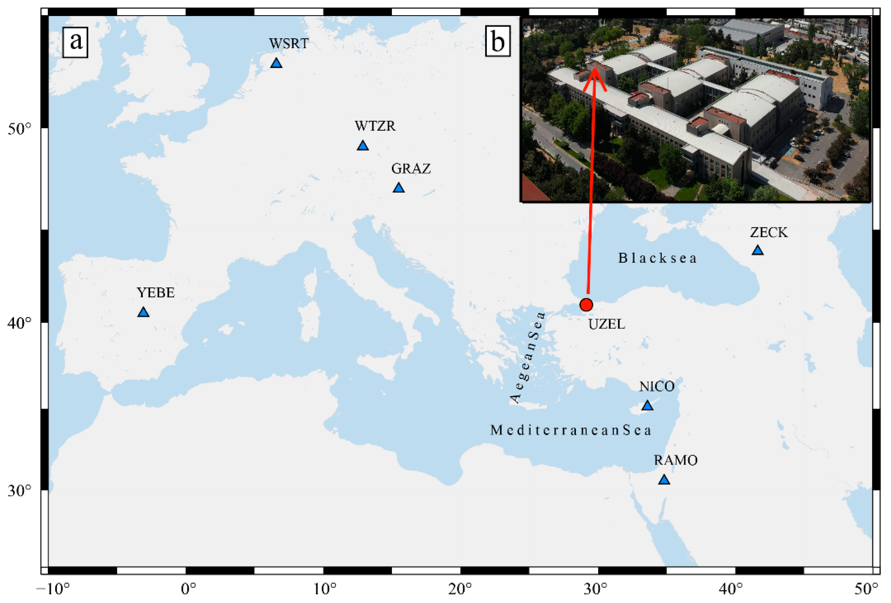
The GNSS data for the time intervals given in Table 4 were processed using the GAMIT/GLOBK software (v10.7). The data were analyzed in GAMIT software at first to estimate UZEL site coordinates with loose a priori constraints. To link our station to the global network, the IGS stations, shown in Figure 5 with blue triangles, were used in the analysis. NICO, RAMO, ZECK, GRAZ, WTZR, WSRT, and YEBE IGS stations were used for processing the GNSS data at UZEL station because of the data availability and stability of these stations. In the GLOBK (Global Kalman filter) stage, the output from GAMIT, as loosely constrained coordinate estimations, was used to estimate the daily coordinates. After obtaining precise coordinates, the differences between estimated coordinate values were compared with displacement values generated using the Zeiss BRT 006 basis-reduktionstachymeter.
Deformation of a point is defined as statistically significant displacement of the point between two epochs. The horizontal position of a point is Pt (nt, et) at time (t) and Pt+Δt (nt+Δt, et+Δt) at time (t + Δt). Displacement is determined by calculating the difference between the estimated coordinates at time (t) and time (t + Δt):
Horizontal displacement of a point P between time (t) and (t + Δt) is calculated as follows:
The errors were determined by subtracting each estimated horizontal displacement from the real displacement values for all the 3 h, 6 h, 8 h, 12 h, and 24 h observation times.
where d is the real displacement value, di is the estimated value, and εi is the error for the session i. The Root Mean Square Error is determined by Equation (4).
The values of di in Equation (2) were computed after processing the data with the GAMIT/GLOBK software. The value of d given in Equation (3) represents the known displacement values from Table 3, while di indicates the displacement values calculated using Equation (2) after the GAMIT/GLOBK processing. Since the displacement accuracy produced by the Zeiss BRT 006 basis-reduktionstachymeter is given as 0.06% or 0.03 mm per 5 cm, the artificially generated displacement values were considered as known values in this study. The differences between these known displacement values and the displacement values obtained from GNSS data are used as error values.
Calculations given above were performed based on the coordinate values determined from observations collected over a 24 h period. Additionally, processes were conducted to obtain coordinates from observations of 3, 6, 8, and 12 h durations derived from the same dataset. Since there was only a single observation for the 24 h period for each increment of 2, 4, 6, 8, 10, 20, 30, 40, and 50 mm, a RMSE could not be calculated for these datasets. However, RMSEs were computed for all other observations derived from the division of the 24 h data, and these values are subsequently shared in the Section 3.
3. Results and Discussion
Firstly, the differences in UZEL site daily coordinates obtained from data collected for 24 h using the dual-frequency U-Blox Zed-F9P GNSS system were divided into different durations and compared with the displacement values generated using the Zeiss BRT 006 basis-reduktionstachymeter. The error is defined by the difference between the observed displacements and the actual displacements. In this study, observed displacement refers to the displacement value obtained by processing and analyzing the GNSS observations while actual displacement refers to the displacement artificially generated using the Zeiss BRT 006 basis-redu-tionstachymeter.
Figure 6 illustrates the errors for the 3, 6, 8, and 12 h observation analysis results calculated by Equation (3) for each displacement value. When examining Figure 6, it is seen that displacement values of up to 20 mm cannot be accurately determined within the 3 h measurement period. For example, it is observed that when attempting to determine a displacement of 2 mm with 3 h measurements, a 12 mm error is obtained. Similarly, an attempt to ascertain a displacement of 4 mm through 3 h measurements results in a 15 mm error, and despite aiming to determine a displacement of 10 mm a discrepancy of 18 mm error is observed with the 3 h measurements. Based on similar results obtained for displacements up to 20 mm, it is apparent that 3 h measurements are insufficient for accurately determining displacement values of such magnitudes even with the relative positioning.
Figure 6 also shows that a duration time of more than 3 h gives less errors. It makes sense for longer duration measurements to be closer to the true values. Moreover, especially with measurements lasting 6 h or longer, significant results are obtained for all displacement values, and the error values significantly decrease. Furthermore, in Figure 6, it can be observed that as the displacement increases, the error amounts decrease.
Table 5 displays the Root Mean Square Error (RMSE) values, calculated with Equation (4), for the 3, 6, 8, and 12 h observation periods. Table 5 indicates that there is an improvement in RMSE values after the 6 h observation period for all displacements. It is observed that the RMSE values obtained with a 12 h observation period are the smallest.
When examining the RMSE values for the 3 h measurements, it is observed that insignificant results are obtained for displacement values smaller than 20mm. For instance, it is observed that for 3 h measurements, a 2 mm displacement can be determined with a 5.9 mm RMSE, a 4mm displacement with a 7.4 mm RMSE, and an 8 mm displacement with a 9.7 mm RMSE. Similarly, for the 6 h measurements, it is observed that results are insignificant for displacement values smaller than 4 mm. For instance, for 6 h measurements, a 2 mm displacement can be determined with a 2.1 mm RMSE. After 8 h, it is seen that the results are significant for all displacement values. This indicates that at least an 8 h measurement period is necessary to achieve significant results in displacement determination studies using low-cost GNSS systems with relative positioning.
To determine the minimum detectable displacement value based on the observation period, mean RMSE values of estimated displacements were calculated for datasets of the same length. The results are given in Table 6.
The 3-sigma method was employed to determine the minimum detectable displacement value using the RMSE values from Table 6. As shown in Table 6, the minimum detectable displacement values are 22.8 mm, 11.7 mm, 8.7 mm, and 4.8 mm for observation periods of 3 h, 6 h, 8 h, and 12 h, respectively. Ref. [18] reported minimum detectable displacements for relative positioning as 23.4 mm, 13.5 mm, 9.0 mm, and 8.4 mm for observation periods of 3 h, 6 h, 12 h, and 24 h, respectively, using geodetic-grade GNSS equipment. Ref. [27] reported that 20 mm displacement can be determined with 6 mm RMSE using the PPP approach based on a 3 h observation period by using low-cost GNSS equipment. Remarkably, similar results were obtained in this study despite the use of low-cost GNSS equipment, demonstrating comparable performance to geodetic GNSS equipment.
4. Conclusions
This study investigated the performance of low-cost GNSS equipment in determining horizontal displacements through the relative positioning method. Errors and RMSE values were assessed based on tests with varying observation times and displacement values. Analysis of RMSE values revealed significant improvements in accuracy, particularly after the 8 h observation period. This suggests that an observation period of at least 8 h is necessary to accurately determine displacement values with low-cost GNSS equipment through relative positioning. It can be said that an 8 h measurement period is necessary to attain high-precision results with low-cost GNSS systems, akin to high-cost geodetic GNSS systems, particularly in studies such as monitoring tectonic movements and landslides, where high accuracy is imperative.
However, this study identified the smallest displacement values that can be reliably determined with low-cost GNSS equipment as 22.8 mm, 11.7 mm, 8.7 mm, and 4.8 mm for observation periods of 3 h, 6 h, 8 h, and 12 h, respectively. These values closely align with a study conducted by [18] using geodetic GNSS equipment and [27] using PPP method and low-cost GNSS equipment. The consistency of the results suggests that low-cost GNSS equipment can achieve displacement values with a level of accuracy similar to that of geodetic instruments. These results indicate that low-cost GNSS systems can be used as alternatives to geodetic GNSS systems after 8 h of observation, particularly in engineering measurements where determining horizontal displacements is crucial, such as monitoring landslides, tectonic movements, and deformations in structures. The lower cost of these systems opens the possibility of monitoring larger areas with more GNSS equipment, indirectly enhancing the security of these regions. Thanks to their low costs, these systems can be set up as permanent and continuous GNSS stations, enabling the continuous monitoring of tectonic movements, landslides, and engineering structures. This, in turn, facilitates the timely detection of potential deformations.
It should be noted that these results are conducted in this study for displacement values. No velocity estimation has been performed in this study. The determination of annual velocity is crucial for tectonic studies, and future research may explore the possibility of velocity calculation for tectonic purposes using low-cost systems. Additionally, this study can be conducted using different GNSS processing software other than GAMIT/GLOBK. However, since the focus of this study was on displacement determination accuracy rather than positioning accuracy, it is believed that the results would not significantly change.
Author Contributions
Methodology, B.A.; Formal analysis, S.Ö.; Data curation, B.A.; Writing—original draft, B.A.; Writing—review & editing, S.Ö.; Visualization, S.Ö. All authors have read and agreed to the published version of the manuscript.
Funding
This research received no external funding.
Institutional Review Board Statement
Not applicable.
Informed Consent Statement
Not applicable.
Data Availability Statement
The original contributions presented in the study are included in the article, further inquiries can be directed to the corresponding authors.
Conflicts of Interest
The authors declare no conflicts of interest.
References
- Cakir, Z.; Dogan, U.; Akoğlu, A.M.; Ergintav, S.; Özarpacı, S.; Özdemir, A.; Nozadkhalil, T.; Çakır, N.; Zabcı, C.; Erkoç, M.H.; et al. Arrest of the Mw 6.8 January 24, 2020 Elaziğ (Turkey) earthquake by shallow fault creep. Earth Planet. Sci. Lett. 2023, 608, 118085. [Google Scholar] [CrossRef]
- Özkan, A.; Solak, H.İ.; Tiryakioğlu, İ.; Şentürk, M.D.; Aktuğ, B.; Gezgin, C.; Poyraz, F.; Duman, H.; Masson, F.; Uslular, G.; et al. Characterization of the co-seismic pattern and slip distribution of the February 06, 2023, Kahramanmaraş (Turkey) earthquakes (Mw 7.7 and Mw 7.6) with a dense GNSS network. Tectonophysics 2023, 866, 230041. [Google Scholar] [CrossRef]
- Vardic, K.; Clarge, P.J.; Whitehouse, P.L. A GNSS velocity field for crustal deformation studies: The influence of glacial isostatic adjustment on plate motion models. Geophys. J. Int. 2022, 231, 426–458. [Google Scholar] [CrossRef]
- Shu, B.; He, Y.; Wang, L.; Zhang, Q.; Li, X.; Qu, X.; Huang, G.; Qu, W. Real-time high-precision landslide displacement monitoring based on a GNSS CORS network. Measurement 2023, 217, 113056. [Google Scholar] [CrossRef]
- Wang, P.; Liu, H.; Nie, G.; Yang, Z.; Wu, J.; Qian, C.; Shu, B. Performance evaluation of a real-time high-precision landslide displacement detection algorithm based on GNSS virtual reference station technology. Measurement 2022, 199, 111457. [Google Scholar] [CrossRef]
- Segina, E.; Peternel, T.; Urbancic, T.; Realini, E.; Zupan, M.; Jez, J.; Caldera, S.; Gatti, A.; Tagliaferro, G.; Consoli, A.; et al. Monitoring Surface Displacement of a Deep-Seated Landslide by a Low-Cost and near Real-Time GNSS System. Remote Sens. 2020, 12, 3375. [Google Scholar] [CrossRef]
- Bellone, T.; Dabove, P.; Manzino, A.M.; Taglioretti, C. Real-time monitoring for fast deformations using GNSS low-cost receivers, Geomatics. Nat. Hazards Risk 2016, 7, 458–470. [Google Scholar] [CrossRef]
- Hamza, V.; Stopar, B.; Sterle, O.; Pavlovcic, P. A Cost-Effective GNSS Solution for Continuous Monitoring of Landslides. Remote Sens. 2023, 15, 2287. [Google Scholar] [CrossRef]
- Xi, R.; He, Q.; Meng, X. Bridge monitoring using multi-GNSS observations with high cutoff elevations: A case study. Measurement 2021, 168, 108303. [Google Scholar] [CrossRef]
- Paziewski, J.; Stepniak, K.; Sieradzki, R.; Yigit, C.O. Dynamic displacement monitoring by integrating high-rate GNSS and accelerometer: On the possibility of downsampling GNSS data at reference stations. GPS Solut. 2023, 27, 157. [Google Scholar] [CrossRef]
- Bezcioglu, M.; Yigit, C.O.; Mazzoni, A.; Fortunato, M.; Dindar, A.A.; Karadeniz, B. High-rate (20Hz) single-frequency GPS/GALILEO variometric approach for real-time structural health monitoring and rapid risk assessment. Adv. Space Res. 2022, 70, 1388–1405. [Google Scholar] [CrossRef]
- Caldera, S.; Barindelli, S.; Sanso, F.; Pardi, L. Monitoring of Structures and Infrastructures by Low-Cost GNSS Receivers. Appl. Sci. 2022, 12, 12468. [Google Scholar] [CrossRef]
- Konca, A.O.; Karabulut, H.; Güvercin, S.E.; Eskiköy, F.; Özarpacı, S.; Özdemir, A.; Floyd, M.; Doğan, U. From Interseismic Deformation with Near-Repeating Earthquakes to Co-Seismic Rupture: A Unified View of the 2020 Mw6.8 Sivrice (Elazığ) Eastern Turkey Earthquake. J. Geophys. Res. Solid Earth 2021, 126, e2021JB021830. [Google Scholar] [CrossRef]
- Gezgin, C.; Ekercin, S.; Tiryakioğlu, İ.; Aktuğ, B.; Erdoğan, H.; Gürbüz, E.; Orhan, O.; Bilgilioğlu, S.S.; Torun, A.T.; Gündüz, H.İ.; et al. Determination of Recent Tectonic Deformations Along the Tuz Gölü Fault Zone in Central Anatolia (Turkey) with Gnss Observations. Turkish J. Earth Sci. 2022, 31, 20–33. [Google Scholar]
- Abe, D.; Yoshioka, S. Spatiotemporal distributions of interplate coupling in Tohoku, northeast Japan, for 14 years prior to the 2011 Tohoku-oki earthquake inverted from GNSS data. Tectonophysics 2022, 838, 229479. [Google Scholar] [CrossRef]
- Hung, G.; Du, S.; Wang, D. GNSS techniques for real-time monitoring of landslides: A review. Satell. Navig. 2023, 4, 5. [Google Scholar] [CrossRef]
- Aykut, N.O.; Gülal, E.; Akpınar, B. Performance of Single Base RTK GNSS Method versus Network RTK. Earth Sci. Res. J. 2015, 19, 135–139. [Google Scholar] [CrossRef]
- Yigit, C.O.; Coskun, M.Z.; Yavasoglu, H.; Arslan, A.; Kalkan, Y. The potential of GPS Precise Point Positioning method for point displacement monitoring: A case study. Measurement 2016, 91, 398–404. [Google Scholar] [CrossRef]
- Yigit, C.O.; El-Mowafy, A.; Dindar, A.A.; Bezcioglu, M.; Tiyakioglu, I. Investigating Performance of High-Rate GNSS-PPP and PPP-AR for Structural Health Monitoring: Dynamic Tests on Shake Table. J. Surv. Eng. 2020, 147, 05020011. [Google Scholar] [CrossRef]
- Topal, G.; Akpinar, B. High rate GNSS kinematic PPP method performance for monitoring the engineering structures: Shake table tests under different satellite configurations. Measurement 2022, 189, 110451. [Google Scholar] [CrossRef]
- Xi, R.; Jiang, W.; Meng, X.; Chen, H.; Chen, Q. Bridge monitoring using BDS-RTK and GPS-RTK techniques. Measurement 2018, 120, 128–139. [Google Scholar] [CrossRef]
- Zuliani, D.; Tunini, L.; Traglia, F.D.; Chersich, M.; Curone, D. Cost-Effective, Single-Frequency GPS Network as a Tool for Landslide Monitoring. Sensors 2022, 22, 3526. [Google Scholar] [CrossRef]
- Qiu, D.; Wang, L.; Luo, D.; Huang, H.; Ye, Q.; Zhang, Y. Landslide monitoring analysis of single-frequency BDS/GPS combined positioning with constraints on deformation characteristics. Surv. Rev. 2019, 51, 364–372. [Google Scholar] [CrossRef]
- Squarzoni, C.; Delacourt, C.; Allemand, P. Differential single-frequency GPS monitoring of the La Valette landslide (French Alps). Eng. Geol. 2005, 79, 215–229. [Google Scholar] [CrossRef]
- Janos, D.; Kuras, P. Evaluation of Low-Cost GNSS Receiver under Demanding Conditions in RTK Network Mode. Sensors 2021, 21, 552. [Google Scholar] [CrossRef]
- Hamza, V.; Stopar, B.; Ambrozic, T.; Turk, G.; Sterle, O. Testing Multi-Frequency Low-Cost GNSS Receivers for Geodetic Monitoring Purposes. Sensors 2020, 20, 4375. [Google Scholar] [CrossRef]
- Topal, O.G.; Karabulut, M.F.; Aykut, N.O.; Akpınar, B. Performance of low-cost GNSS equipment in monitoring of horizontal displacements. Surv. Rev. 2023, 55, 536–545. [Google Scholar] [CrossRef]
- Xue, C.; Psimoulis, P.A.; Meng, X. Feasibility analysis of the performance of low-cost GNSS receivers in monitoring dynamic motion. Measurement 2022, 202, 111819. [Google Scholar] [CrossRef]
- Carretero-Garrido, M.S.; Lacy-Perez de los Cobos, M.C.; Borque-Arancon, M.J.; Ruiz-Armenteros, A.M.; Moreno-Guerrero, R.; Gil-Cruz, A.J. Low-cost GNSS receiver in RTK positioning under the standard ISO-17123-8: A feasible option in geomatics. Measurement 2019, 137, 168–178. [Google Scholar] [CrossRef]
- Biagi, L.; Grec, C.F.; Negretti, M. Low-Cost GNSS Receivers for Local Monitoring: Experimental Simulation, and Analysis of Displacements. Sensors 2016, 16, 2140. [Google Scholar] [CrossRef]
- Hamza, V.; Stopar, B.; Sterle, O.; Pavlovcic-Preseren, P. Low-Cost Dual-Frequency GNSS Receivers and Antennas for Surveying in Urban Areas. Sensors 2023, 23, 2861. [Google Scholar] [CrossRef]
- Robustelli, U.; Cutugno, M.; Publiano, G. Low-Cost GNSS and PPP-RTK: Investigating the Capabilities of the u-blox ZED-F9P Module. Sensors 2023, 23, 6074. [Google Scholar] [CrossRef]
- Herring, T.A.; King, R.W.; McClusky, S.C. Introduction to GAMIT/GLOBK; Release 10.35; Massachussetts Institute of Technology: Cambridge, MA, USA, 2009. [Google Scholar]
- National Geodetic Survey Antenna Calibration. Available online: https://geodesy.noaa.gov/ANTCAL/ (accessed on 26 March 2024).
- Takasu, T.; Yasuda, A. Development of the low-cost RTK-GPS receiver with an open-source program package RTKLIB. In Proceedings of the International Symposium on GPS/GNSS, Jeju, Republic of Korea, 4–6 November 2009. [Google Scholar]
- Estey, L.H.; Meertens, C.M. TEQC: The multi-purpose toolkit for GPS/GLONASS data. GPS Solut. 1999, 3, 42–49. [Google Scholar] [CrossRef]
Figure 1.
Low-cost GNSS receiver (U-Blox ZED-F9P and AS-ANT2BCAL antenna).

Figure 2.
UZEL test station.

Figure 3.
Experimental setup.

Figure 4.
Zeiss BRT 006 basis-reduktionstachymeter.

Figure 5.
(a) Blue triangles illustrate IGS stations used for GAMIT/GLOBK processing, and the red circle shows the location of the UZEL test site (b) Yıldız Technical University Civil Engineering Faculty and the UZEL test site on the roof of the faculty.
Figure 5.
(a) Blue triangles illustrate IGS stations used for GAMIT/GLOBK processing, and the red circle shows the location of the UZEL test site (b) Yıldız Technical University Civil Engineering Faculty and the UZEL test site on the roof of the faculty.

Figure 6.
Error values for 3, 6, 8, and 12 h.


Table 1.
Technical features of U-Blox GNSS receiver.
| Technical Features | U-Blox GNSS Receiver |
|---|---|
| GNSS chip | ZED-F9P |
| Constellations | GPS, GLONASS, Galileo, and BeiDou |
| Frequencies | L1/L2 |
| Signals | L1C/A, L1OF, E1, B1l, L2C, L2OF, E5b, and B2l |
| Channels | 184 |
| Weight | 19.5 g |
| Size | 69 mm 53 mm |
| Ports | 5 |
| Messages | UBX, NMEA, and RTCM3 |
| Supply voltage range | 4.5–5.5 V |
| Supply current | 80 mA |
Table 2.
Technical features of AS-ANT2BCAL antenna.
| Technical Features | AS-ANT2BCAL Antenna |
|---|---|
| Supported positioning signal bands | GPS: L1, L2 GLONASS: G1, G2 BeiDou: B1, B2 Galileo: E1, E5b QZSS: L1, L2 SBAS: WAAS, EGNOS, MSAS, and GAGAN |
| Polarization | RHCP |
| Peak gain | 5 dBi |
| Axial Ratio @ zenith | <3 dB |
| Azimuth coverage | 360 degrees |
| Impedance | 50 ohm |
| Phase center error | ±1 mm |
| Maximum length | 152 mm |
| Weight | 400 g |
| Mounting style | Magnetic base or 5/8″ × 11TPI thread |
| Connector | TNC female |
Table 3.
Schedule for measurement campaigns and known horizontal displacements.
| Period (Day) | Displacement (mm) | GPS Days | Observation Time (Hours) | Record Interval (Seconds) |
|---|---|---|---|---|
| 1 (Initial) | 0 | 076 | 24 | 30 |
| 2 | 2 | 077 | 24 | 30 |
| 3 | 4 | 078 | 24 | 30 |
| 4 | 6 | 079 | 24 | 30 |
| 5 | 8 | 080 | 24 | 30 |
| 6 | 10 | 081 | 24 | 30 |
| 7 | 20 | 082 | 24 | 30 |
| 8 | 30 | 082 | 24 | 30 |
| 9 | 40 | 084 | 24 | 30 |
| 10 | 50 | 085 | 24 | 30 |
Table 4.
The time intervals of the 3, 6, 8, and 12 h data.
| 3 h | 6 h | 8 h | 12 h | |
|---|---|---|---|---|
| Time interval | 00:00–03:00 03:00–06:00 06:00–09:00 09:00–12:00 12:00–15:00 15:00–18:00 18:00–21:00 21:00–24:00 | 00:00–06:00 06:00–12:00 12:00–18:00 18:00–24:00 | 00:00–08:00 08:00–16:00 16:00–24:00 | 00:00–12:00 12:00–24:00 |
Table 5.
RMSE values for 3 h, 6 h, 8 h, and 12 h observation periods.
| Displacement | RMSE (mm) | |||
|---|---|---|---|---|
| (mm) | 3 h | 6 h | 8 h | 12 h |
| 2 | 5.9 | 2.1 | 1.4 | 0.9 |
| 4 | 7.4 | 2.0 | 1.8 | 1.8 |
| 6 | 3.0 | 2.0 | 2.2 | 1.3 |
| 8 | 9.7 | 4.4 | 3.2 | 1.0 |
| 10 | 9.1 | 3.9 | 1.9 | 1.5 |
| 20 | 7.3 | 6.2 | 4.8 | 2.3 |
| 30 | 10.0 | 7.0 | 4.4 | 2.0 |
| 40 | 7.6 | 4.6 | 3.6 | 1.6 |
| 50 | 8.1 | 2.8 | 3.2 | 2.0 |
Table 6.
Mean RMSE values for 3 h, 6 h, 8 h, and 12 h observation periods.
| 3 h | 6 h | 8 h | 12 h | |
|---|---|---|---|---|
| RMSE (mm) | 7.6 | 3.9 | 2.9 | 1.6 |
Disclaimer/Publisher’s Note: The statements, opinions and data contained in all publications are solely those of the individual author(s) and contributor(s) and not of MDPI and/or the editor(s). MDPI and/or the editor(s) disclaim responsibility for any injury to people or property resulting from any ideas, methods, instructions or products referred to in the content. |
© 2024 by the authors. Licensee MDPI, Basel, Switzerland. This article is an open access article distributed under the terms and conditions of the Creative Commons Attribution (CC BY) license (https://creativecommons.org/licenses/by/4.0/).
Share and Cite
MDPI and ACS Style
Akpınar, B.; Özarpacı, S. Monitoring Horizontal Displacements with Low-Cost GNSS Systems Using Relative Positioning: Performance Analysis. Appl. Sci. 2024, 14, 3634. https://0-doi-org.brum.beds.ac.uk/10.3390/app14093634
AMA Style
Akpınar B, Özarpacı S. Monitoring Horizontal Displacements with Low-Cost GNSS Systems Using Relative Positioning: Performance Analysis. Applied Sciences. 2024; 14(9):3634. https://0-doi-org.brum.beds.ac.uk/10.3390/app14093634
Chicago/Turabian StyleAkpınar, Burak, and Seda Özarpacı. 2024. "Monitoring Horizontal Displacements with Low-Cost GNSS Systems Using Relative Positioning: Performance Analysis" Applied Sciences 14, no. 9: 3634. https://0-doi-org.brum.beds.ac.uk/10.3390/app14093634
Note that from the first issue of 2016, this journal uses article numbers instead of page numbers. See further details here.