
Simple Ultrasonic-Based Localization System for Mobile Robots

Department of Production Technology and Robotics, Faculty of Mechanical Engineering, Technical University of Kosice, Letná 9, 040 01 Kosice, Slovakia
*
Author to whom correspondence should be addressed.
Appl. Sci. 2024, 14(9), 3625; https://0-doi-org.brum.beds.ac.uk/10.3390/app14093625
Submission received: 4 April 2024
/
Revised: 19 April 2024
/
Accepted: 22 April 2024
/
Published: 25 April 2024
(This article belongs to the Special Issue Novel Methods and Technologies for Intelligent Vehicles (Volume II))
Abstract
:This paper presents the development and validation of a cost-efficient and uncomplicated real-time localization system (RTLS) for use in mobile robotics, specifically within indoor and storage environments. By harnessing ultrasonic waves to measure distances from three beacons, the system provides stable and reliable localization. This method utilizes the time-of-flight (TOF) principle, allowing for accurate distance calculations with simple microcontrollers. The system is designed to update the robot’s position at a frequency of at least 10 times per second, ensuring smooth navigation. Our trilateration-based approach allows for the precise determination of the robot’s position with a notable standard deviation accuracy of up to 15 mm. The aim was to design a simple yet sufficiently accurate system and verify its precision through experimental measurements. The experimental results demonstrate the system’s efficacy and lay a solid foundation for advancing this technology. Furthermore, the cost for the components required to build this indoor localization system (ILS) with three beacons and one tag is remarkably low, under EUR 80.
1. Introduction
For several years now, we have been witnessing a significant increase in interest in the implementation of mobile robots indoors, both in buildings and warehouses [1]. This trend is driven by the need for more efficient management and automation of various tasks in industry and, not least, in households. One of the key challenges in the context of the movement of mobile robots in enclosed spaces is their ability to accurately determine their position in the operational space, which is a fundamental prerequisite for safe and effective navigation. Precise and reliable robot localization is essential for their ability to perform tasks reliably. Ineffective localization can lead to collisions, inefficient movement, or even failure to complete tasks [2,3,4,5].
New technological approaches, such as combining different types of sensors, developing new algorithms, and utilizing artificial intelligence, have the potential to significantly improve the localization capabilities of mobile robots and take their performance and efficiency to a new level [6]. Currently, indoor localization is achieved using sensors and sensor systems placed on the robot itself [7]. These include ultrasonic sensors, infrared sensors, laser sensors, and lidars, as well as cameras (depth vision and stereo vision). Alternatively, less precise methods involve using Bluetooth or Wi-Fi signals. By combining odometry with the mentioned methods of determining position, a relatively robust and accurate localization system can be achieved indoors. Perhaps the most accurate positioning is achieved using laser lidars and subsequently utilizing Simultaneous Localization and Mapping (SLAM). However, there are limitations, such as when glass is used as walls in the environment. Therefore, it is sometimes appropriate to combine or use a localization system based on a similar principle to the well-known GPS (Global Positioning System) or GLONASS (Global Navigation Satellite Systems) [8,9,10].
Localization, the process of determining the position of an object or entity within a given space, is a fundamental aspect of various technological applications, including robotics, navigation systems, and augmented reality. Over the years, numerous localization methods have been developed, each with its own set of advantages and disadvantages. Existing methods range from traditional techniques such as Global Positioning System (GPS) and Wi-Fi-based localization to more sophisticated approaches like computer vision and sensor fusion. In addition to these, other methods such as Bluetooth Low-Energy (BLE), Ultra-Wideband (UWB), High-Frequency signals (HF), indoor localization infrastructure—radio-based (RF) and ultrasound-based (US), BTS (Base Transceiver Station), and Simultaneous Localization and Mapping (SLAM) have been introduced [11,12,13,14].
Existing Localization Methods:
The Global Positioning System (GPS) is renowned for its worldwide coverage, offering high accuracy in pinpointing locations in outdoor settings. Its satellite-based technology ensures a reliable measure of location with a considerable degree of precision. However, the urban landscape, characterized by high-rise buildings and narrow streets, often referred to as ‘urban canyons’, can significantly interfere with the signal. Similarly, GPS’s utility is markedly reduced in indoor environments due to the inability of the satellite signal to penetrate solid structures effectively.
Wi-Fi-based localization emerges as a robust alternative in indoor settings where GPS falls short. This method leverages the ubiquitous presence of Wi-Fi networks, providing cost-effective and reasonably accurate location data. The primary advantage lies in its ability to utilize existing infrastructure without the need for additional hardware. Nevertheless, this technique is not without its limitations. High levels of signal interference and diminished accuracy in areas densely populated with Wi-Fi networks can pose challenges.
Computer vision introduces a versatile approach to localization, applicable in a vast array of environments. By analyzing visual data, this method can navigate complex settings, even those with varying light conditions and obstructive objects. Despite its adaptability, computer vision is susceptible to specific challenges, such as difficulty in low-light conditions, occlusions that obscure important features, and the complexity of background scenes which can confuse the algorithm.
Sensor fusion represents a sophisticated strategy that amalgamates data from multiple sources, such as cameras, LiDAR, and inertial measurement units, to achieve enhanced accuracy and robustness in dynamic environments. This integrative approach helps to mitigate the limitations inherent in individual sensors, providing a more reliable and comprehensive understanding of the environment. However, the complexity of synchronizing and calibrating diverse sensors, coupled with the potential for sensor drift or noise, necessitates advanced algorithms and careful system design.
Bluetooth Low Energy (BLE) technology stands out for its low power consumption, making it an ideal choice for indoor localization applications. Its energy efficiency does not come at the expense of performance, offering a suitable range and accuracy for many applications. However, like other wireless technologies, BLE is susceptible to signal interference, especially in environments with a high density of electronic devices.
Ultra-Wideband (UWB) technology is distinguished by its exceptional accuracy and the ability to perform well in multipath environments where other signals might fail. Its precision makes it highly suitable for critical applications that require exact location data. However, the higher costs associated with UWB technology and regulatory constraints in certain regions may limit its widespread adoption.
Lastly, Base Transceiver Stations (BTS) in cellular networks provide extensive coverage, making them a vital component of the broader landscape of localization technologies. While they offer the advantage of wide area coverage, their accuracy for precise localization tasks is relatively limited. Moreover, their effectiveness is closely tied to the availability and density of the network infrastructure.
In summary, each localization technology comes with its unique set of strengths and challenges. The choice of technology, or a combination thereof, depends on the specific requirements of the application, including the environment, the desired accuracy, and cost considerations [15,16,17].
Advantages of Ultrasound-based Localization compared to other systems: high accuracy in indoor environments: Ultrasound-based localization offers superior accuracy in indoor settings compared to many other wireless technologies due to its ability to mitigate multipath effects and interference. Robustness to interference: Ultrasound signals are less susceptible to interference and can penetrate obstacles, ensuring reliable performance even in cluttered environments. Cost-effectiveness: While installation and maintenance overhead exist for ultrasound-based systems, they can be more cost-effective compared to technologies like UWB which may require more complex infrastructure. Flexibility: Ultrasound-based systems can be deployed in a variety of indoor environments without relying on pre-existing infrastructure like Wi-Fi access points or BLE beacons, offering more flexibility in deployment scenarios. Low power consumption: Ultrasound sensors typically consume less power compared to some other localization technologies, making them suitable for battery-operated devices and IoT applications.
A comparison of various indoor positioning technologies is shown in Table 1, covering different years, system types, environments, and accuracy levels. It encompasses technologies from 802.15.4a compliant UWB systems to ATLAS, BeSpoon, and Pozyx, detailing their 2D accuracy in scenarios such as line of sight (LOS) and non-line of sight (NLOS). From office spaces to industrial labs, this summary highlights the evolution and challenges in achieving precise indoor positioning [18].
The system we are developing is based on trilateration to determine the position of the robot in the room relative to at least three tags. It is a system that assumes very low costs and easy implementation into the selected environment, as well as simple configuration of the entire system in that environment. The disadvantage may be that the system consists of multiple tags that must be installed with sufficient density above the space in which the mobile robot will move. Distances from the robot to the tags are measured using ultrasonic waves in one direction from the tag to the robot. Here, reliable and, as far as possible, accurate time synchronization of tags with the receiver is also necessary [14,15].
2. Localization Options
For every mobile robot, it is crucial to be able to orient itself in its environment.
Avoiding dangerous situations such as collisions and hazardous conditions (temperature, radiation, exposure to weather conditions, etc.) is paramount. If a robot has goals associated with specific locations within its environment, it must be able to find these places. Without always knowing its location, a robot becomes uncontrollable. Therefore, localization is an essential task for autonomous navigation [2,19].
The solution to the question “Where am I?” is complex and pivotal for robot control. Hence, many sensors working on different principles have found application in this area. Often, localization solutions are so complex that using a single sensor is insufficient. It is frequently necessary to use a group of sensors, which may operate on various physical principles. Each of the potential sensors has its advantages and disadvantages, so it is essential to understand their nature to determine where and how individual sensors can be used [2].
The Global Positioning System (GPS) is a system for global positioning. The basic principle of using the system involves determining the position by measuring the time points of receiving a synchronized signal from navigation satellites by the consumer’s antenna. To determine three-dimensional coordinates, a GPS receiver requires four equations: “distance equals the product of the speed of light and the difference between the times of signal reception by the consumer and the time of synchronous emission from the satellite” [8]. Global Navigation Satellite Systems (GNSS) are satellite systems built to determine position, velocity, and time on Earth regardless of meteorological conditions. Solving the problem of mobile robot localization using a GNSS system involves utilizing a sensor capable of receiving signals from such systems. Since it is a satellite system orbiting the Earth, such a sensor can only be used in outdoor environments. The position of the measured point is determined at the intersection of spherical surfaces, whose radius is determined by the distance between the satellites and this point. The distance between the satellite and the measured point is derived from the flight time of the radio signal from the satellite to the receiver. By comparing times from multiple satellites, it is possible to determine the position of the measured point. Geometrically, to determine the position of a robot, it is necessary to know the position of at least three satellites. However, these data must have the same timestamp and must be synchronized. In other words, to determine the distance between another satellite and the robot, time information must be used, and therefore, to calculate the robot’s position, it is necessary to know the position of at least four satellites. To achieve higher accuracy in determining the position, it is important to use as many visible satellites as possible, which must also be appropriately distributed in the sky [2].
There are differences between GPS, GLONASS, Galileo, etc., as each of them was designed at different times and technological advancements. However, these systems are not suitable for indoor localization [9,10].
Indoor localization systems are of a local nature. Here, it is possible to use either systems based on BTS (Base Transceiver Station) signals, or more localized ones such as Wi-Fi transmitters used in buildings, or specially used Bluetooth modules. However, all these systems exhibit relatively low precision, ranging from tens to hundreds of centimeters [20,21,22]. Currently, there are systems based on HF (High-Frequency) signals for internal use that localize with an accuracy of <10 cm and are suitable for industrial use [23]. There are also ultrasound-based systems that achieve sufficient accuracy (±2 cm) and relatively low cost [24]. However, we use a different principle of tag placement in space.
Simultaneous Localization and Mapping (SLAM) are rarely considered separately; in most cases, a robot gradually adds new information from its sensor (lidar) to the map and uses map-based localization to determine its position. This is called simultaneous localization and mapping or concurrent mapping and localization (CML). Since localization errors affect the quality of the map and vice versa, the key problem of SLAM relates to the uncertainty of the robot’s position and map. Probability methods are used to update the robot’s knowledge of its position and environment. Two main approaches to probabilistic modeling have been used: Extended Kalman Filtering and Particle Filtering. Both approaches work sequentially; probability distributions are updated in so-called prediction and measurement steps corresponding to the robot’s movement and sensor. Numerous SLAM methods have been implemented, some focusing on speed, others on accuracy, or other aspects [25,26].
At our department, we focused on developing several different types of applications with mobile robots, whether it was group robotics with mobile robots or the development of walking platforms for mobile robots. Therefore, there was a need to use an easily integrable localization system into our prototypes for testing the behavior of robots in their operational environment [27,28,29,30,31].
3. System Design
There are several ultrasonic localization systems (ULS) that achieve high accuracy but are more complex, expensive, or difficult to apply. The goal was to design a real-time and simple, easy to apply, and cost-effective ultrasonic localization system (ULS) for indoor spaces, especially warehouses with tall furniture and narrow corridors. The basic principle is based on sending ultrasonic waves from a transmitter (Beacon) to a receiver (Tag) and measuring the distance between them by determining the time it takes for the ultrasonic signal to travel this distance. The system designed in this way is capable of measuring the relatively precise distance between the beacon and the tag. In the case of placing at least three beacons somewhere on the ceiling, it is possible to determine the 3D coordinates of the tag using trilateration calculations. Since it is a system intended to be inexpensive and not hardware-intensive, and multilateration would increase the number of beacons on the ceiling surface, trilateration is being considered. With multilateration, beacons would need to be closer to each other due to the weakening of the ultrasound signal outside the transmitter beam angle (loss greater than −10 dB). The proposed method of beacon placement, unlike most similar systems, consists of deploying multiple triangular patterns of beacons on the ceiling (see Figure 1).
By creating triangular patterns, it is possible to fill the entire operational space of the mobile robot in the room. An advantage compared to most similar systems is better coverage of the space with ultrasonic waves. Warehouses typically have tall furniture (shelves) and narrow aisles. Furniture then obstructs the direct propagation of ultrasonic waves from the beacons to the tag, which is located on the robot.
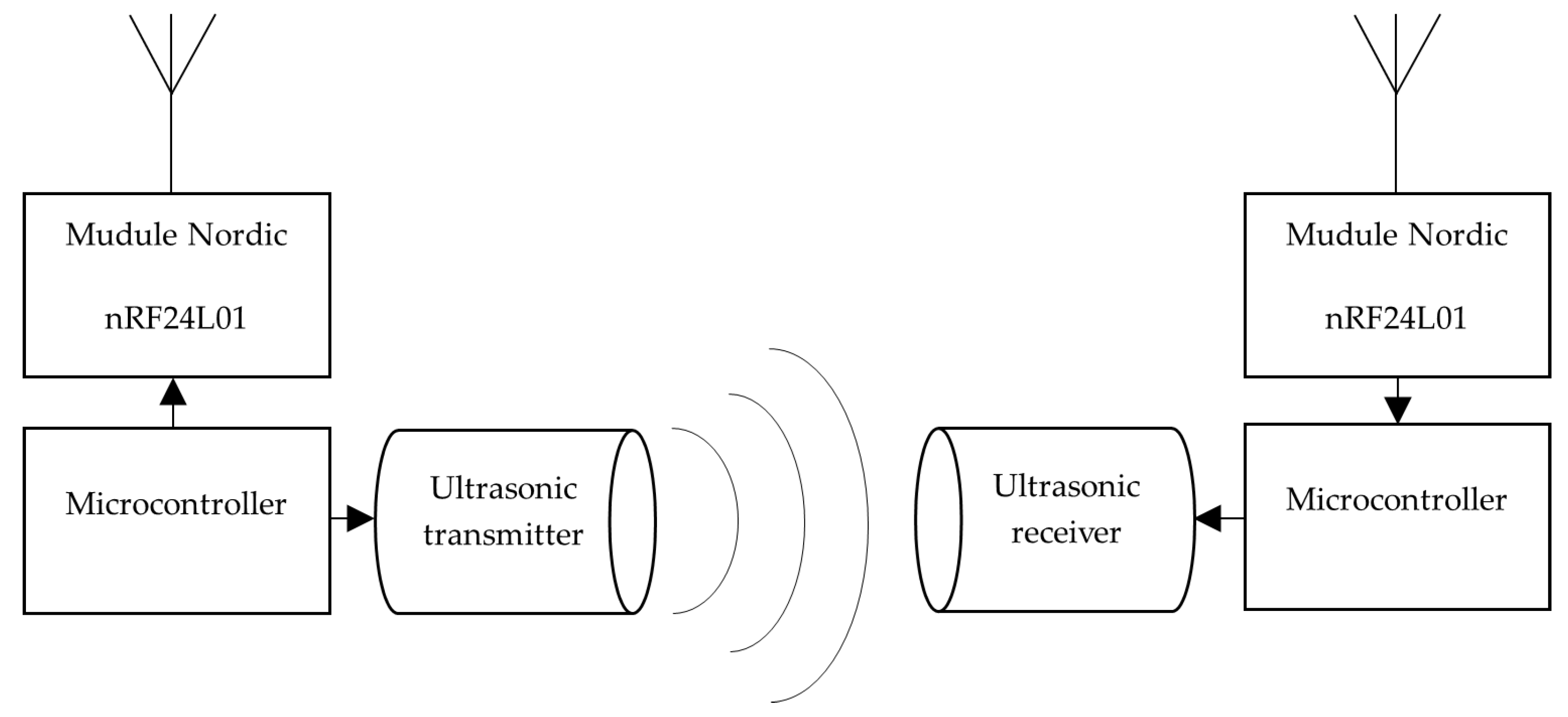
The proposed method of distributing triangular patterns of beacons is more demanding in terms of the number of beacons, but the beacons have only one transducer (unlike, for example, [23], where there are up to five transducers). This results in an beacon power consumption below 20 mA, which ensures trouble-free operation for at least 20 days using, for example, a 3S LiPo battery pack with a capacity of 1 Ah. Of course, the operating interval can be significantly extended by optimizing the processor’s operation during downtime or when the mobile robot is not working. These energy-independent beacons from central electrical power can be placed on the ceiling without additional wiring. The block diagram of the beacon and tag is shown in Figure 2.
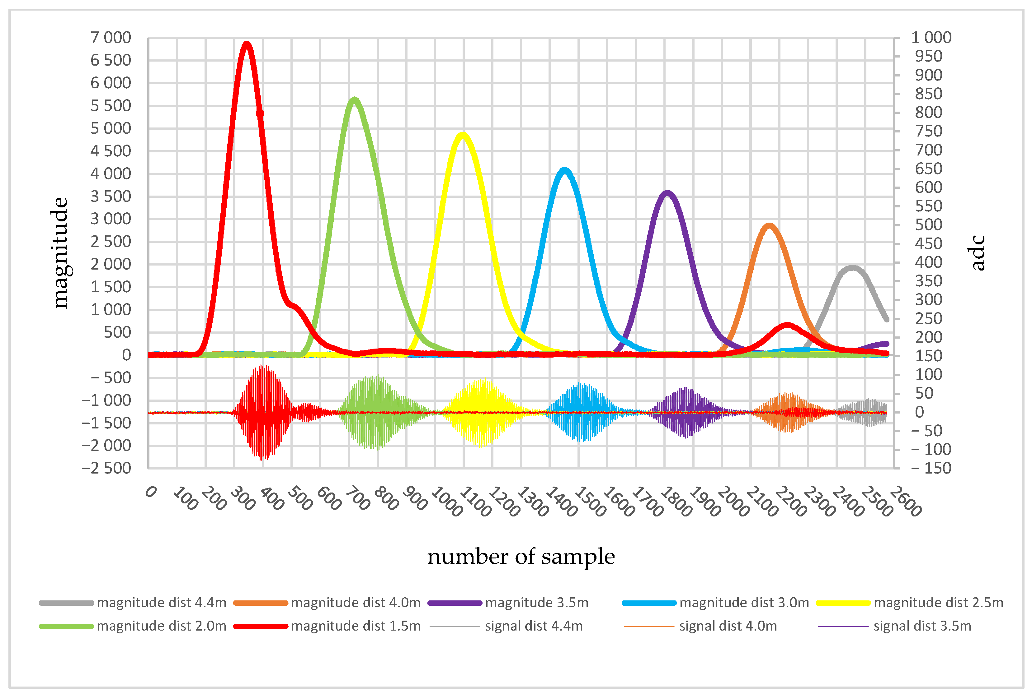
The tag must be capable of communicating and triggering the transmission of ultrasonic waves from the beacons at the most precise timing for synchronization. Communication is facilitated by the nRF24L01 module, which can be configured to ensure direct and clearly defined communication, where we can rely on known delays to minimally impact the resulting measurement (1 mm travels ultrasonic waves in less than 3 us under normal conditions). Control and data transmission settings are at a level where almost the entire data transmission is managed with the lowest possible delay interval and without any communication retries in case of data loss. In the event of data loss, the consciously controlling and computational microcontroller ensures communication retries. The STM32F303 microcontroller has been used for this purpose. The distance measurement process from the beacon to the tag proceeds as follows: The beacon always dictates the basic clock. It also determines which of the tags should send the ultrasonic signal. Therefore, synchronization is ensured using this principle. Now the RF signal is transmitted via the nRF module and the assumed delay for transmission and processing of the signal by the beacon, a timer for measurement is triggered in the tag. Meanwhile, in the beacon, the received HF signal is processed, and 20 periods of the ultrasonic signal with a frequency of 40 kHz are generated. The number of periods was determined through experimental verification, where multiple possibilities were tested. Using an oscilloscope, measurements of the envelope of the received signal on the ultrasonic receiver were taken for various distances from the ultrasonic transmitter. Specifically, the distances were 1.5, 2.5, and 3.5 m. For these distances, measurements were taken with different numbers of periods (10, 12, …, 40). For each distance, the maximum of the received signal envelope was evaluated. The maximum for periods less than 20 exhibited lower values than the maximum for 20 periods. For periods with values above 20, the maximum did not increase further, but there was an area where the derivative of the maximum was equal to zero at multiple points (not just one). Based on these measurements, the sufficient number of periods turned out to be exactly 20. After the time required for the ultrasonic signal to travel 1 m (dead zone not required) sent from the tag elapses, the tag starts sampling the ADC channel with a period of 4 microseconds. After collecting N all = 2700 samples, a fast Fourier transformation calculation is initiated in the microcontroller. The use of 2700 samples represent, under normal conditions, the passage of the ultrasonic signal approximately 3.75 m, so after adding the dead zone, we are able to evaluate the distance from 1 m to 4.75 m. Of course, considering the nature of the fast Fourier transform (FFT) calculation and signal evaluation after N = 125 samples, it is evident that the last approximately 175 cm is not calculated. It is not a problem to determine the distance up to 4.5 m, which fully satisfies our requirements for the typical type of buildings. Due to the sufficiently fast calculation, the step of evaluating the signal magnitude in the 40 kHz range from the collected samples was set to N/2. Lowering the step setting slightly increased repeatability and accuracy in experiments but significantly extended the FFT calculation time. When using a budget microcontroller STM clocked at 64 MHz and performing a simple FFT calculation, the computation takes 11.4 ms. This time, together with the sampling time (10.7 ms), communication time with the nRF module (0.2 ms), and the time needed for data collection delay (3 ms), determines the time required for evaluating the distance from a single beacon (25.3 ms). For detecting and evaluating distances from three beacons, a total time of 25.5 ms is required, which represents the sampling frequency for determining position as 13 Hz. Figure 3 presents the measured results for various distances.
The graph has been created from measurements for distances of 1.5, 2.0, 2.5, 3.0, 3.5, 4.0, and 4.4 m, representing the range where we expect robot position measurements to be necessary. Naturally, the measured values are in the ideal position, meaning that both the beacon and the tag are aligned. The horizontal axis in the graph represents the sample number, which are dimensionless, measured using the ADC. On the right side of the graph, there is a scale and axis values of the 8-bit signal from the ADC (−128; 127). The bottom part shows the received signals for different distances, displaying the outer envelope of the received signal and its profile. The left axis shows the FFT magnitude values for 40 kHz. The magnitude precedes the signal envelope by 125/2 samples, as evident from the calculation’s nature. The strength of the received ultrasonic signal decreases at higher distances. The signal is strongest, as well as its magnitude, for the shortest distance, i.e., 1.5 m, see in Figure 4.
During the measurements, the repeatability of the measurement principle was crucial, which can be determined using the standard deviation. This should ensure measurement accuracy after calibration to precise distances. Therefore, distances were only approximately set using a tape measure. For each approximate distance (as shown in Figure 3), the repeatability of the measurement was ultimately evaluated. The conversion of distance from the measured results was possible by creating an arithmetic progression method of calculated magnitudes for a given time interval. We could calculate the distance from the measured results by creating a graph from the arithmetic averages of magnitudes for each distance and then fitting a curve through the created points, letting MATLAB estimate the equation of the fitted curve. The second option, due to future calibration, was to create an equation that would also include the calculation of the speed of sound in air at a given temperature and humidity. The equation also includes the offset of the measurement start by the dead zone as well as the delay from the signal transmission, which in this case was a total of 2944 microseconds.
where magmax is the sample with the highest magnitude and the speed of ultrasound propagation in air for a known temperature and humidity is as follows:
where T is the temperature in °C and RH is the relative humidity of the air in %.
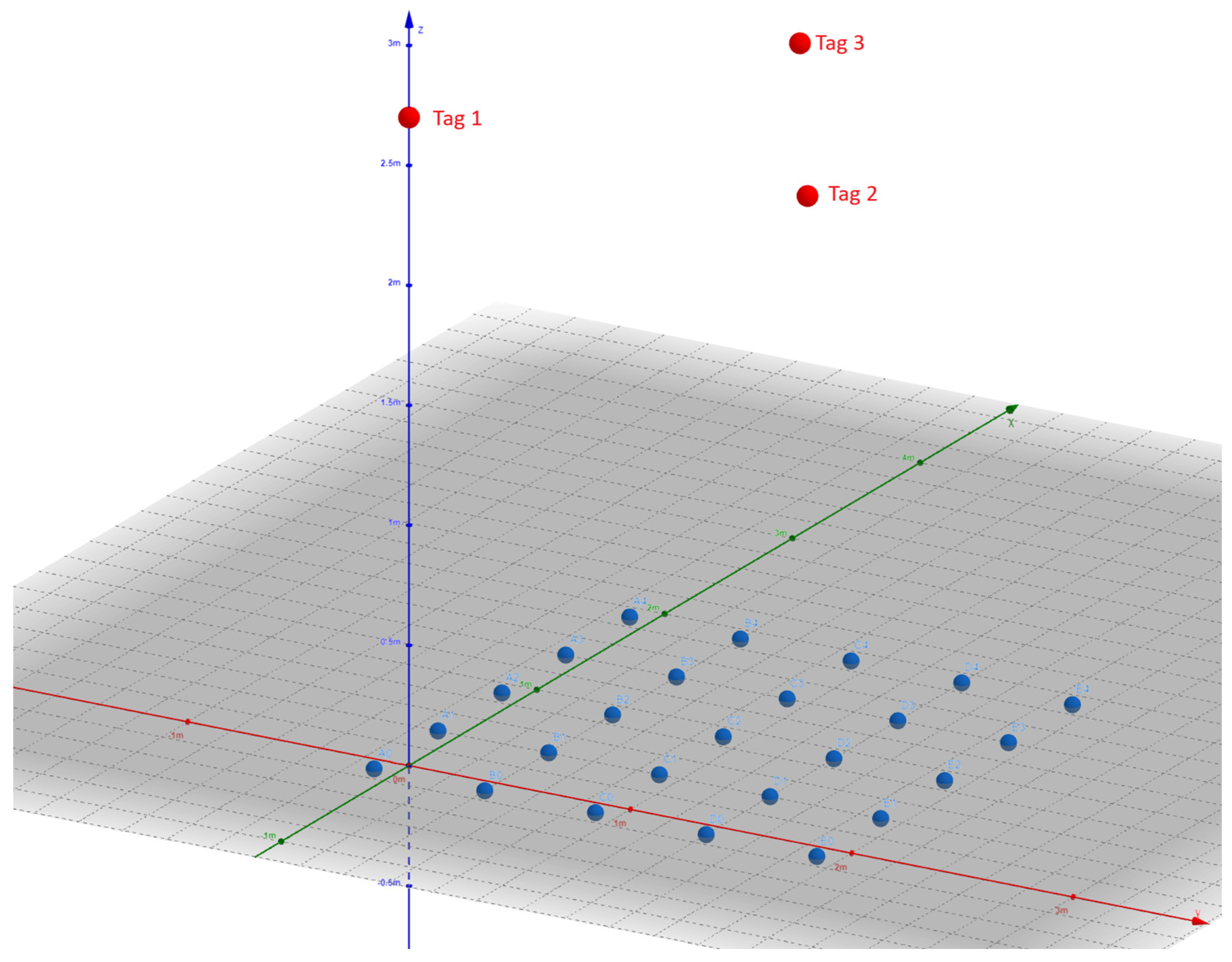
After calibrating all three tags with the receiver, we proceeded to verify the repeatability of the measurements and thus the accuracy for determining the position of the receiver in space. According to Figure 5, the system of three tags was mounted on the ceiling approximately using a tape measure.
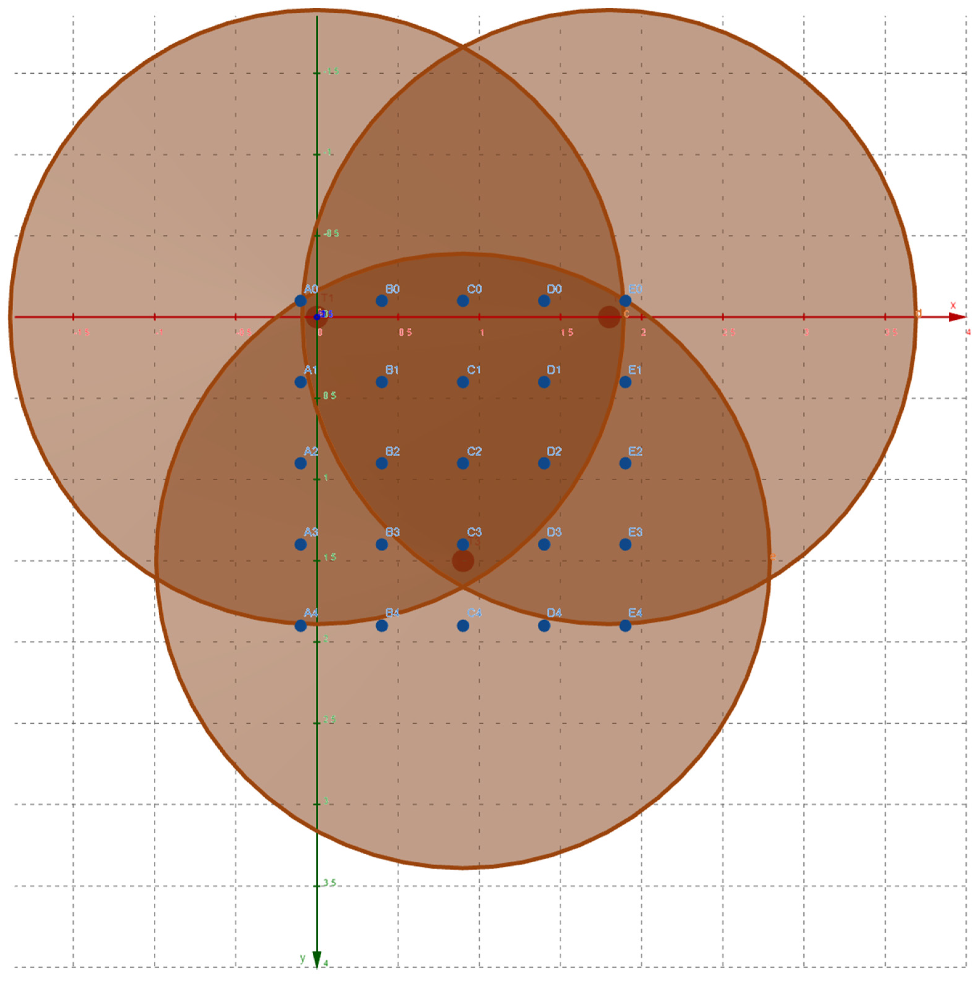
For testing purposes, a space with a ceiling height of more than 2.7 m was designed. By computing the beam angle of the transducer for losses up to −10 dB, the distance of the sides of the mounting triangle was calculated to be less than 2 m. Therefore, a specific length of sides, 1.8 m, was proposed, which falls within the calculated interval. The origin of the coordinate system was designed at point T1 (beacon 1), such that its x-axis passed through point T2 (beacon 2). Points T1 to T3 lie in a horizontal plane with the floor and ceiling. This plane is at the level of the ceiling. The axis, when viewed from above, points downward. Points A0 to E4 were marked on the floor for measurement purposes. Using the online tool GeoGebra, a model of the arrangement of elements in space was constructed to better determine the intersection of all three planes derived from the 70° angle beam and the height of the system in Figure 6.
For this specific case and for a height of 2.72 m (measuring height), the points B0, C0, D0, B1, C1, D1, B2, C2, D2, and C3 lie at the intersection of the circles from beacons 1, 2, and 3. The remaining points either intersect only two circles or are only inside one circle at Figure 7.
At points A0, A1, …, E4, repeated measurements were conducted. In each point, 100 measurements were taken. From the measurements using Equations (1) and (2), the distances from the receiver to beacons 1 to 3 were calculated. The coordinate system chosen was where the origin of the coordinate system is at point beaconT1 [0;0]. beaconT1 has coordinates x1 and y1, and beacon2 has coordinates x2 and y2. The x-axis passes through point beacon2, and the z-axis is downward. The basic equations for trilateration calculation of measured coordinates from distances d1, d2, and d3 are as follows:
where x, y, and z are coordination of the measuring point.
However, the mentioned equations have an error in the calculation, as the calculation for the x-coordinate does not take into account the intersection of all three distances. The coordinate is calculated only from distances d1 and d2. The calculation of the y and z axes is then derived from this. Therefore, it was appropriate to create calculations where the center of the coordinate system is also beacon2 and beacon3. Thus, using transformation (rotation and translation), both coordinate systems were recalculated into our chosen basic coordinate system with the center at point beacon1 and the x-axis passing through point beacon2. This created a system of equations for calculating the coordinates x, y, and z of the measured point. For calculating coordinates with the center at point beacon1 [0;0] and points beacon2 [1800;0] and beacon3 [900;1500], the equations are as follows:
Subsequently, for the coordinate system with the center at point beacon2 [0;0] and points beacon3 [1750;0] and beacon1 [925;1540], the equations are as follows:
Finally, for the coordinate system with the center at point beacon3 [0;0] and points beacon1 [1750;0] and beacon2 [825;1540], the equations are as follows:
It was mentioned that the base coordinate system is identical to the coordinate system where its center is at beacon1, and the x-axis passes through beacon2. From the above, it follows:
For the conversion of the coordinate system x″, y″, z″ to the base coordinate system, it was necessary to consider a transformation by rotation of 120.969° and a shift in the x-axis of −1800 mm in the calculation. The calculation of the coordinates is as follows:
For the conversion of the coordinate system x′′′, y′′′, z′′′ to the base coordinate system, it was necessary to consider a transformation by rotation of 120.969° and a shift in the x-axis of −900 mm and y-axis of −1500 mm. The calculation of the coordinates is as follows:
After the conversion, all distance samples in the measured point (100 samples) were calculated up to 300 coordinate results using the aforementioned trilateration. For each such measurement, the repeatability, and thus the possible accuracy at the given point, was calculated using the arithmetic mean and, especially, the standard deviation. The results were transferred to a table and graphs for better understanding.
4. Evaluation and Discussion
After applying the system to the ceiling of the experimental workplace (Figure 8), with an accuracy of +/−5 mm, measurements were conducted at all points from A0 to E4 (25 points).
At each point, 100 measurements of the tag length from each of the beacons were performed, meaning a total of 300 measurements were taken at each point. The beacons were synchronized and triggered exactly as they would be in the application, sequentially. Initially, a request for the first beacon (T1) came through via an HF signal. Subsequently, the beacon emitted an ultrasonic signal (40 kHz) lasting 20 periods. Using the Time of Flight (TOF) method, the processor in the tag evaluated the distance and sent a request to the next beacon (T2). This process was repeated 99 more times after measuring all three distances. Before the trilateration calculation, it was appropriate to verify the obtained results and evaluate the repeatability of distance measurements from the beacons at different points (Figure 9) using the standard deviation.
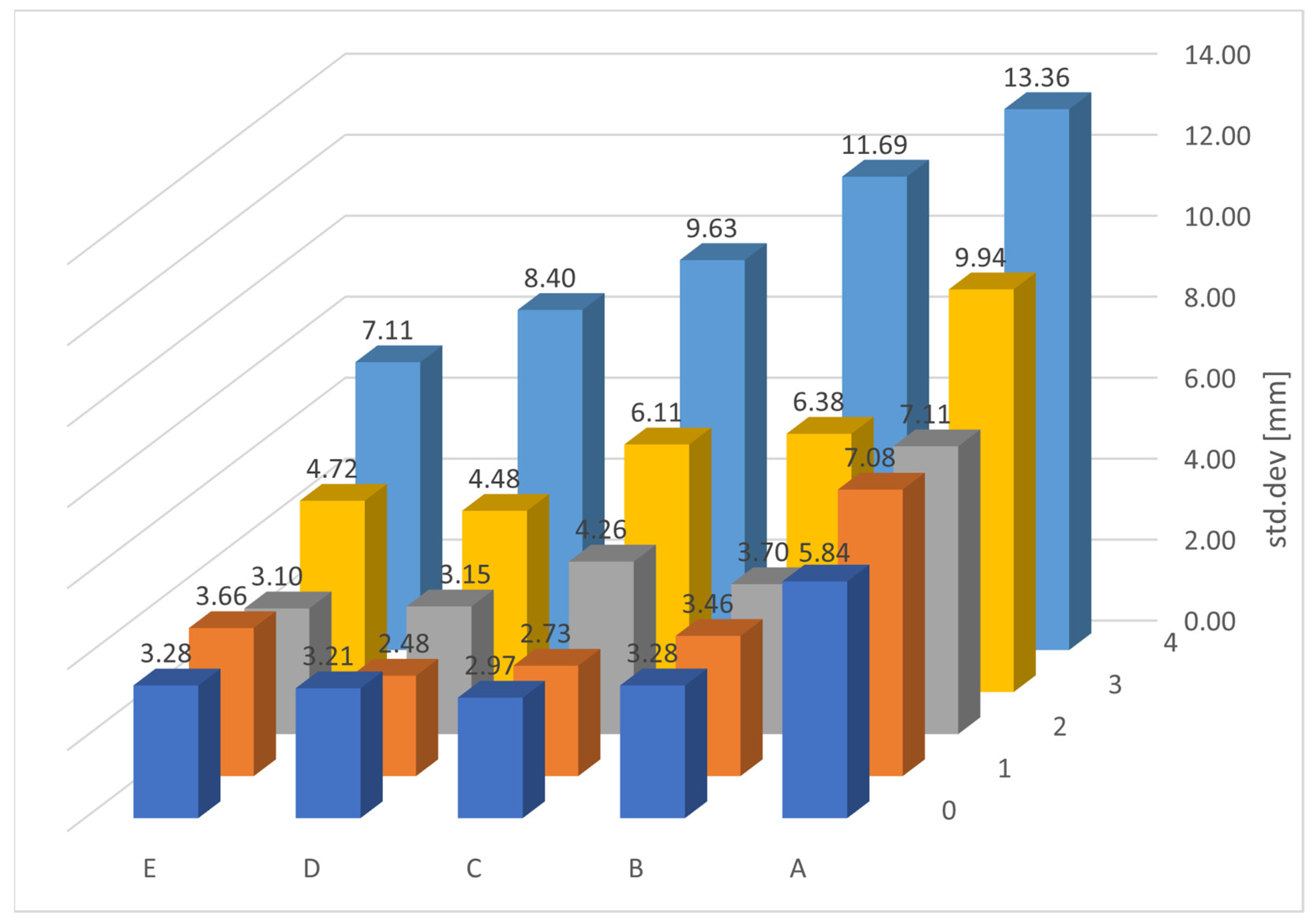
The table clearly displays, for each point, the average value (row AVG) of measured lengths from the beacons (columns distT1, distT2, distT3) and the standard deviation from the average value (±), which expresses the repeatability of distance measurements at individual points. The display of points A0 to E4 correlates with Figure 3, which is a top view of the measured points. Green color indicates points that fall within the relevant range according to Figure 5. Figure 10 shows the standard deviation view of the distance distT1.
The beacon was positioned at a height between points A0, A1, B0, and B1. In these points, which are closest to the ultrasonic transmission axis, the smallest standard deviations were measured (2.13 mm to 2.49 mm). The graph illustrates an increase in standard deviations as the measured points move farther from the ultrasonic transmission axis. The most unfavorable condition is observed at point E3 (16.92 mm). However, this point lies outside the area of good coverage by the signal from beacon T1. Among the points still within the signal coverage radius of this beacon, the highest standard deviation was recorded at point D2 (6.99 mm). Figure 11 displays the standard deviations of the measured distances distT2.
In this case, beacon T2 was positioned between points D0, D1, E0, and E1. In these points, there are also minimal standard deviations (2.48 mm to 3.66 mm). The following Figure 12 illustrates the standard deviations of distance measurements from beacon T3.
The graph is rotated 180° for better clarity. The beacon is located between points C3 and C4 (with standard deviations of 3.45 mm and 3.98 mm). The highest standard deviation was measured at point D0 (5.95 mm).
In [32], a similar distance measurement system using the TOF method with a variable signal period and utilizing significantly more expensive hardware for measurement is employed. The standard deviation in this system was measured at 0.7 mm, which is 3 to 10 times more precise compared to (2.13 mm to 6.99 mm) in this article’s system. However, the [32] system is not suitable for mobile robotics due to its dimensions. The distance measurement system using reflected ultrasonic signal measurement [33] achieves a distance measurement error of 13 mm to 234 mm. The system presented in this article exhibits a distance measurement error in valid measured points ranging from 6 mm to 21 mm.
From the measured distances using trilateration calculations (Equations (6)–(23)), average coordinate values (row AVG) for x, y, and z measurements were computed for each point (Figure 13).
The standard deviation of coordinates x, y, and z is expressed in the row “±”. The nature of the measurement confirmed the assumption that the smallest standard deviations would be observed in the z-axis. The highest standard deviation was found at points A4 and E4, which is precisely as expected. The standard deviation at these points is
13.42 mm and 13.79 mm, respectively. Regarding the relevant range (green) from the intersections of all three radii, the standard deviation ranges from 1.83 mm to 3.28 mm. The trend of computed values is depicted in Figure 14.
In the x and y axes, the assumption was for worse results compared to the z-axis. The standard deviations plotted on the graph for the x-axis are shown in Figure 15.
Here, the standard deviations range between 6.49 mm (B0) and 14.69 mm (C3). The standard deviations plotted in the graph for the y-axis are shown in Figure 16.
Similarly, to the y-axis, it was anticipated that the worst results would come from points outside the valid range for the x-axis.
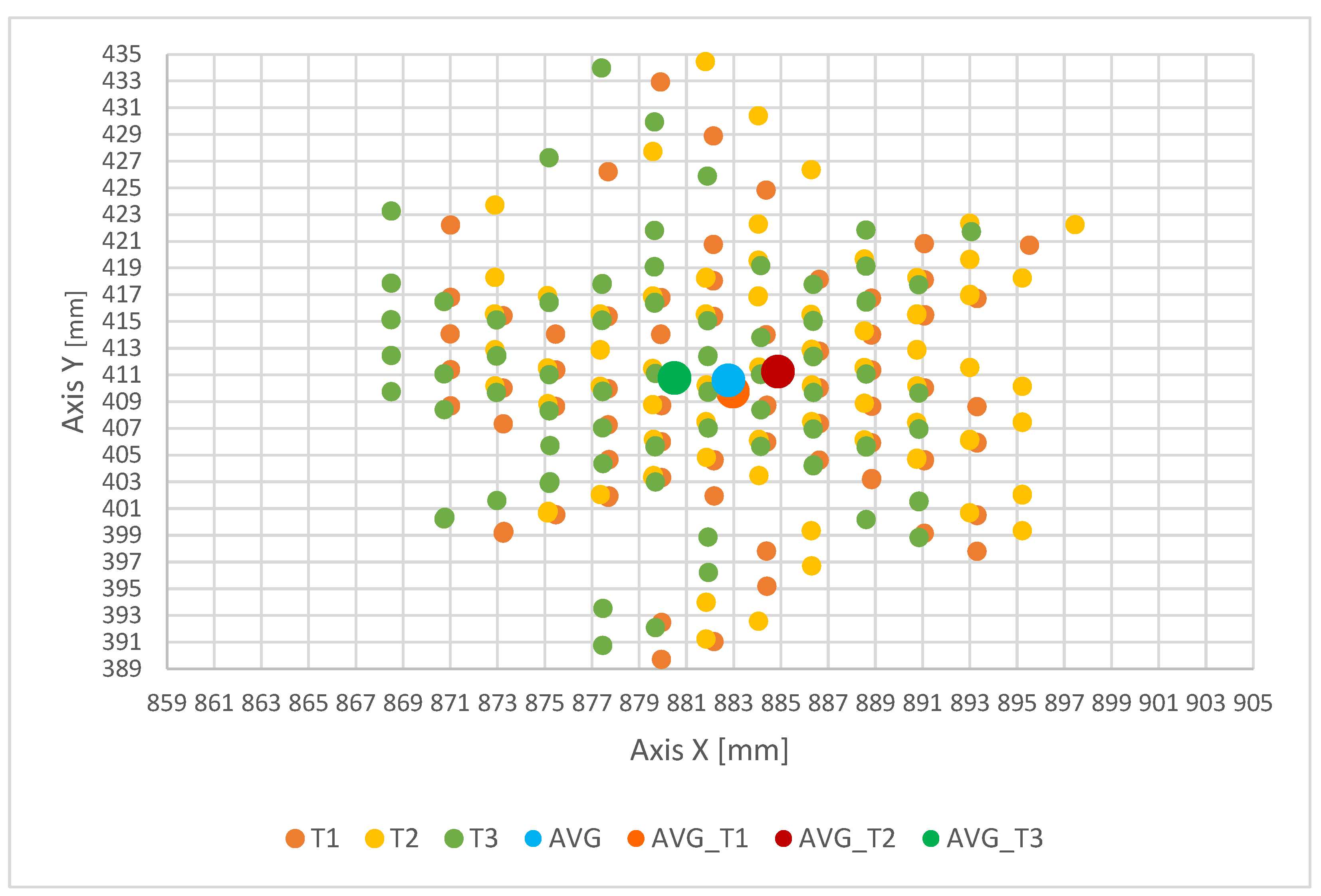
For the selected point C1, located within the valid range, a cloud of the occurrence of computed coordinate values from all measured values is displayed. Since the measured distance values are discrete, this is also reflected in the computed values, which exhibit some rasterization shown in Figure 17.
The graph depicts the variance of measured values as well as their arithmetic averages. For better visualization and to ensure that values do not create clusters located outside of the other values due to transformations, the occurrence of points is displayed in different colors depending on the original coordinate system. Additionally, the overall arithmetic average (blue) and the arithmetic averages of the calculated values from transformations are shown. Compared to system [34], which is similar to the presented design, the system exhibits similar standard deviations in individual axes (9.45 mm in the x-axis, 11.28 in the y-axis, 7.01 in the z-axis).
As indicated, for example, in [35], the use of BLE for indoor positioning includes methods based on signal strength fingerprinting, which significantly increases localization accuracy in conditions where direct line-of-sight to the beacon is limited. The system can be quite accurate for certain applications but may not meet the requirements of applications that demand high precision. The maximum error is approximately 1.3 m, and the minimum positioning error ranges from approximately 6 cm to over 85 cm depending on the specific position and the function used.
5. Conclusions
The presented system, designed for indoor localization of mobile robots and inventory management (Figure 1), meets the requirements of RTLS, has a sampling frequency >10 Hz, and is simple, easily deployable, and cost-effective. It also fulfills the assumption of measurement repeatability in individual axes <20 mm. From the measured and calculated results, the worst outcome within the valid range was 14.69 mm for the x-coordinate and 10.87 mm for the y-coordinate. Results for the z-axis are less significant due to the nature of mobile robot movement, where this axis is mostly unnecessary as its value remains constant. However, further verification of the proposed system is necessary, involving measurements in precise positions focusing on the deviation from the actual position, to determine deviations from actual positions at measurement points. It is necessary to construct a stand that allows precise positioning of the receiver and enables the attachment of tags with high precision relative to each other and to the measurement points. Additionally, verification of the system during changes in movement and its detection within the valid area is required. Therefore, subsequent studies delved into the subject of dynamic testing, where the variability of conditions in complex indoor spaces can affect signal transmission due to reflection or absorption of ultrasonic waves. Moving objects, such as people or other robots, can distort data due to Doppler effects, requiring data processing algorithms to adapt to changes. Precise time synchronization becomes critical, as delays in signal processing significantly affect localization accuracy. Challenges associated with multiple signal paths require the development of methods to distinguish the primary signal from reflections. Also, there is an increasing need for faster data updates for effective operation in dynamic conditions.
Author Contributions
Conceptualization, M.S. and M.G.; methodology, M.S. and R.J.; software, M.S.; validation, J.S.; data curation, M.G.; writing—review and editing, M.G.; visualization, J.S.; supervision, M.S. All authors have read and agreed to the published version of the manuscript.
Funding
This research was funded by Cultural and Education Grant Agency grant number KEGA: 020TUKE-4/2022 and Science Grant Agency grant number VEGA: 1/0215/23 and VEGA: 1/0215/24.
Institutional Review Board Statement
Not applicable.
Informed Consent Statement
Not applicable.
Data Availability Statement
The original data presented in the study are available at http://www.sjf.tuke.sk/kr/images/download/Measred_data.xlsx.
Acknowledgments
This research was supported by project KEGA: 020TUKE-4/2022 Development and implementation of new approaches in teaching industrial and collaborative robotics and VEGA: 1/0215/23 Research and development of robotic workplaces equipped with industrial and collaborative robots and VEGA: 1/0294/24 Research and development of a multi-robotic system with distributed intelligence in the cloud.
Conflicts of Interest
The authors declare no conflicts of interest.
References
- Zafari, F.; Gkelias, A.; Leung, K.K. A Survey of Indoor Localization Systems and Technologies. IEEE Commun. Surv. Tutor. 2019, 21, 2568–2599. [Google Scholar] [CrossRef]
- Duchoň, F. Mobile Robots Controlling; FELIA: Bratislava, Slovakia, 2023; ISBN 978-80-89824-14-4. [Google Scholar]
- Grytsiv, M. Simulation of the Trajectory of a Mobile Robot in Flowcode. Master’s Thesis, Technical University of Kosice, Kosice, Slovakia, 2020. Available online: https://opac.crzp.sk/?fn=detailBiblioForm&sid=F5195A1FF5FC8574514BA0DFA517 (accessed on 22 January 2024).
- Li, J.; Han, G.; Zhu, C.; Sun, G. An Indoor Ultrasonic Positioning System Based on TOA for Internet of Things. Mob. Inf. Syst. 2016, 2016, 4502867. [Google Scholar] [CrossRef]
- Kunhoth, J.; Karkar, A.; Al-Maadeed, S.; Al-Ali, A. Indoor positioning and wayfinding systems: A survey. Hum.-Centric Comput. Inf. Sci. 2020, 10, 18. [Google Scholar] [CrossRef]
- Hee, L.G.; Marcelo, H.A. Mobile Robots Navigation, Mapping, and Localization Part I. In Encyclopedia of Artificial Intelligence; IGI Global: Hershey, PA, USA, 2008; ISBN 9781599048499. [Google Scholar] [CrossRef]
- Yurevich, E.I. Sensor Systems in Robotics; Polytechnic University Publishing House: Sankt Peterburg, Russia, 2013; ISBN 978574223774-7. [Google Scholar]
- GPS. Available online: https://en.wikipedia.org/wiki/GPS (accessed on 22 January 2024).
- Galileo. Available online: https://en.wikipedia.org/wiki/Galileo_(satellite_navigation) (accessed on 22 January 2024).
- GlONASS. Available online: https://montrans.ru/blog/sistema-glonass (accessed on 22 January 2024).
- Farid, Z.; Nordin, R.; Ismail, M.; Al-Ali, A. Recent Advances in Wireless Indoor Localization Techniques and System: A survey. J. Comput. Netw. Commun. 2013, 2013, 185138. [Google Scholar] [CrossRef]
- Turgut, Z.; Aydin, G.Z.G.; Al-Ali, A. Indoor Localization Techniques for Smart Building Environment: A survey. Procedia Comput. Sci. 2016, 83, 1176–1181. [Google Scholar] [CrossRef]
- Md Din, M.; Jamil, N.; Maniam, J.; Mohamed, M.A. Review of indoor localization techniques: A survey. Procedia Comput. Sci. 2018, 7, 201–204. [Google Scholar] [CrossRef]
- Obeidat, H.; Shuaieb, W.; Obeidat, O.; Abd-Alhameed, R. A Review of Indoor Localization Techniques and Wireless Technologies: A survey. Wirel. Pers. Commun. 2021, 119, 289–327. [Google Scholar] [CrossRef]
- Webster, J.G.; Shuaieb, W.; Obeidat, O.; Abd-Alhameed, R. Robot Localization: An Introduction. In Wiley Encyclopedia of Electrical and Electronics Engineering: A Survey; John Wiley & Sons: Hoboken, NJ, USA, 2021. [Google Scholar] [CrossRef]
- Panigrahi, P.K.; Bisoy, S.K.; Obeidat, O.; Abd-Alhameed, R. Localization strategies for autonomous mobile robots: A review. J. King Saud Univ.-Comput. Inf. Sci. 2022, 34, 6019–6039. [Google Scholar] [CrossRef]
- Wang, J.; Takahashi, Y.; Obeidat, O.; Abd-Alhameed, R. Indoor mobile robot self-localization based on a low-cost light system with a novel emitter arrangement: A review. ROBOMECH J. 2018, 5, 6019–6039. [Google Scholar] [CrossRef]
- Crețu-Sîrcu, A.L.; Schiøler, H.; Cederholm, J.P.; Sîrcu, I.; Schjørring, A.; Larrad, I.R.; Berardinelli, G.; Madsen, O. Evaluation and Comparison of Ultrasonic and UWB Technology for Indoor Localization in an Industrial Environment. Sensors 2022, 22, 2927. [Google Scholar] [CrossRef] [PubMed]
- Andreev, P.I.; Dobrzhansky, O.O. Mapping and Localization of Mobile Robots in a Non-Static Environment; Industrial and mobile robotics; Zhytomyr Polytechnic State University: Zhytomyr, Ukraine, 2020; pp. 175–176. [Google Scholar]
- UWB Technology for Wayfinding. Available online: https://www.tirichlabs.com/blog/uwb-technology-for-wayfinding/ (accessed on 24 January 2024).
- Indoor Positioning with Ultra-Wideband. Available online: https://www.infsoft.com/basics/positioning-technologies/ultra-wideband/ (accessed on 30 January 2024).
- Bluetooth® Low Energy (LE). Available online: https://www.bluetooth.com/learn-about-bluetooth/tech-overview/ (accessed on 10 January 2024).
- Anchor 5.0. Localino. Available online: https://localino.net/products-and-services/anchor5_0 (accessed on 14 January 2024).
- Indoor GPS. Available online: https://marvelmind.com/pics/marvelmind_presentation.pdf (accessed on 18 January 2024).
- Othman, W.; Gromov, V.S. Research of visual simultaneous localization and mapping-based navigation system for mobile robots. Sci. Tech. J. Inf. Technol. Mech. Opt. 2020, 20, 371–376. [Google Scholar] [CrossRef]
- Study of SLAM Methods for Indoor Navigation of a Mobile Robot. R2 Robotics Research Experience. 2021. Available online: https://habr.com/ru/post/560856/ (accessed on 5 January 2024).
- Hajduk, M.; Sukop, M. Multiagents System with Dynamic Box Change for MiroSot. In Proceedings of the 12th International FIRA RoboWorld Congress, Incheon, Republic of Korea, 16–18 August 2009; Springer: New York, NY, USA, 2009; Volume 44, pp. 287–292, ISBN 978-3-642-03985-0. [Google Scholar]
- Janos, R.; Sukop, M.; Semjon, J.; Vagas, M.; Galajdova, A.; Tuleja, P.; Koukolová, L.; Marcinko, P. Conceptual design of a leg-wheel chassis for rescue operations. Int. J. Adv. Robot. Syst. 2017, 14, 1–9. [Google Scholar] [CrossRef]
- Jánoš, R.; Sukop, M.; Semjon, J.; Tuleja, P.; Marcinko, P.; Kočan, M.; Grytsiv, M.; Vagaš, M.; Miková, Ľ.; Kelemenová, T. Stability and Dynamic Walk Control of Humanoid Robot for Robot Soccer Player. Machines 2022, 10, 463. [Google Scholar] [CrossRef]
- Saravanakumar, Y.N.; Sultan, M.T.H.; Shahar, F.S.; Giernacki, W.; Łukaszewicz, A.; Nowakowski, M.; Holovatyy, A.; Stępień, S. Power Sources for Unmanned Aerial Vehicles: A State-of-the Art. Appl. Sci. 2023, 13, 11932. [Google Scholar] [CrossRef]
- Silarski, M.; Nowakowski, M. Performance of the SABAT Neutron-Based Explosives Detector Integrated with an Unmanned Ground Vehicle: A Simulation Study. Sensors 2022, 22, 9996. [Google Scholar] [CrossRef] [PubMed]
- Carotenuto, R.; Merenda, M.; Iero, D.; Corte, F.G.D. Ranging RFID Tags With Ultrasound. IEEE Sens. J. 2018, 18, 2967–2975. [Google Scholar] [CrossRef]
- Hoeflinger, F.; Saphala, A.; Schott, D.J.; Reindl, L.M.; Schindelhauer, C. Passive Indoor-Localization using Echoes of Ultrasound Signals. In Proceedings of the 2019 International Conference on Advanced Information Technologies (ICAIT), Yangon, Myanmar, 6–7 November 2019; pp. 60–65. [Google Scholar] [CrossRef]
- Kapoor, R.; Ramasamy, S.; Gardi, A.; Bieber, C.; Silverberg, L.; Sabatini, R. A Novel 3D Multilateration Sensor Using Distributed Ultrasonic Beacons for Indoor Navigation. Sensors 2016, 16, 1637. [Google Scholar] [CrossRef] [PubMed]
- Benaissa, B.; Hendrichovsky, F.; Yishida, K.; Koppen, M.; Sincak, P. Phone Application for Indoor Localization Based on Ble Signal Fingerprint. In Proceedings of the 2018 9th IFIP International Conference on New Technologies, Mobility and Security (NTMS), Paris, France, 26–28 February 2018; pp. 1–5. [Google Scholar] [CrossRef]
Figure 1.
The layout of the basic tag pattern relative to the room dimensions.

Figure 2.
Ultrasound measurement principle.

Figure 3.
Measured signal at different distances and its FFT magnitude for 40 kHz.

Figure 4.
Measured signal at distance 1.5 m and its FFT magnitude for 40 kHz.

Figure 5.
Arrangement of tags and measured points when viewed from above.

Figure 6.
Model created by GeoGebra.

Figure 7.
Displaying circles and their intersections for individual beacons and a height of 2.72 m above the measured plane.
Figure 7.
Displaying circles and their intersections for individual beacons and a height of 2.72 m above the measured plane.

Figure 8.
(a) Beacons on the ceiling, (b) tag.

Figure 9.
Arithmetic averages of distances and their standard deviations measured at points A0 to E4 using our measurement system.
Figure 9.
Arithmetic averages of distances and their standard deviations measured at points A0 to E4 using our measurement system.

Figure 10.
Standard deviations of measurements of distances from T1.

Figure 11.
Standard deviations of measurements of distances from T2.

Figure 12.
Standard deviations of measurements of distances from T3.

Figure 13.
Arithmetic averages of coordinates and their standard deviations measured at points A0 to E4.
Figure 13.
Arithmetic averages of coordinates and their standard deviations measured at points A0 to E4.

Figure 14.
Standard deviations of the z-coordinate.

Figure 15.
Standard deviations of the x-coordinate.

Figure 16.
Standard deviations of the y-coordinate.

Figure 17.
Cloud of calculated points from measurements displayed in the x and y axes for point C1 (top view).
Figure 17.
Cloud of calculated points from measurements displayed in the x and y axes for point C1 (top view).


Table 1.
Comparisons between different technologies [18].
Table 1.
Comparisons between different technologies [18].
| Year | System | Room Size m2/ Environment | LOS/ NLOS/ Mix | 2D Accuracy [m] Mean ± Std |
|---|---|---|---|---|
| 2014 | 802.15.4a compliant UWB System | 5.3 × 11.5/ Office | LOS (Static) | <0.4 ± 0.04 |
| LOS (Dynamic) | 0.89 ± 0.08 | |||
| NLOS (Dynamic) | 0.88 ± 0.1 | |||
| 2016 | ATLAS | Laboratory | LOS | 0.21 |
| 2017 | BeSpoon | 12 × 12/Industrial | Mix | 0.71 |
| Ubisense | Laboratory | 1.10 | ||
| DecaWave | 0.49 | |||
| 2019 | Pozyx | Industrial | LOS (1.5 m) | 1.5 ± 0.03 |
| Laboratory | NLOS (1.5 m) | 1.75 ± 0.03 | ||
| LOS (10.9 m) | 11.6 ± 1.7 | |||
| NLOS (10.9 m) | 11.6 ± 4.4 | |||
| 2019 | TimeDomain PulsON440 | Galvanic Industry | LOS (Static) | 0.38 |
| NLOS (Static) | 0.22 | |||
| 2019 | Pozyx | Industrial Laboratory | LOS | 0.22 |
| NLOS | >1 | |||
| 2020 | DecaWave | Industrial Laboratory | LOS (Static) | 0.01 ± 0.01 |
| 1997 | Active BAT | Office | LOS | 0.03 |
| 1998 | Prototype | 0.5 × 0.4 | LOS (Static) | 0.04 ± 0.01 |
| 2000 | MIT Cricket | Office | LOS | 0.1 |
| 2003 | DOLPHIN | Office | LOS | |
| 2010 | LOSNUS | Office | LOS (Static) | 0.001 |
| 2011 | Prototype | 1.2 × 1.8 m | LOS (Static) | 0.03 |
| 2016 | Prototype | Laboratory | LOS (Static) | 0.02 |
| 2017 | Prototype | Laboratory | LOS (Dynamic) | 0.012 |
| 2019 | Decawave TREK1000 (UWB) Locate-US (US) | 24 × 14/ Industrial Laboratory | Mix (Static) | <0.2 (UWB and US) |
| Mix (Dynamic- robot) | <0.2 (US) <0.12 (UWB) | |||
| Mix (Dynamic- moving person) | <0.65 (US) >0.5 (UWB) |
Disclaimer/Publisher’s Note: The statements, opinions and data contained in all publications are solely those of the individual author(s) and contributor(s) and not of MDPI and/or the editor(s). MDPI and/or the editor(s) disclaim responsibility for any injury to people or property resulting from any ideas, methods, instructions or products referred to in the content. |
© 2024 by the authors. Licensee MDPI, Basel, Switzerland. This article is an open access article distributed under the terms and conditions of the Creative Commons Attribution (CC BY) license (https://creativecommons.org/licenses/by/4.0/).
Share and Cite
MDPI and ACS Style
Sukop, M.; Grytsiv, M.; Jánoš, R.; Semjon, J. Simple Ultrasonic-Based Localization System for Mobile Robots. Appl. Sci. 2024, 14, 3625. https://0-doi-org.brum.beds.ac.uk/10.3390/app14093625
AMA Style
Sukop M, Grytsiv M, Jánoš R, Semjon J. Simple Ultrasonic-Based Localization System for Mobile Robots. Applied Sciences. 2024; 14(9):3625. https://0-doi-org.brum.beds.ac.uk/10.3390/app14093625
Chicago/Turabian StyleSukop, Marek, Maksym Grytsiv, Rudolf Jánoš, and Ján Semjon. 2024. "Simple Ultrasonic-Based Localization System for Mobile Robots" Applied Sciences 14, no. 9: 3625. https://0-doi-org.brum.beds.ac.uk/10.3390/app14093625
Note that from the first issue of 2016, this journal uses article numbers instead of page numbers. See further details here.