
Enhancing Interpretability in Drill Bit Wear Analysis through Explainable Artificial Intelligence: A Grad-CAM Approach

Abstract
:1. Introduction
2. Background Theories
2.1. Convolutional Neural Networks
2.2. Gradient Class Activation Mapping
3. Materials and Methods
3.1. Data Collection and Preprocessing
3.2. Vibration Signal Analysis
3.3. Statistical Analysis
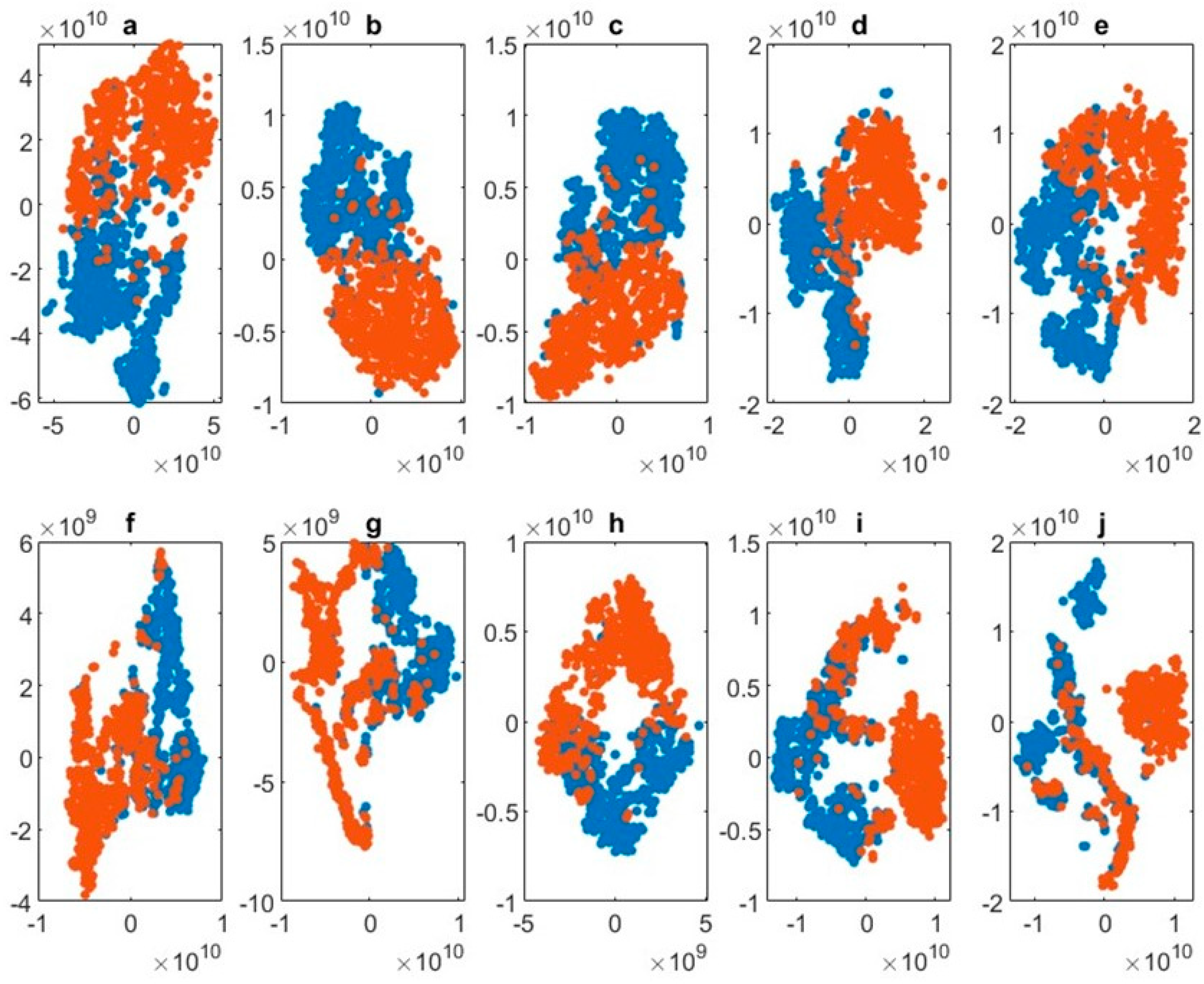
3.4. t-SNE Evaluation
3.5. Hyperparameter Tuning and Evaluation Metrics
4. Results
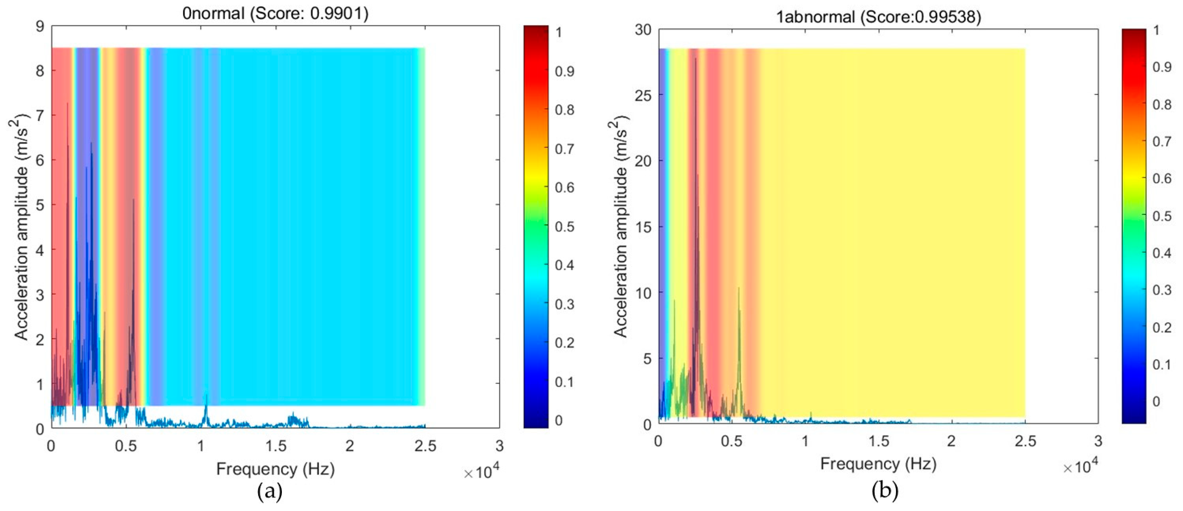
Interpretability with GradCAM
5. Discussion
6. Conclusions
Author Contributions
Funding
Institutional Review Board Statement
Informed Consent Statement
Data Availability Statement
Acknowledgments
Conflicts of Interest
References
- Nacib, L.; Saad, S.; Sakhara, S. A Comparative Study of Various Methods of Gear Faults Diagnosis. J. Fail. Anal. Prev. 2014, 14, 645–656. [Google Scholar] [CrossRef]
- Jaros, R.; Byrtus, R.; Dohnal, J.; Danys, L.; Baros, J.; Koziorek, J.; Zmij, P.; Martinek, R. Advanced Signal Processing Methods for Condition Monitoring. Arch. Comput. Methods Eng. 2023, 30, 1553–1577. [Google Scholar] [CrossRef]
- Nguyen, C.D.; Prosvirin, A.; Kim, J.-M. A Reliable Fault Diagnosis Method for a Gearbox System with Varying Rotational Speeds. Sensors 2020, 20, 3105. [Google Scholar] [CrossRef]
- Jardine, A.K.; Lin, D.; Banjevic, D. A review on machinery diagnostics and prognostics implementing condition-based maintenance. Mech. Syst. Signal Process. 2006, 20, 1483–1510. [Google Scholar] [CrossRef]
- Mohd Ghazali, M.H.; Rahiman, W. Vibration Analysis for Machine Monitoring and Diagnosis: A Systematic Review. Shock Vib. 2021, 2021, 9469318. [Google Scholar] [CrossRef]
- Ambhore, N.; Kamble, D.; Chinchanikar, S.; Wayal, V. Tool Condition Monitoring System: A Review. Mater. Today Proc. 2015, 2, 3419–3428. [Google Scholar] [CrossRef]
- Netzer, M.; Palenga, Y.; Fleischer, J. Machine tool process monitoring by segmented timeseries anomaly detection using subprocess-specific thresholds. Prod. Eng. 2022, 16, 597–606. [Google Scholar] [CrossRef]
- Oberst, U. The Fast Fourier Transform. SIAM J. Control Optim. 2007, 46, 496–540. [Google Scholar] [CrossRef]
- Messaoud, L. Drilling technology in mining industry. Energy J. 2006, 1, 5. [Google Scholar]
- Prasad, B.S.; Murthy, V.; Pandey, S. Investigations on rock drillability applied to underground mine development vis-à-vis drill selection. In Proceedings of the Conference on Recent Advances in Rock Engineering (RARE 2016), Bengaluru, India, 16–18 November 2016; Atlantis Press: Bengaluru, India, 2016. [Google Scholar] [CrossRef]
- Gómez, M.P.; Hey, A.M.; Ruzzante, J.E.; D’attellis, C.E. Tool wear evaluation in drilling by acoustic emission. Phys. Procedia 2010, 3, 819–825. [Google Scholar] [CrossRef]
- Katiyar, P.K.; Maurya, R.; Singh, P.K. Failure Behavior of Cemented Tungsten Carbide Materials: A Case Study of Mining Drill Bits. J. Mater. Eng. Perform. 2021, 30, 6090–6106. [Google Scholar] [CrossRef]
- Tian, J.; Fan, C.; Zhang, T.; Zhou, Y. Rock breaking mechanism in percussive drilling with the effect of high frequency torsional vibration. Energy Sources Part A Recovery Util. Environ. Eff. 2022, 44, 2520–2534. [Google Scholar] [CrossRef]
- Iqbal, M.; Madan, A.K. CNC Machine-Bearing Fault Detection Based on Convolutional Neural Network Using Vibration and Acoustic Signal. J. Vib. Eng. Technol. 2022, 10, 1613–1621. [Google Scholar] [CrossRef]
- Ben Ali, J.; Fnaiech, N.; Saidi, L.; Chebel-Morello, B.; Fnaiech, F. Application of empirical mode decomposition and artificial neural network for automatic bearing fault diagnosis based on vibration signals. Appl. Acoust. 2015, 89, 16–27. [Google Scholar] [CrossRef]
- Rhif, M.; Ben Abbes, A.; Farah, I.R.; Martínez, B.; Sang, Y. Wavelet Transform Application for/in Non-Stationary Time-Series Analysis: A Review. Appl. Sci. 2019, 9, 1345. [Google Scholar] [CrossRef]
- Li, Y.; Wang, J.; Shan, Y.; Wang, C.; Hu, Y. Measurement and Analysis of Downhole Drill String Vibration Signal. Appl. Sci. 2021, 11, 11484. [Google Scholar] [CrossRef]
- Rafezi, H.; Hassani, F. Drilling signals analysis for tricone bit condition monitoring. Int. J. Min. Sci. Technol. 2021, 31, 187–195. [Google Scholar] [CrossRef]
- Karakus, M.; Perez, S. Acoustic emission analysis for rock–bit interactions in impregnated diamond core drilling. Int. J. Rock Mech. Min. Sci. 2014, 68, 36–43. [Google Scholar] [CrossRef]
- Kawamura, Y.; Jang, H.D.; Hettiarachchi, D.; Takarada, Y.; Okawa, H.; Shibuya, T. A Case Study of Assessing Button Bits Failure through Wavelet Transform Using Rock Drilling Induced Noise Signals. J. Powder Metall. Min. 2017, 6, 162. [Google Scholar] [CrossRef]
- Qin, M.; Wang, K.; Pan, K.; Sun, T.; Liu, Z. Analysis of signal characteristics from rock drilling based on vibration and acoustic sensor approaches. Appl. Acoust. 2018, 140, 275–282. [Google Scholar] [CrossRef]
- Rafezi, H.; Hassani, F. Drill bit wear monitoring and failure prediction for mining automation. Int. J. Min. Sci. Technol. 2023, 33, 289–296. [Google Scholar] [CrossRef]
- Soleimani, M.; Campean, F.; Neagu, D. Diagnostics and prognostics for complex systems: A review of methods and challenges. Qual. Reliab. Eng. Int. 2021, 37, 3746–3778. [Google Scholar] [CrossRef]
- Senjoba, L.; Ikeda, H.; Toriya, H.; Hisada, M.; Adachi, T.; Kawamura, Y. Visualization of 1D CNN Lithology Identification Model from Rotary Percussion Drilling Vibration Signals Using Explainable Artificial Intelligence Grad-CAM. Int. J. Soc. Mater. Eng. Resour. 2022, 25, 224–228. [Google Scholar] [CrossRef]
- Kumar, C.; Vardhan, H.; Murthy, C.; Karmakar, N. Estimating rock properties using sound signal dominant frequencies during diamond core drilling operations. J. Rock Mech. Geotech. Eng. 2019, 11, 850–859. [Google Scholar] [CrossRef]
- Senjoba, L.; Sasaki, J.; Kosugi, Y.; Toriya, H.; Hisada, M.; Kawamura, Y. One-Dimensional Convolutional Neural Network for Drill Bit Failure Detection in Rotary Percussion Drilling. Mining 2021, 1, 297–314. [Google Scholar] [CrossRef]
- Lin, C.-J.; Jhang, J.-Y. Bearing Fault Diagnosis Using a Grad-CAM-Based Convolutional Neuro-Fuzzy Network. Mathematics 2021, 913, 1502. [Google Scholar] [CrossRef]
- Gao, Y.; Liu, J.; Li, W.; Hou, M.; Li, Y.; Zhao, H. Augmented Grad-CAM++: Super-Resolution Saliency Maps for Visual Interpretation of Deep Neural Network. Electronics 2023, 12, 4846. [Google Scholar] [CrossRef]
- Zhao, B.; Lu, H.; Chen, S.; Liu, J.; Wu, D. Convolutional neural networks for time series classification. J. Syst. Eng. Electron. 2017, 28, 162–169. [Google Scholar] [CrossRef]
- Chen, H.-Y.; Lee, C.-H. Vibration Signals Analysis by Explainable Artificial Intelligence (XAI) Approach: Application on Bearing Faults Diagnosis. IEEE Access 2020, 8, 134246–134256. [Google Scholar] [CrossRef]
- Wang, Z.; Yan, W.; Oates, T. Time Series Classification from Scratch with Deep Neural Networks: A Strong Baseline. arXiv 2016, arXiv:1611.06455. preprint. Available online: http://arxiv.org/abs/1611.06455 (accessed on 31 July 2021).
- Ismail Fawaz, H.; Forestier, G.; Weber, J.; Idoumghar, L.; Muller, P.-A. Deep learning for time series classification: A review. Data Min. Knowl. Discov. 2019, 33, 917–963. [Google Scholar] [CrossRef]
- Liu, C.; Meerten, Y.; Declercq, K.; Gryllias, K. Vibration-based gear continuous generating grinding fault classification and interpretation with deep convolutional neural network. J. Manuf. Process. 2022, 79, 688–704. [Google Scholar] [CrossRef]
- Brito, L.C.; Susto, G.A.; Brito, J.N.; Duarte, M.A.V. Fault Diagnosis using eXplainable AI: A Transfer Learning-based Approach for Rotating Machinery exploiting Augmented Synthetic Data. arXiv 2022, arXiv:2210.02974. Available online: http://arxiv.org/abs/2210.02974 (accessed on 7 March 2024). [CrossRef]
- Selvaraju, R.R.; Cogswell, M.; Das, A.; Vedantam, R.; Parikh, D.; Batra, D. Grad-CAM: Visual Explanations from Deep Networks via Gradient-based Localization. Int. J. Comput. Vis. 2020, 128, 336–359. [Google Scholar] [CrossRef]
- Allen, R.L.; Mills, D.W. Signal Analysis: Time, Frequency, Scale, and Structure, 1st ed.; Wiley: Hoboken, NJ, USA, 2003. [Google Scholar] [CrossRef]
- Li, W.; Yan, T.; Li, S.; Zhang, X. Rock fragmentation mechanisms and an experimental study of drilling tools during high-frequency harmonic vibration. Pet. Sci. 2013, 10, 205–211. [Google Scholar] [CrossRef]
- Heng, R.; Nor, M. Statistical analysis of sound and vibration signals for monitoring rolling element bearing condition. Appl. Acoust. 1998, 53, 211–226. [Google Scholar] [CrossRef]
- Kobak, D.; Berens, P. The art of using t-SNE for single-cell transcriptomics. Nat. Commun. 2019, 10, 5416. [Google Scholar] [CrossRef]
- Ahmed, W.S.; Karim, A.A.A. The Impact of Filter Size and Number of Filters on Classification Accuracy in CNN. In Proceedings of the 2020 International Conference on Computer Science and Software Engineering (CSASE), Duhok, Iraq, 16–18 April 2020; IEEE: Duhok, Iraq, 2020; pp. 88–93. [Google Scholar] [CrossRef]


| Drilling Specifications | |
|---|---|
| Striking frequency (Hz) | 52 |
| Impact pressure (MPa) | 13.5–13.7 |
| Rotation pressure (MPa) | 4–6 |
| Feed pressure (MPa) | 4 |
| Hits per minute | 3120 |
| Hyperparameters | Value |
|---|---|
| Optimization algorithm | Adaptive moment estimation (ADAM) |
| Learning rate | 0.001 |
| Loss function | Cross entropy |
| Epochs | 5 |
| Batch size | 8 |
| Training Accuracy (%) | Validation Accuracy (%) | Classification Accuracy (%) | Computation Time (s) | |
|---|---|---|---|---|
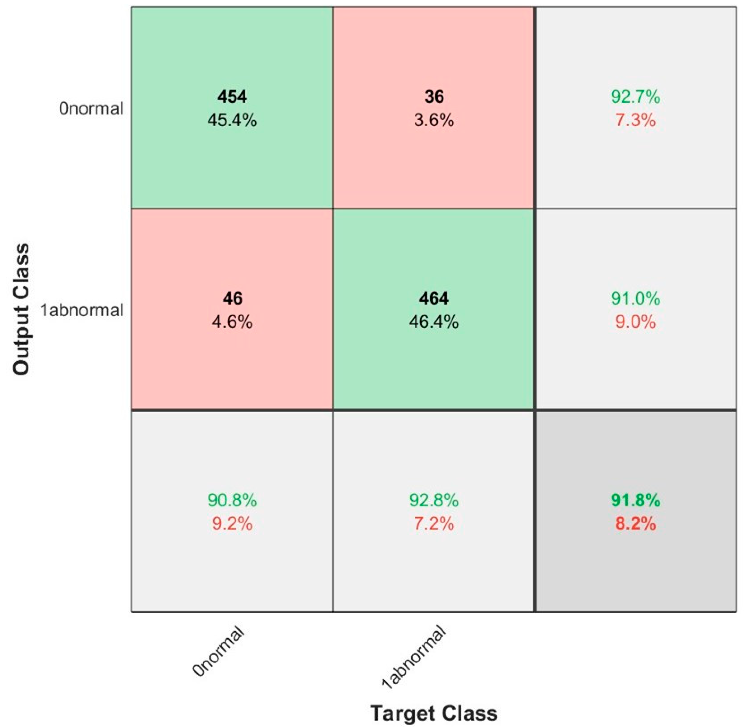
| ResNet-50 | 98.7 | 92.4 | 91.8 | 7329 |
Disclaimer/Publisher’s Note: The statements, opinions and data contained in all publications are solely those of the individual author(s) and contributor(s) and not of MDPI and/or the editor(s). MDPI and/or the editor(s) disclaim responsibility for any injury to people or property resulting from any ideas, methods, instructions or products referred to in the content. |
© 2024 by the authors. Licensee MDPI, Basel, Switzerland. This article is an open access article distributed under the terms and conditions of the Creative Commons Attribution (CC BY) license (https://creativecommons.org/licenses/by/4.0/).
Share and Cite
Senjoba, L.; Ikeda, H.; Toriya, H.; Adachi, T.; Kawamura, Y. Enhancing Interpretability in Drill Bit Wear Analysis through Explainable Artificial Intelligence: A Grad-CAM Approach. Appl. Sci. 2024, 14, 3621. https://0-doi-org.brum.beds.ac.uk/10.3390/app14093621
Senjoba L, Ikeda H, Toriya H, Adachi T, Kawamura Y. Enhancing Interpretability in Drill Bit Wear Analysis through Explainable Artificial Intelligence: A Grad-CAM Approach. Applied Sciences. 2024; 14(9):3621. https://0-doi-org.brum.beds.ac.uk/10.3390/app14093621
Chicago/Turabian StyleSenjoba, Lesego, Hajime Ikeda, Hisatoshi Toriya, Tsuyoshi Adachi, and Youhei Kawamura. 2024. "Enhancing Interpretability in Drill Bit Wear Analysis through Explainable Artificial Intelligence: A Grad-CAM Approach" Applied Sciences 14, no. 9: 3621. https://0-doi-org.brum.beds.ac.uk/10.3390/app14093621