The Impact of the Damping Coefficient on the Dynamic Stability of the TM-AFM Microcantilever Beam System

Abstract

The tapping-mode atomic force microscope (TM-AFM) is widely used today; however, improper matching between the operating medium and the sampling time may lead to inaccurate measurement results. The relationship between the damping coefficient and the steady state of the TM-AFM microcantilever is investigated in this paper using multiple stability theory. Firstly, the effects of changes in dimensionless linear damping coefficients and dimensionless piezoelectric film damping coefficients on the motion stability of the system are examined using bifurcation diagrams, phase trajectories, and domains of attraction. Subsequently, the degrees of effect of the two damping coefficients on the stability of the system are compared. Finally, the bi-parametric bifurcation characteristics of the system under a specific number of iterative cycles are investigated using the bi-parametric bifurcation diagram in conjunction with the actual working conditions, and the boundary conditions for the transition of the system’s motion from an unstable state to a stable state are obtained. The results of the study show that to ensure the accuracy and reliability of the individual measurement data in 500 iteration cycles, the dimensionless linear damping coefficient must be greater than 0.01014. Our results will provide valuable references for TM-AFM measurement media selection, improving TM-AFM imaging quality, measurement accuracy and maneuverability, and TM-AFM troubleshooting.

1. Introduction

Atomic force microscopy (AFM) is widely used to image the surface morphology of polymers, ceramics, glass, and biological cells [1,2,3]. It has three common operation modes: contact, non-contact, and tapping [4,5,6]. The core component of AFM is a microcantilever beam [7]. The tapping mode is preferred for experiments involving biological samples in liquids. The TM-AFM is the most widely used atomic force microscope [8,9,10].

The accuracy of TM-AFM is limited to the angstrom level due to various factors [11,12]. Mathematical modeling can account for these factors as dynamic parameters in the system. The proper matching of dynamic parameters is important to avoid complex dynamics and long steady-state times.

In the past 30 years, researchers have conducted extensive research on the dynamic characteristics of the TM-AFM microcantilever beam system from various perspectives. Based on the JKR (Johnson–Kendall–Roberts) contact model, Berg et al. [13] proposed an interaction model that considers the adhesion effect between the tip and the tested sample. Water et al. [14] analyzed a special mathematical map that exhibits square root singularities, which directly leads to an infinite series period-doubling bifurcation in the system. Roman et al. [15,16] discussed the three-dimensional characteristic modes of both tip and tuning fork tips in TM-AFM microcantilever beams, and summarized their interaction with samples as well as their nonlinear dynamics when moving in liquid environments. Kiracofe et al. [17] measured the vibration of a TM-AFM microcantilever beam in air and water using a scanning laser Doppler vibrometer (Polytec MSA-400 Micro System Analyzer from Polytec Gmbh, Waldbronn, Germany.)

Gmbh, Waldbronn, Germany. Wei Zheng et al. [18,19,20], based on the JKR contact model, provided energy loading and unloading curves under tip–sample interaction conditions to study energy dissipation caused by adhesion, plastic deformation, liquid bridge formation, and air-damping effects. However, the effect of changes in the damping coefficient on the steady-state behavior of the TM-AFM cantilever has not been analyzed from a multiple stability perspective.

The purpose of this paper is to investigate the impact of the damping coefficient on the steady-state behavior of a TM-AFM microcantilever beam through extensive numerical simulations. We also aim to uncover the underlying mechanism by utilizing various stability-related theories and methods. Our objective is to identify the optimal range for the damping coefficient, which is a crucial dynamic parameter during TM-AFM motion. This will serve as a valuable reference for improving imaging quality, measurement accuracy, operability, and troubleshooting potential faults associated with the TM-AFM system.

This paper is organized as follows: Section 2 introduces the mechanical model and motion of the TM-AFM microcantilever beam system. Section 3 analyzes the effect of linear damping coefficients on the motion stability of the system. Section 4 analyzes the effect of the pressure film damping coefficient on the stability of the system and compares it with the effect of the linear damping coefficient. Section 5 analyzes the effect of the coupled action of the dual damping parameters on the stability of the system and determines the boundary conditions for the transition of the system’s motion from an unstable to a stable state. Finally, Section 6 discusses the results and summarizes the whole paper.

2. The Physical Model and Its Dynamic Equations

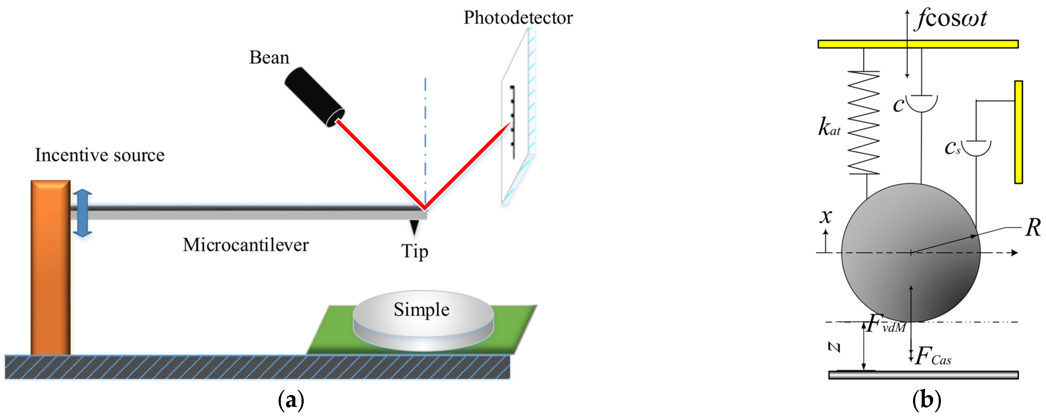
The working principle of TM-AFM is illustrated in Figure 1. The physical model of the microcantilever beam system is commonly represented as a spring-mass-damping system, as depicted in Figure 1b. Meanwhile, its equation of motion can be expressed as [21,22]

$$m\ddot{x}+c_1\dot{x}+c_s\dot{x}+k_{1}x+k_2{x}^3=F_{vdM}(z)+F_{Cas}(z)+f\cos \omega t,$$

(1)

where $x$, $\dot{x}$, and $\ddot{x}$ denote the displacement, velocity, and acceleration of the microcantilever beam in units of m, m/s, and m/s², respectively. During motion, apart from external excitation fcosωt, the microcantilever beam system is also affected by van der Waals force F_vdM, linear spring force, nonlinear spring force (compensating for the linear spring force, equivalent stiffness is expressed in k₂), linear damping force, extruded film damping force (compensating for the linear damping force), and Casimir force F_Cas [21,23,24,25]. z denotes the distance from the tip of the microcantilever beam to the surface of the sample to be measured, assuming that the distance between the tip samples when the microcantilever beam is at rest is l₀, then $z=l_0+x(t)$. To facilitate the study of the dynamic characteristics of the cantilever beam, we introduce dimensionless state space Equation (2) for the cantilever beam system.

$$\left\{\begin{array}{c}\dot{x}=y\\ \dot{y}=-ry-bx-h{x}^3+\frac{e}{{(a+x)}^8}-\frac{d}{{(a+x)}^2}-\frac{p}{{(a+x)}^3}y+\frac{\beta }{{(a+x)}^4}+g\cos (\Omega \tau {)}_{.}\end{array}\right.$$

(2)

The dimensionless displacement and velocity are represented by x and y, respectively. The dimensionless linear damping coefficient is denoted as r, while b and h represent dimensionless linear and nonlinear stiffness, respectively. The strength of the dimensionless Hamaker repulsion potential is represented by e, and the strength of the dimensionless Hamaker attraction potential is represented by d. The dimensionless Casimir force strength is represented by β. The damping coefficient of the extruded film is represented by p in a dimensionless form. The amplitude of external excitation is represented by g in a dimensionless form. The frequency ratio is represented by Ω (Ω = ω/ω_n), where Ω is the external excitation frequency and ω_n is the natural vibration frequency of the microcantilever beam system. The equilibrium distance between the tip of the microcantilever beam and the surface of the measured sample under a static state is represented by a.

Since, in this paper, we mainly study the effect of damping (including equivalent linear damping and extruded air-film damping) on the motion stability of the TM-AFM microcantilever beam system, we only explain the derivation process of the motion parameters r and p here.

In general, the linear damping coefficient c of the spring oscillator can be obtained by the measured method or the finite element integration method, but due to the tiny size of the microcantilever beam, it is difficult to obtain the linear damping coefficient c of the microcantilever beam by the measured method. Therefore, the finite element integration method is used to obtain the linear damping coefficient c of the microcantilever beam of the continuum microcantilever beam of the first-order mode of the formation function as follows [7,18].

$$\phi (y_1)=\cos {\beta }_1-\cosh {\beta }_1{y}_1+r_1(\sin {\beta }_1{y}_1-\sinh {\beta }_1{y}_1),$$

(3)

where $y_1$ denotes the distance from the reference point on the axial beam to the fixed end of the left end of the microcantilever beam, y_1max = l, l denotes the length of the microcantilever beam, ${\beta }_1=\frac{\pi }{l}$, $r_1=\frac{\sin {\beta }_{1}l-\sinh {\beta }_{1}l}{\cos {\beta }_{1}l+\cosh {\beta }_{1}l}$. Let the relative displacement of the microcantilever beam concerning the base at the left end be x₁($y_1$,t), the damping coefficient per unit length of the microcantilever beam be $c_0$, and the energy dissipated by the simplified spring oscillator in one cycle of motion be equal to the energy loss in one cycle of motion of the continuum microcantilever beam, i.e.,

$${\displaystyle {\int }_0^l{\displaystyle {\int }_{-\phi (y_1)E}^{\phi (y_1)E}{c}_0\frac{\partial x_1(y_1,t)}{\partial t}}}d{x}_{1}d{y}_1={\displaystyle {\int }_{-\phi (l)E}^{\phi (l)E}{c}_1\frac{\partial x_1(l,t)}{\partial t}}d{x}_1,$$

(4)

the equivalent linear damping of the spring oscillator can be found to be

$$c=\frac{c_{0}l}{{\phi }^2(l)}.$$

(5)

The relationship between the quality factor of the spring-loaded vibrator system and the equivalent linear damping is given by

$$Q=\frac{m{\omega }_n}{c},$$

(6)

after the dimensionless process, the dimensionless linear damping coefficient is

$$r=\frac{1}{Q}.$$

(7)

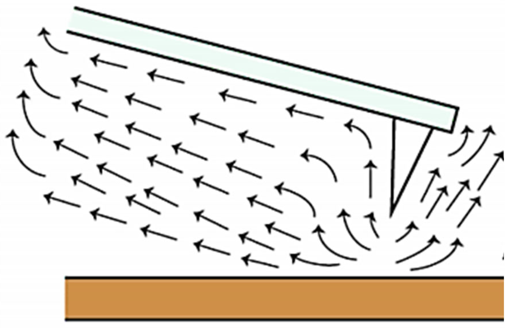
When the tip of the microcantilever beam is close to the surface of the sample to be measured, the vibration of the tip leads to the existence of radial and axial relative motion between the tip and the sample to be measured, x₂ and y₂; it is necessary to take into account the tip and the sample to be measured between the extrusion of the gas film on the microcantilever beam system of the damping force. The microcantilever beam tip is equivalent to the spherical surface; at this time, it is assumed that only the microcantilever beam tip is subjected to the extrusion of the film force, and the rest of the microcantilever beam of the medium is regarded as an ideal fluid, as shown in Figure 2.

The squeezing number τ_c determines the compressibility of the air film, which in the TM-AFM microcantilever beam system can be expressed as [26]

$${\tau }_c=\frac{12{\mu }_{eff}\omega l_s^2}{P_a{z}^2},$$

(8)

where μ_eff is the effective medium gas viscosity coefficient, l_s is defined as the characteristic length of the moving object in the flow field, where the characteristic length l_s is approximately equal to the diameter of the tip-equivalent sphere, P_a is the ambient pressure, and P_a is related to the kinetic viscosity η and the Knudsen number k_n as follows [27]:

$${\mu }_{eff}=\frac{\eta }{1+9.638k_n^{1.159}},$$

(9)

and the squeezing membrane force on the tip needs to satisfy the nonlinear Reynolds equation [28]:

$$\frac{\partial }{\partial y_2}(z^{3}P\frac{\partial P}{\partial y_2})+\frac{\partial }{\partial x_2}(z^{3}P\frac{\partial P}{\partial x_2})=12{\mu }_{eff}\frac{\partial (P z)}{\partial t},$$

(10)

P is the pressure distribution on the tip surface, P = P_a + ΔP, and ΔP is the bias pressure caused by squeezing the air film.

The pressure gradient upward of the negligible cantilever beam, Equation (10) can be simplified to obtain

$$\frac{{\partial }^{2}P}{\partial x_2^2}=\frac{12{\mu }_{eff}}{z^3}\frac{\partial z}{\partial t}$$

(11)

Integrate Equation (11) in the direction of the radius of the sphere and introduce the boundary conditions: x = ±R, P = P_a; x = 0. This yields the bias pressure caused by squeezing the gas film ΔP

$$\Delta P=-\frac{6{\mu }_{eff}}{z^3}(R^2-z^2)\frac{dz}{dt}.$$

(12)

Then, integrating Equation (12) along the sphere yields the resistance of the extruded air film at the tip of the microcantilever beam as

$$F_s={\displaystyle {\int }_0^{2R}{\displaystyle {\int }_{-R}^R\Delta Pd{x}_{2}d{y}_2}}=-\frac{16R^4{\mu }_{eff}}{z^3}\frac{dz}{dt},$$

(13)

which yields the equivalent extruded membrane damping coefficient

$$c_s=\frac{16R^4{\mu }_{eff}}{z^3}.$$

(14)

In the dimensionless process, the equilibrium distance parameters $l_b=(3/2){(2D)}^{1/3}$, $D=BR/(6k_1)$, B is defined to denote the Hamaker attraction potential constants, and finally, we obtain the dimensionless extruded film damping coefficient

$$p=\frac{16{\mu }_{eff}{R}^7}{m{\omega }_n{l}_b^3}.$$

(15)

The dynamic parameters of the system are fixed as follows: a = 1.6, b = 0.05, h = 0.35, d = 0.1481, e = 0.0001, β = 0.002, g = 0.2, Ω = 1. In the following work, except for the change of parameters r and p, the other parameters in Equation (2) remain unchanged. Please note that the detailed derivation process of the dimensionless state-space equation and the selection process of parameters are shown in references [21,22]. To avoid repetition, they are not repeated here.

3. Effect of Linear Damping on System Stability

From the analysis in Section 1, we know that the TM-AFM microcantilever beam system is affected by both linear damping force and squeeze film damping force during motion. To analyze in detail the degree of effect of the two kinds of damping forces on the motion stability of the system, in Section 3 and Section 4, we temporarily weaken the physical properties of the system to discuss its mathematical properties, and adopt fixing one kind of damping force and varying the other to discuss the two kinds of forces separately, and in this section, we make p = 0.006.

3.1. No Dimensional Damping Coefficient Changes

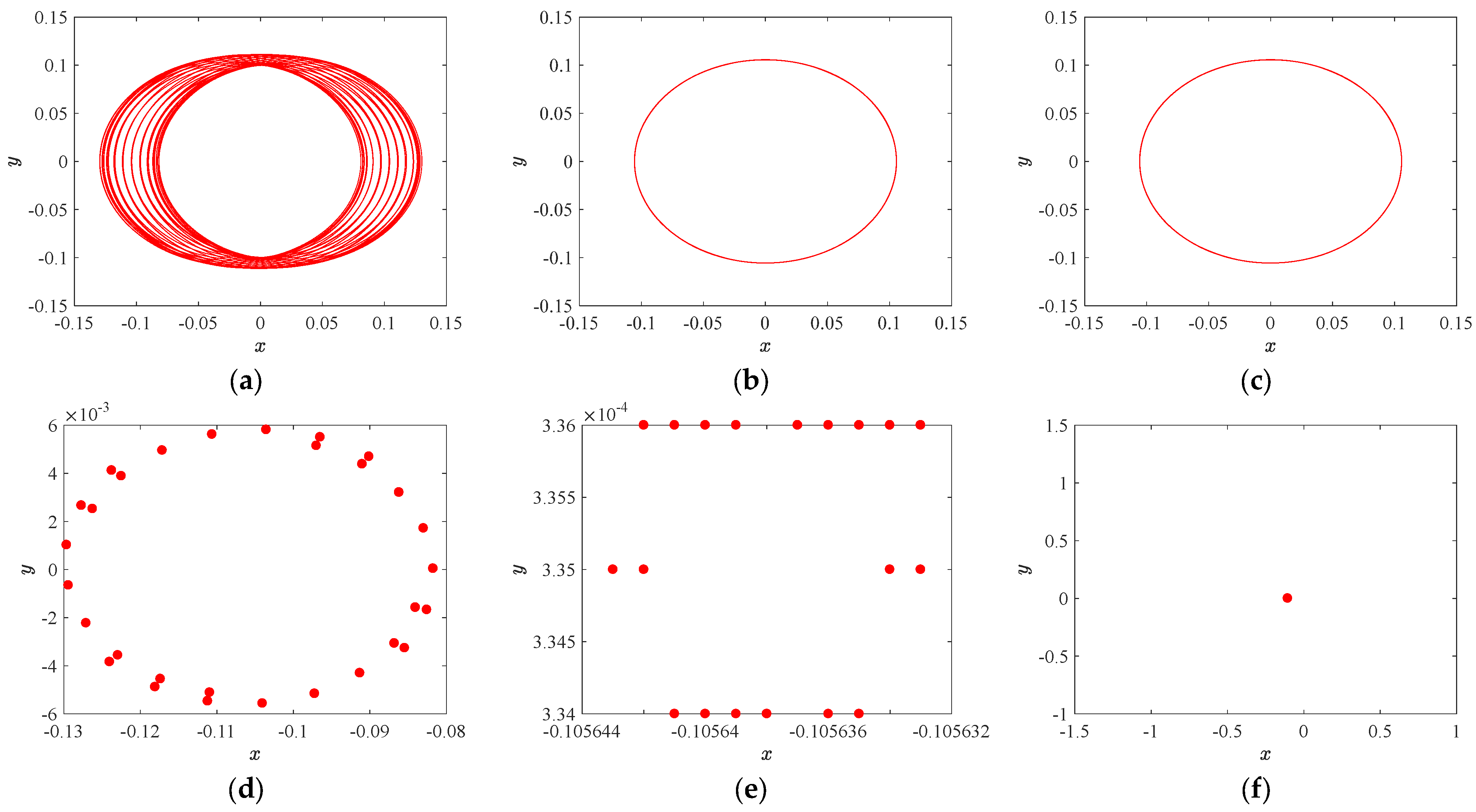
Equation (2) is an iterative equation. We introduce the concept of the number of iteration cycles M here, which represents the time it takes for the system to transition from a resting state to an investigative state. When given that M = 500 iteration cycles and the initial values (x₀, y₀) = (0, 0), with r equal to 0.001, 0.003, and 0.005, respectively, Figure 2 shows the phase trajectory diagrams and Poincaré cross-sections of system (2).

After analyzing Figure 3, it can be observed that for a given cycle number M = 500, the motion stability of system (2) gradually increases with an increase in the damping coefficient. It is worth noting that even though the error during the cycle in the phase trajectory diagram of system (2) is already tiny when r equals 0.003, which cannot be identified solely based on the phase trajectory diagram and requires reliance on the Poincaré cross-section, for micro- and nano-measurements using TM-AFM, this tiny error will be amplified by the optical lever principle and detected by the photoelectric displacement sensor, resulting in increased measurement errors.

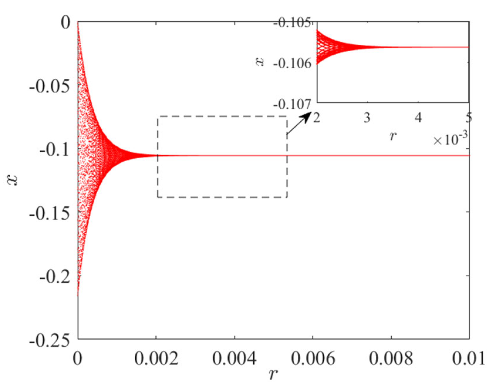
To further analyze the evolution law of system (2)’s stability as the damping coefficient changes, with r being taken as the independent variable, Figure 4 shows the bifurcation diagram of system (2) when r ∈ (0, 0.01).

It can also be observed from Figure 4 that as r gradually increases, the number of bifurcations in the bifurcation diagram decreases gradually and consequently enhances the motion stability of system (2).

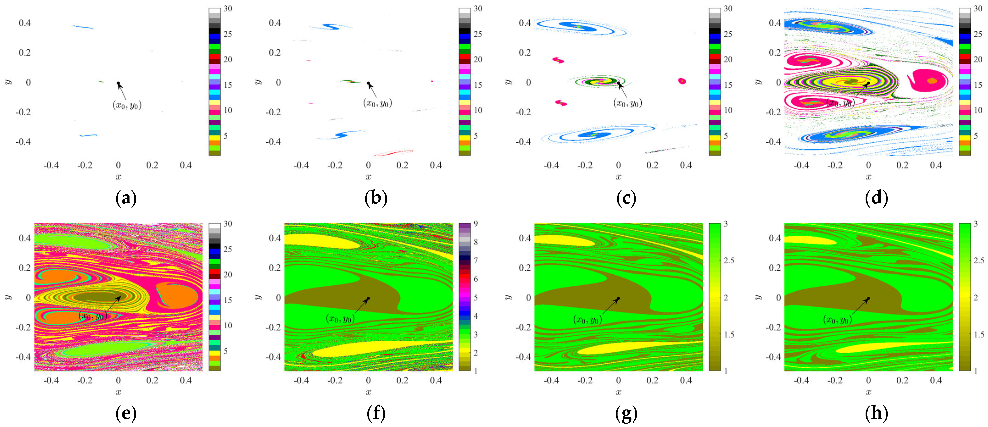
The iterative cycle is repeated 500 times, with the initial value point set as (x₀, y₀) = (0.0), r ranging from 0.001 to 0.008 with a step size of 0.001. The attractive domains of system (2) in the x ∈ (−0.5, 0.5), y ∈ (−0.5, 0.5) space as shown in Figure 5.

When r = 0.005, although the initial value point is located in the suction basin of period 1 as shown in Figure 5e, the space occupied by the suction basin of period 1 is not large, and there are several ribbon-like quasi-periodic suction basins outside the suction basin of period 1; therefore, system (2) has relatively poor anti-interference ability. Additionally, considering that the variation in r between Figure 5a–h is 0.001, there is a very fast evolution speed of the attraction domain in space from Figure 5a–e, resulting in obvious changes in the image of the attraction domain; however, from Figure 5f–h, there is a slow evolution speed for the attraction domain in space and almost no change in shape or area for the central part of the attraction basin during period 1. The speed at which the suction basin nears its initial value point evolves and can also be used to evaluate system stability: faster evolution indicates a higher likelihood for changes in where this initial value point lies within its corresponding suction basin and thus suggests an unstable motion state for this system; conversely, slower evolution rates indicate greater stability for both their respective suction basins and the corresponding system motion states.

3.2. The Number of Iteration Cycles Changes

The analysis results in Section 3.1 are obtained on the premise that the number of iteration cycles is fixed; that is, the long-term properties of the motion characteristics of system (2) are not considered. However, the long-term nature and behavior of a motor system are important components of system stability. It is meaningless to discuss the stability of the system without considering the time scale. In this section, we will analyze the number of iterative cycles, that is, the relationship between the motion time and the motion stability of system (2), in combination with the conclusion of the motion stability of system (2) above.

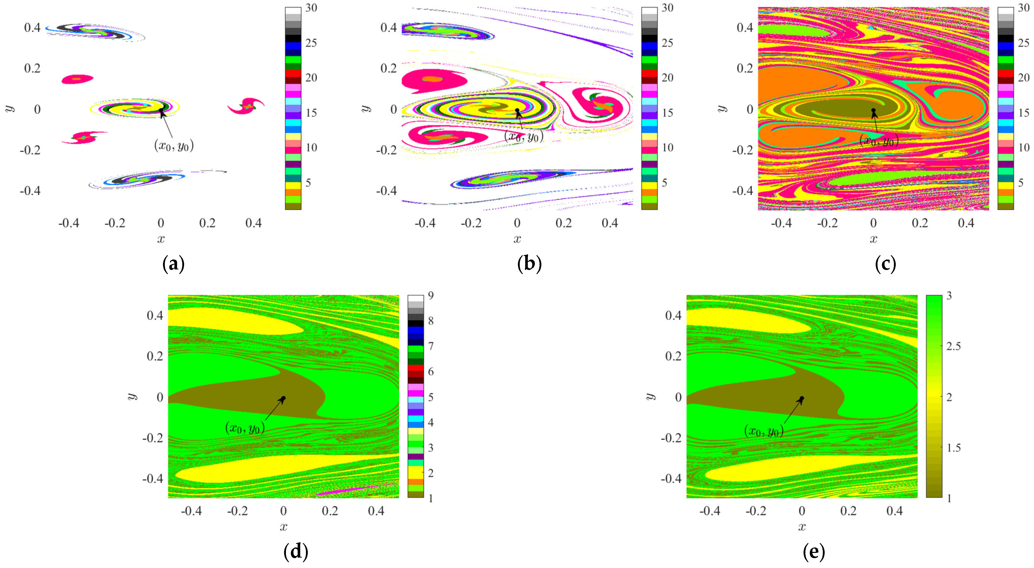
When the number of iteration cycles is 300 and r takes values of 0.006, 0.007, and 0.009, respectively, the attraction domains are shown in Figure 6a–c. When the number of iteration cycles is 1000 and r is equal to 0.003 and 0.004, respectively, the attraction domains are shown in Figure 6d,e.

The number of iteration cycles has a direct relationship with the motion stability of system (2), as shown in Figure 6; the more iteration cycles, the closer system (2) is to a stable state; conversely, the fewer the number of iteration cycles, the worse the stability of system (2).

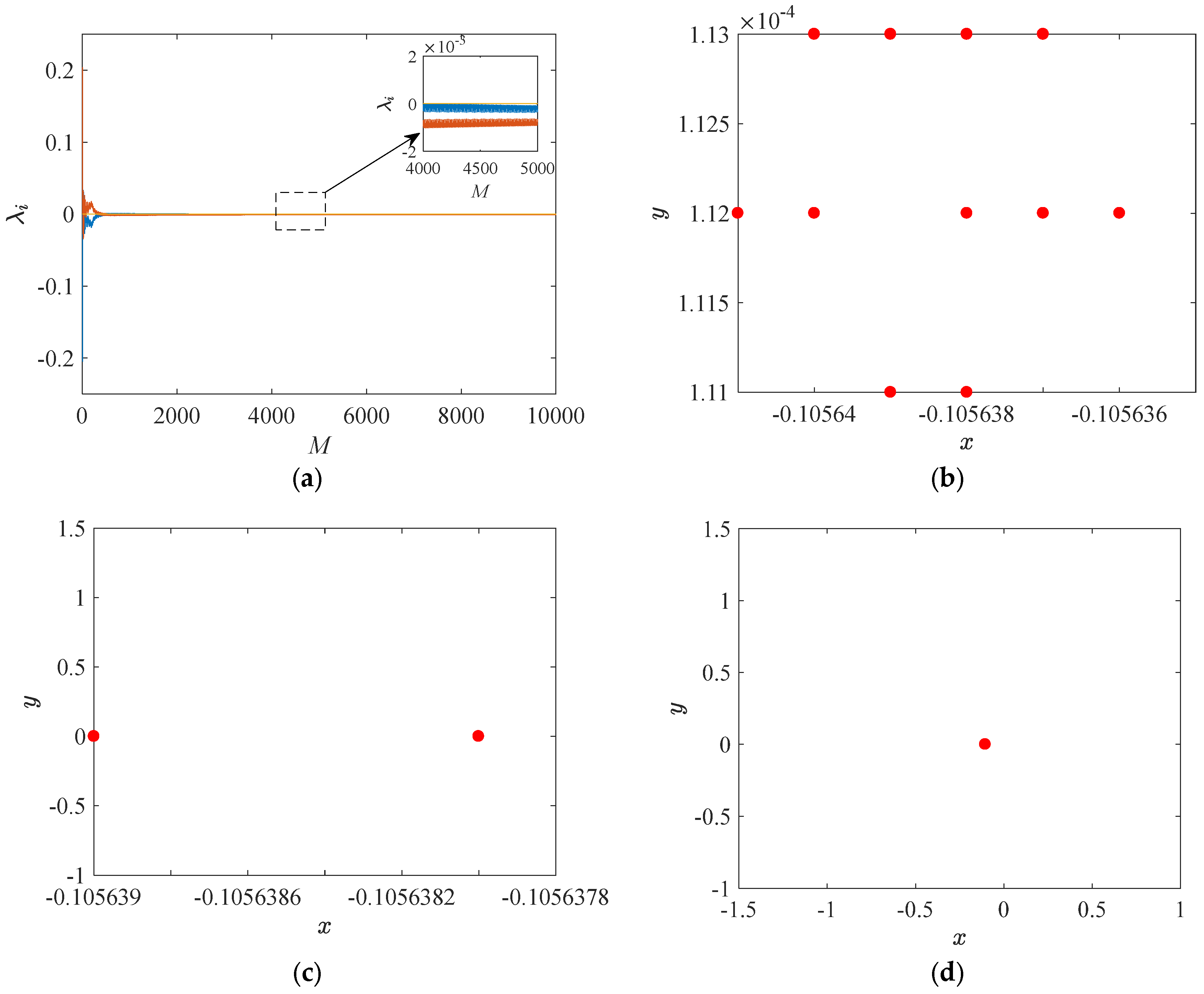
According to Figure 5, as system (2) approaches a stable state, the rate of evolution in its attraction region slows down; whereas according to Lyapunov stability correlation theory, under certain parameter conditions, the smaller the Lyapunov exponents of system (2), the more stable it becomes. By referring to the M-Lyapunov exponents diagram and Poincaré cross-section, we can determine the number of iteration cycles required for system (2) to reach a steady state given these parameter conditions.

Figure 5 has already shown that when M ≥ 500 and r ≥ 0.006, system (2) is in a stable state. Now, let us take r = 0.001 as an example to determine the number of iteration cycles M required for system (2) to become stable, as shown in Figure 7.

Based on the analysis in this chapter, we conclude that when fixing p = 0.006, a low linear damping coefficient will result in the system taking longer to reach stability, while a high linear damping coefficient allows the system to enter the steady state relatively faster.

4. Effect of Extrusion Film Damping on System Stability

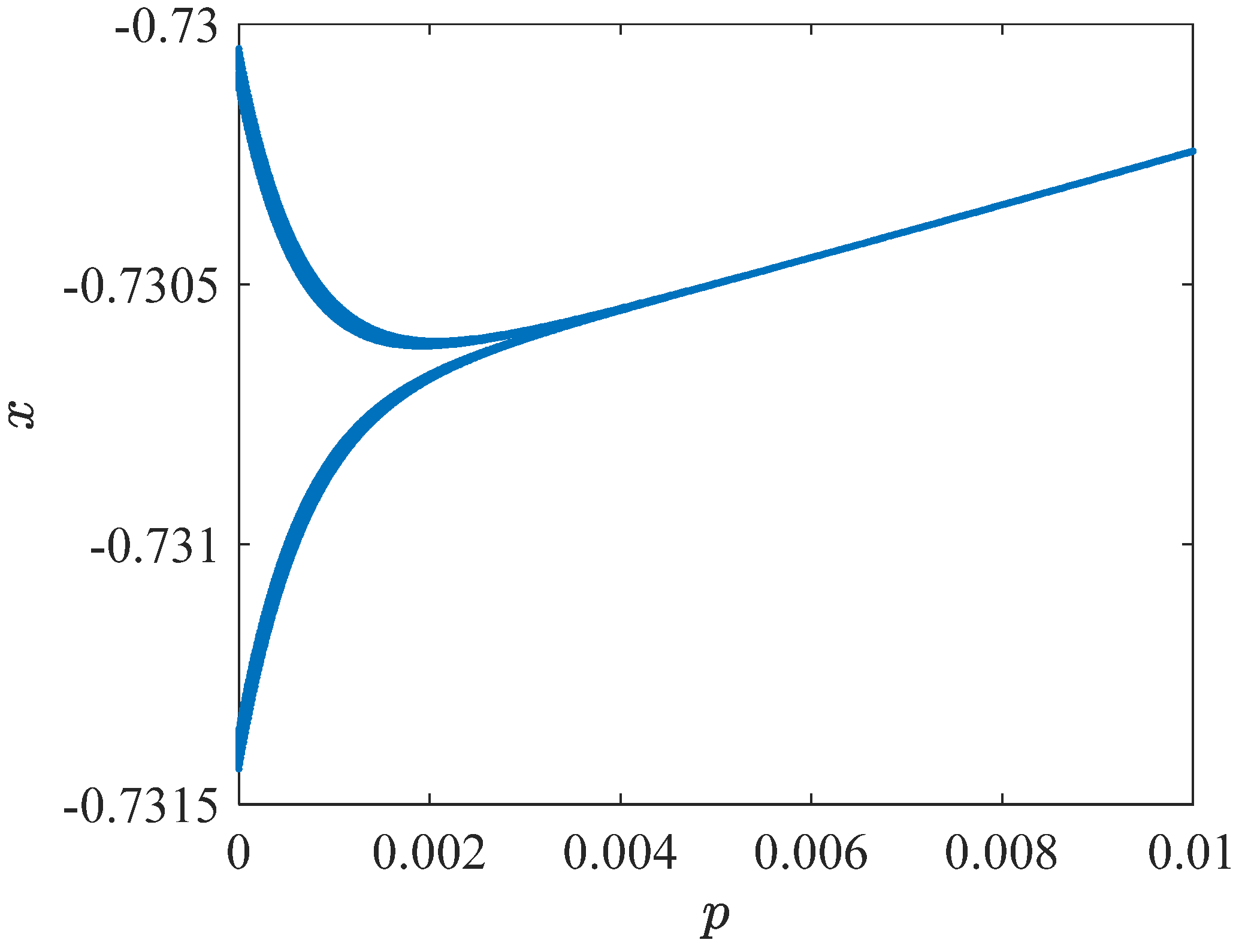
In Section 3, we found that system (2) reaches a steady state when p = 0.006, M = 500, and r ≥ 0.006. In this section, we fix the linear damping coefficient r = 0.008 and analyze its effect on the motion stability of system (2) by varying the dimensionless piezoelectric membrane damping coefficient p. Figure 8 shows the bifurcation diagram of system (2) when p ∈ (0, 0.01).

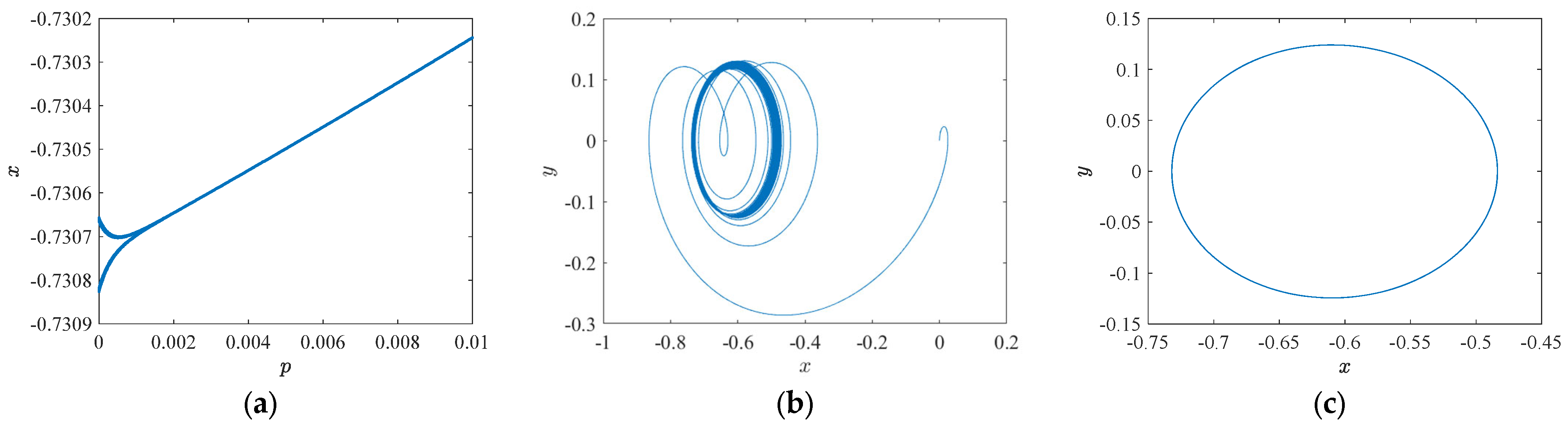
Comparing Figure 4 and Figure 8, Figure 8 seems to contain a ring surface time-period bifurcation, and the appearance of such bifurcation characteristics is often accompanied by a change in the system kinematic characteristics, i.e., the squeezed membrane damping force may affect not only the stability of the system but also the kinematic characteristics of system (2). To further determine the type of bifurcation, the number of iterative cycles M was increased to 1000, and the phase trajectories of system (2) are plotted when M is equal to 500 and 1000, respectively, and p = 0.001 to analyze whether the dimensionless squeezed membrane damping coefficient p affects the dynamics of the system, as shown in Figure 9.

Comparing Figure 8 and Figure 9a, it can be seen that when the number of iterative loops is increased, the “multiplicative bifurcation point” is shifted to the left significantly, and it is obvious that if the parameter p affects the dynamics of the system, the position of the “multiplicative bifurcation point” will not be affected by the number of iterative loops. Therefore, the cyclic surface multiplicative bifurcation is not included in Figure 8. By comparing Figure 9b and Figure 9c, the above conclusion can also be confirmed.

In summary, piezo membrane damping, like equivalent linear damping, does not affect the final dynamics of system (2), and the low piezo membrane damping coefficients will likewise result in the system taking longer to stabilize.

Furthermore, in Figure 4’s bifurcation diagram, the maximum span of the vertical coordinate is 0.215, while in Figure 8, the maximum span of the vertical coordinate is 0.00138, i.e., the maximum span of the longitudinal coordinate in Figure 4 is 155.8 times the maximum span of the longitudinal coordinate in Figure 8, which is the same conclusion as that obtained by the energy dissipation method. That is, we prove the corresponding conclusion of the energy dissipation theory with the multiple stability theory.

5. Effect of the Coupled Action of Double Damping Parameters on the Stability of the System

The analytical process in Section 3 and Section 4 weakens the physical properties of damping, but in real working conditions, the equivalent linear damping and pressure film damping are coupled with each other, i.e., the change of one parameter is accompanied by the change of the other parameter, so in this section, we analyze the effect of the coupling effect of the dual damping parameters on the stability of the system.

By associating Equations (6), (7) and (15) and introducing dimensionless quantities, the relationship between the dimensionless linear damping coefficient r and the dimensionless piezoelectric membrane damping coefficient p is obtained as

$$p=r·\frac{16{\mu }_{eff}{R}^7}{l_b^3},$$

(16)

and from Equation (16), r is positively correlated with p. Under the premise that the material and structure of the microcantilever beam are fixed, R and l_b are constant, but when r is changed, i.e., the medium changes, the effective medium gas–viscosity coefficient μ_eff will likewise change, so r is nonlinearly related to p. Combining the relevant experimental data in references [21,22], we introduce here the quadratic nonlinear fitting relationship curves L₁ and L₂ for p and r,

$$L_1:p=-0.98r^2+0.198r,L_2:p=0.79r^2+0.022r.$$

(17)

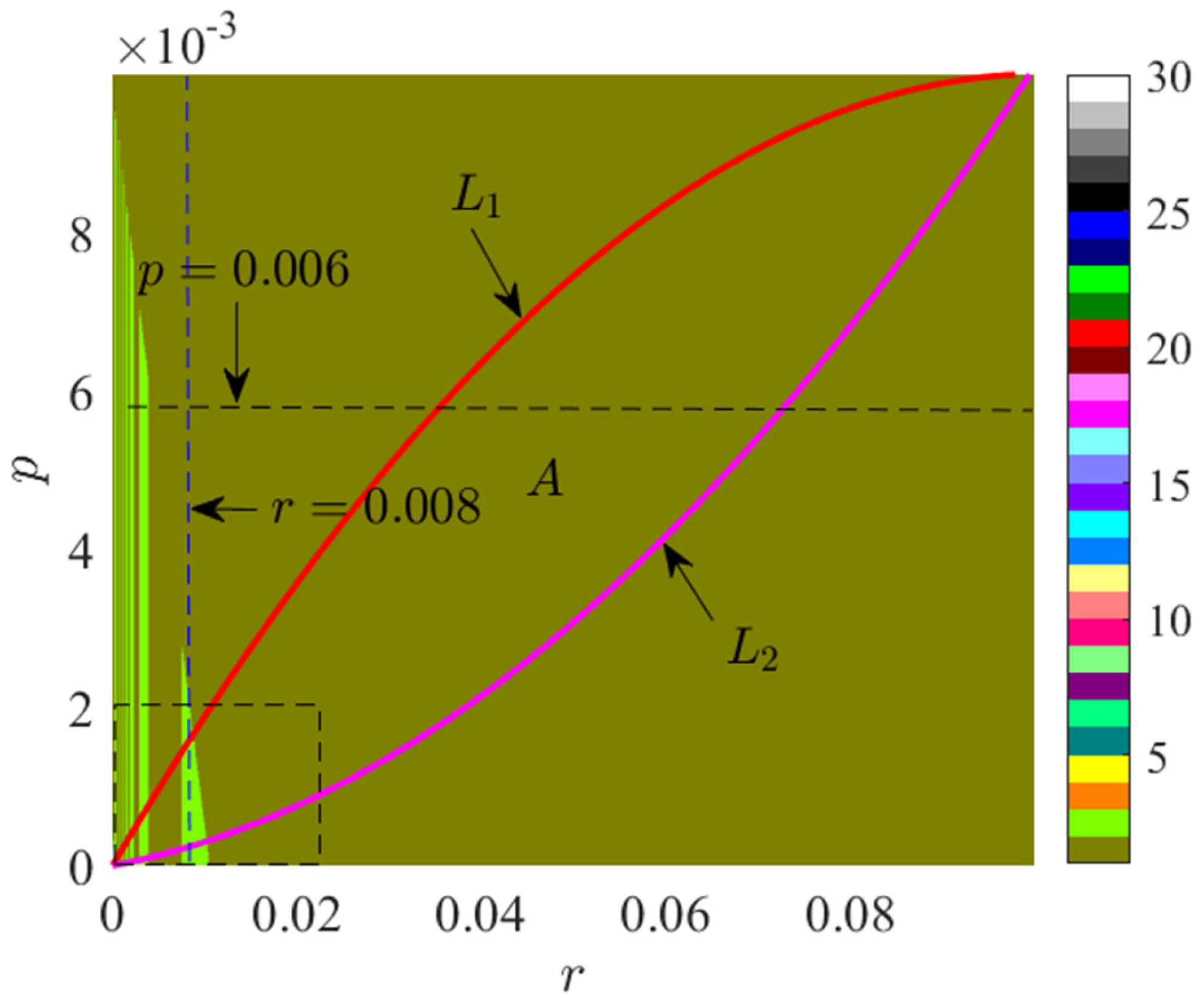
The two-parameter bifurcation diagram in the parameter plane of system (2) r × p when r ∈ (0, 0.1), p ∈ (0, 0.01), and the number of iterative cycles M = 500 is shown in Figure 10.

In Figure 10, the black dashed line p = 0.006 is equivalent to Figure 4, and the blue dashed line r = 0.008 is equivalent to Figure 8. Meanwhile, we add the fitting curves L₁ and L₂ as auxiliary lines in Figure 10. It is worth noting that the magnitude of the effective medium gas–viscosity coefficient μ_eff is not only related to the medium, but the air pressure and temperature also make it change, and at the same time, due to the coupling relationship between the dimensionless linear damping coefficient r and the dimensionless piezoelectric film damping coefficient p, in Figure 10, system (2) has real physical significance only in the region wrapped by L₁ and L₂, while region A has actual physical significance.

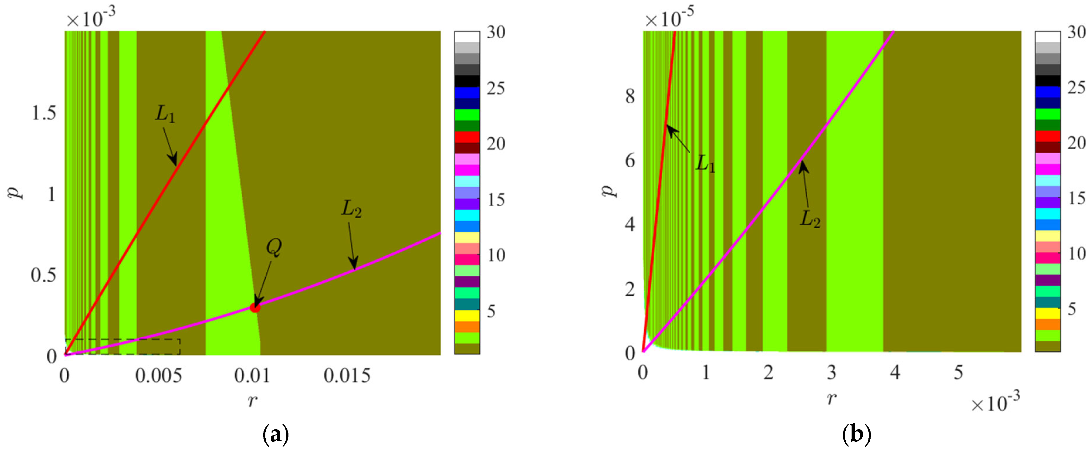
To further analyze the coupling relationship between r and p, and to find the boundary conditions for system (2) to reach a steady state of motion under the condition of a fixed number of iterative loops, Figure 10 is locally enlarged (the part of the black dashed box in Figure 10), i.e., we obtain the two-parameter bifurcation diagram of system (2) in the r × p parameter plane at r ∈ (0, 0.02), and p ∈ (0, 0.002), which is shown in Figure 11a.

In Figure 11a, we can see the bifurcation characteristics of system (2) in the r × p parameter plane, and at the same time, we obtain the boundary conditions for the transition of the motion state of system (2) from an unstable to a stable state under the condition of M = 500, i.e., the intersection point Q of the period 2 region in the positive direction and L₂, at which time, the coordinate of the point Q is (r, p) = (0.01014, 0.00031).

In addition, Figure 11a is further enlarged to obtain the two-parameter bifurcation diagram of system (2) in the r × p parameter plane for r ∈ (0, 0.006) and p ∈ (0, 0.0001) as shown in Figure 11b, and in Figure 11b, we can observe that there are obvious hierarchical, branching repetitive, and scaling properties in the two-parameter inverse bifurcation diagram. At the same time, we can observe the trajectories of the system evolving from an unstable to a stable state, and observing these trajectories, can help us to understand how system (2) searches for stability in the parameter space.

6. Discussion and Conclusions

Combined with the physical significance of system (2), the first-order resonant angular frequency of a microcantilever beam is usually (1000~20,000) Hz, and the corresponding vibration period is (0.0003~0.0060) s, which depends on whether or not there is a coating or using the coating material that is not used. According to the analysis in Section 3, we know that when p = 0.006, the motion state of system (2) can be stabilized in (0.15~3) s (M = 500) if r = 0.006; if r = 0.001, it takes (1.5~30) s (M = 5000) to be stabilized. When measuring the surface shape of an object under test, the TM-AFM needs to measure thousands of feature points. However, if measuring each feature point requires several seconds or even tens of seconds of stabilization time to ensure accurate and reliable measurement data, such inefficiency may not meet the requirements of practical working conditions.

Finally, we can conclude the following by combining the coupling nature of the double damping parameters under the actual working conditions and the found boundary conditions that to ensure the accuracy and reliability of the single measurement data in 500 iteration cycles, the value of the dimensionless linear damping coefficient r must be greater than 0.01014.

The paper studies the effect of the damping coefficient on the motion characteristics of the TM-AFM microcantilever beam system using multiple stability theory. By keeping the number of iteration periods constant and varying the dimensionless linear damping coefficient and the dimensionless piezoelectric membrane damping coefficient, we found that increasing the dimensionless linear damping coefficient or increasing the dimensionless piezoelectric membrane damping coefficient can shorten the time required for the system to transition from an unsteady to a stable state under the given parameter conditions. In addition, we obtained the boundary conditions for the transition of the system from the unstable state to the stable state by using the bifurcation diagram of the dual damping parameter coupling. Finally, after considering the actual operating conditions of the TM-AFM, we conclude that the dimensionless damping coefficient of the operating medium of the TM-AFM microcantilever beam must be greater than 0.01014 to ensure the accuracy and reliability of the measured data in 500 iteration cycles. The research findings presented in this paper provide valuable references for media selection in TM-AFM measurements, enhancing imaging quality, measurement accuracy, and troubleshooting.

Based on Equation (2), it is evident that there are numerous dynamic parameters present in system (2). The multiple stability theory discussed in this paper can be effectively used to analyze the impact of these dynamic parameters on the distinctive properties of system motion. In the future, we intend to conduct additional research to explore these topics in greater detail.

References

- Zhang, Z.; Smith, K.; Jervis, R.; Shearing, P.R.; Miller, T.S.; Brett, D.J.L. Operando Electrochemical Atomic Force Microscopy of Solid–Electrolyte Interphase Formation on Graphite Anodes: The Evolution of SEI Morphology and Mechanical Properties. ACS Appl. Mater. Interfaces 2020, 12, 35132–35141. [Google Scholar] [CrossRef] [PubMed]
- Bhadauriya, S.; Zhang, J.; Lee, J.; Bockstaller, M.R.; Karim, A.; Sheridan, R.J.; Stafford, C.M. Nanoscale Pattern Decay Monitored Line by Line via In Situ Heated Atomic Force Microscopy. ACS Appl. Mater. Interfaces 2020, 12, 15943–15950. [Google Scholar] [CrossRef] [PubMed]
- Scheuring, S.; Jiang, Y.; Wang, Z.; Miyagi, A. High-Speed Atomic Force Microscopy for Dynamic Single Molecule Structural Biology. Biophys. J. 2023, 122, 2A. [Google Scholar] [CrossRef]
- Abbasi Moud, A. Cellulose Nanocrystals Examined by Atomic Force Microscopy: Applications and Fundamentals. ACS Food Sci. Technol. 2022, 2, 1789–1818. [Google Scholar] [CrossRef]
- Chen, Z.; Chen, F.; Wang, D.; Zhou, L. Tapping Modes in the Atomic Force Microscope Model with Lennard-Jones Force and Slow-Fast Base Motion. Chaos Solitons Fractals 2021, 144, 110696. [Google Scholar] [CrossRef]
- Bahrami, M.R. Dynamic Analysis of Atomic Force Microscope in Tapping Mode. Vib. Proced. 2020, 32, 13–19. [Google Scholar] [CrossRef]
- Wang, Y.D. Research on the Technique and System of High Speed Atomic Force Microscope. Ph.D. Thesis, Zhejiang University, Hangzhou, China, 2021. (In Chinese). [Google Scholar]
- Dzedzickis, A.; Bučinskas, V.; Lenkutis, T.; Morkvėnaitė-Vilkončienė, I.; Kovalevskyi, V. Increasing Imaging Speed and Accuracy in Contact Mode AFM. In Automation 2019; Szewczyk, R., Zieliński, C., Kaliczyńska, M., Eds.; Advances in Intelligent Systems and Computing; Springer International Publishing: Cham, Switzerland, 2020; Volume 920, pp. 599–607. ISBN 978-3-030-13272-9. [Google Scholar]
- Li, C.; Ostadhassan, M.; Guo, S.; Gentzis, T.; Kong, L. Application of PeakForce Tapping Mode of Atomic Force Microscope to Characterize Nanomechanical Properties of Organic Matter of the Bakken Shale. Fuel 2018, 233, 894–910. [Google Scholar] [CrossRef]
- Smirnov, A.; Yasinskii, V.M.; Filimonenko, D.S.; Rostova, E.; Dietler, G.; Sekatskii, S.K. True Tapping Mode Scanning Near-Field Optical Microscopy with Bent Glass Fiber Probes. Scanning 2018, 2018, 3249189. [Google Scholar] [CrossRef]
- Pasha, A.H.G.; Sadeghi, A. Experimental and Theoretical Investigations about the Nonlinear Vibrations of Rectangular Atomic Force Microscope Cantilevers Immersed in Different Liquids. Arch. Appl. Mech. 2020, 90, 1893–1917. [Google Scholar] [CrossRef]
- Naitoh, Y.; Li, Y.J.; Sugawara, Y. Atomic-Scale Elastic Property Probed by Atomic Force Microscopy. In Comprehensive Nanoscience and Nanotechnology; Elsevier: Amsterdam, The Netherlands, 2019; pp. 33–52. ISBN 978-0-12-812296-9. [Google Scholar]
- Berg, J.; Briggs, G.A.D. Nonlinear Dynamics of Intermittent-Contact Mode Atomic Force Microscopy. Phys. Rev. B 1997, 55, 14899–14908. [Google Scholar] [CrossRef]
- Water, W.V.D.; Molenaar, J. Dynamics of Vibrating Atomic Force Microscopy. Nanotechnology 2000, 11, 192–199. [Google Scholar] [CrossRef]
- Raman, A.; Melcher, J.; Tung, R. Cantilever Dynamics in Atomic Force Microscopy. Nano Today 2008, 3, 20–27. [Google Scholar] [CrossRef]
- Raman, A.; Reifenberger, R.; Melcher, J.; Tung, R. Cantilever Dynamics and Nonlinear Effects in Atomic Force Microscopy. In Noncontact Atomic Force Microscopy; Morita, S., Giessibl, F.J., Wiesendanger, R., Eds.; NanoScience and Technology; Springer: Berlin/Heidelberg, Germany, 2009; pp. 361–395. ISBN 978-3-642-01494-9. [Google Scholar]
- Kiracofe, D.; Raman, A. On Eigenmodes, Stiffness, and Sensitivity of Atomic Force Microscope Cantilevers in Air versus Liquids. J. Appl. Phys. 2010, 107, 033506. [Google Scholar] [CrossRef]
- Wei, Z.; Sun, Y.; Wang, Z.R.; Wang, K.J.; Xu, X.H. Energy Dissipation in Tapping Mode Atomic Force Microscopy. Chin. J. Theor. Appl. Mech. 2017, 49, 1301–1311. (In Chinese) [Google Scholar]
- Liu, G.L.; Zeng, Y.; Liu, J.H.; Wei, Z. Study on Energy Dissipation in the Dynamic System of Tapping Mode Atomic Force Microscope. Chin. J. Theor. Appl. Mech. 2023, 55, 2599–2613. (In Chinese) [Google Scholar]
- Liu, Y.H.; Zheng, X.T.; Wei, Z. Research on the Characteristics of Phase and Frequency Shift in the Tapping Mode of Atomic Force Microscopy. Mach. Des. Manuf. Eng. 2020, 49, 97–100. (In Chinese) [Google Scholar]
- Ribeiro, M.A.; Balthazar, J.M.; Lenz, W.B.; Rocha, R.T.; Tusset, A.M. Numerical Exploratory Analysis of Dynamics and Control of an Atomic Force Microscopy in Tapping Mode with Fractional Order. Shock Vib. 2020, 2020, 4048307. [Google Scholar] [CrossRef]
- Song, P.; Li, X.; Cui, J.; Chen, K.; Chu, Y. Investigation on the Impact of Excitation Amplitude on AFM-TM Microcantilever Beam System’s Dynamic Characteristics and Implementation of an Equivalent Circuit. Sensors 2023, 24, 107. [Google Scholar] [CrossRef] [PubMed]
- Rodrigues, K.D.S.; Balthazar, J.M.; Tusset, A.M.; De Pontes, B.R.; Bueno, Á.M. Preventing Chaotic Motion in Tapping-Mode Atomic Force Microscope. J. Control Autom. Electr. Syst. 2014, 25, 732–740. [Google Scholar] [CrossRef]
- Hsieh, C.-T.; Yau, H.-T.; Wang, C.-C.; Hsieh, Y.-S. Nonlinear Behavior Analysis and Control of the Atomic Force Microscope and Circuit Implementation. J. Low Freq. Noise Vib. Act. Control. 2019, 38, 1576–1593. [Google Scholar] [CrossRef]
- Balthazar, J.M.; Tusset, A.M.; De Souza, S.L.T.; Bueno, A.M. Microcantilever Chaotic Motion Suppression in Tapping Mode Atomic Force Microscope. Proc. Inst. Mech. Eng. Part C J. Mech. Eng. Sci. 2013, 227, 1730–1741. [Google Scholar] [CrossRef]
- Kong, X.; Deng, J.; Dong, J.; Cohen, P.H. Study of Tip Wear for AFM-Based Vibration-Assisted Nanomachining Process. J. Manuf. Process. 2020, 50, 47–56. [Google Scholar] [CrossRef]
- Altuğ Bıçak, M.M.; Rao, M.D. Analytical Modeling of Squeeze Film Damping for Rectangular Elastic Plates Using Green’s Functions. J. Sound Vib. 2010, 329, 4617–4633. [Google Scholar] [CrossRef]
- Bao, M.; Yang, H. Squeeze Film Air Damping in MEMS. Sens. Actuators A Phys. 2007, 136, 3–27. [Google Scholar] [CrossRef]
Figure 1.
The schematic diagrams of the TM-AFM: (a) microcantilever schematic diagram; (b) physical model of the tip represented by a mass-spring-damper system.
Figure 2.
Schematic representation of the effect of extruded air film on the fluid in the vicinity of a micro cantilever beam system.
Figure 3.
Phase trajectories and Poincaré cross sections of system (2) with different r values: (a,d) r = 0.001, system (2) exhibits an extremely unstable state of motion; (b,e) r = 0.003, system (2) shows a motion state of period 19, and its stability is improved; (c,f) r = 0.005, the motion state of system (2) is stable and the motion is period 1.
Figure 4.
r ∈ (0, 0.01), bifurcation diagram of system (2).
Figure 5.
When r is different, the attraction domains of system (2) in the space x ∈ (−0.5, 0.5), y ∈ (−0.5, 0.5): (a–d) exhibit unstable motion states; while (e–h) demonstrate relatively stable motion states.
Figure 6.
The attraction domains of system (2) in the space x ∈ (−0.5, 0.5), y ∈ (−0.5, 0.5): (a–c) when M = 300, the system that was stable at M = 500 becomes unstable; (d,e) when M = 1000, the system that was unstable at M = 500 becomes stable.
Figure 7.
When r = 0.001, the M-Lyapunov exponents diagram and Poincaré cross-section diagrams of system (2): (a) the M-Lyapunov exponents diagram, λi (i = 1, 2, 3) denote Lyapunov exponents, indicated by blue, red, and yellow lines, respectively, and λ3 is constant equal to 0; at points (b,c), respectively, are equivalent to the Poincaré cross-section diagrams at 4000 and 4500, indicating that system (2) remains unstable; (d) the Poincaré cross-section diagram is observed at M = 5000, the motion state of the system stability.
Figure 8.
p ∈ (0, 0.01), bifurcation diagram of system (2).
Figure 9.
Bifurcation diagram and phase trajectories of system (2): (a) bifurcation diagram of system (2) for M = 1000, p ∈ (0, 0.01); (b) phase trajectory of system (2) for M = 500, p = 0.001; (c) phase trajectory of system (2) for M = 1000, p = 0.001.
Figure 10.
r ∈ (0, 0.1), p ∈ (0, 0.01), the two-parameter bifurcation diagram for system (2) in the r × p parameter plane.
Figure 11.
Two-parameter bifurcation diagrams of system (2) in the r × p parameter plane: (a) r ∈ (0, 0.02), p ∈ (0, 0.002); (b) r ∈ (0, 0.006), p ∈ (0, 0.0001).
Disclaimer/Publisher’s Note: The statements, opinions and data contained in all publications are solely those of the individual author(s) and contributor(s) and not of MDPI and/or the editor(s). MDPI and/or the editor(s) disclaim responsibility for any injury to people or property resulting from any ideas, methods, instructions or products referred to in the content. |
© 2024 by the authors. Licensee MDPI, Basel, Switzerland. This article is an open access article distributed under the terms and conditions of the Creative Commons Attribution (CC BY) license (https://creativecommons.org/licenses/by/4.0/).
Share and Cite
MDPI and ACS Style
Song, P.; Li, X.; Cui, J.; Chen, K.; Chu, Y. The Impact of the Damping Coefficient on the Dynamic Stability of the TM-AFM Microcantilever Beam System. Appl. Sci. 2024, 14, 2910. https://0-doi-org.brum.beds.ac.uk/10.3390/app14072910
AMA Style
Song P, Li X, Cui J, Chen K, Chu Y. The Impact of the Damping Coefficient on the Dynamic Stability of the TM-AFM Microcantilever Beam System. Applied Sciences. 2024; 14(7):2910. https://0-doi-org.brum.beds.ac.uk/10.3390/app14072910
Chicago/Turabian StyleSong, Peijie, Xiaojuan Li, Jianjun Cui, Kai Chen, and Yandong Chu. 2024. "The Impact of the Damping Coefficient on the Dynamic Stability of the TM-AFM Microcantilever Beam System" Applied Sciences 14, no. 7: 2910. https://0-doi-org.brum.beds.ac.uk/10.3390/app14072910
Note that from the first issue of 2016, this journal uses article numbers instead of page numbers. See further details here.