

Detecting DC Electrical Resistivity Changes in Seismic Active Areas: State-of-the-Art and Future Directions

Institute of Methodologies for Environmental Analysis of National Research Council of Italy, IMAA-CNR, I-85050 Tito, Italy
Geosciences 2024, 14(5), 118; https://0-doi-org.brum.beds.ac.uk/10.3390/geosciences14050118
Submission received: 4 March 2024
/
Revised: 20 April 2024
/
Accepted: 24 April 2024
/
Published: 27 April 2024
(This article belongs to the Special Issue Precursory Phenomena Prior to Earthquakes 2023)
Abstract
:In this paper, a critical review of the geoelectrical monitoring activities carried out in seismically active areas is presented and discussed. The electrical resistivity of rocks is one of the geophysical parameters of greatest interest in the study of possible seismic precursors, and it is strongly influenced by the presence of highly fractured zones with high permeability and fluid levels. The analysis in the present study was carried out on results obtained over the last 50 years in seismic zones in China, Japan, the USA and Russia. These past works made it possible to classify the different monitoring strategies, analyze the theoretical models for interpreting possible correlations between anomalies in resistivity signals and local seismicity, and identify the main scientific and technological gaps in the literature. In addition, great attention has been paid to some recent works on the study of the correlations between focal mechanisms and the shapes of anomalous patterns in resistivity time series. Finally, some future scenarios for the development of new activities in this field have been identified.
1. Introduction
Of all of the geophysical properties of rock, electrical resistivity is by far the most variable. Values of up to ten orders of magnitude in difference can be found, and even individual rock types can vary by several orders of magnitude [1,2] and references therein. Metamorphic and igneous rocks are generally characterized by high resistivity values, whereas sedimentary materials are more conductive (Figure 1). The wide variability of resistivity values in the subsurface is closely related to the dependence of this property on many factors and/or parameters (i.e., water content, temperature, permeability, mineral composition, etc.) [3,4,5]. The electrical resistivity of rocks can be measured both in the laboratory and in the field, and the basic theory underlying the experimental approach is robust and well known (i.e., Maxwell’s equations and Ohm’s law). In summary, the extreme variability observed in the resistivity values of rocks has informed a wide class of studies and quantitative analyses of the spatio-temporal variations in resistivity patterns in different applicative domains (geohazards, hydrogeology, geothermal exploration, environmental monitoring, etc.) [6,7,8,9,10,11,12].
In this context, one of the most challenging research problems still debated in the geoscience community is the study of subsurface resistivity changes before, during, and after earthquakes. In a seminal paper, Fitterman [13] introduced the theoretical basis underlying possible variations in the spatio-temporal patterns of earth resistivity close to active fault systems. Rikitake [14] and Gokhberg et al. [15] considered this geophysical parameter as a possible earthquake precursor. Park [16] clearly presented and discussed the technological aspects connected to the implementation of the geoelectrical monitoring network and statistical data analysis. To date, earth resistivity is widely recognized as one of the more interesting seismic precursor parameters to be investigated [17].
On the other hand, some pioneering laboratory experiments have clearly shown that by varying the mechanical load in rock samples, time-dependent changes in resistivity patterns can be produced and observed. Brace and Orange [18,19] clearly demonstrated that resistivity changes are detectable in saturated rock under stress, and that the porosity of the samples and the presence of microcracks strongly influenced the shape of the decrease/increase variations. Furthermore, these resistivity changes were also observed in dry rock samples [20].
On the contrary, the analysis of field observations of spatial and temporal changes in resistivity patterns prior to the occurrence of large earthquakes is extremely complex. The results obtained across different seismic areas are intriguing, but their geophysical interpretation and statistical significance are questionable [21,22,23,24]. The first observations date back to the early 1960s in China, where a network of active geoelectric stations was installed in seismically active areas [25,26] and references therein. Other pioneering experiments were carried out in California using passive geoelectric stations to detect possible telluric signals associated with subsurface resistivity changes [27,28,29]. Interesting studies have also been carried out in Russia, Japan, and other seismic areas [30].
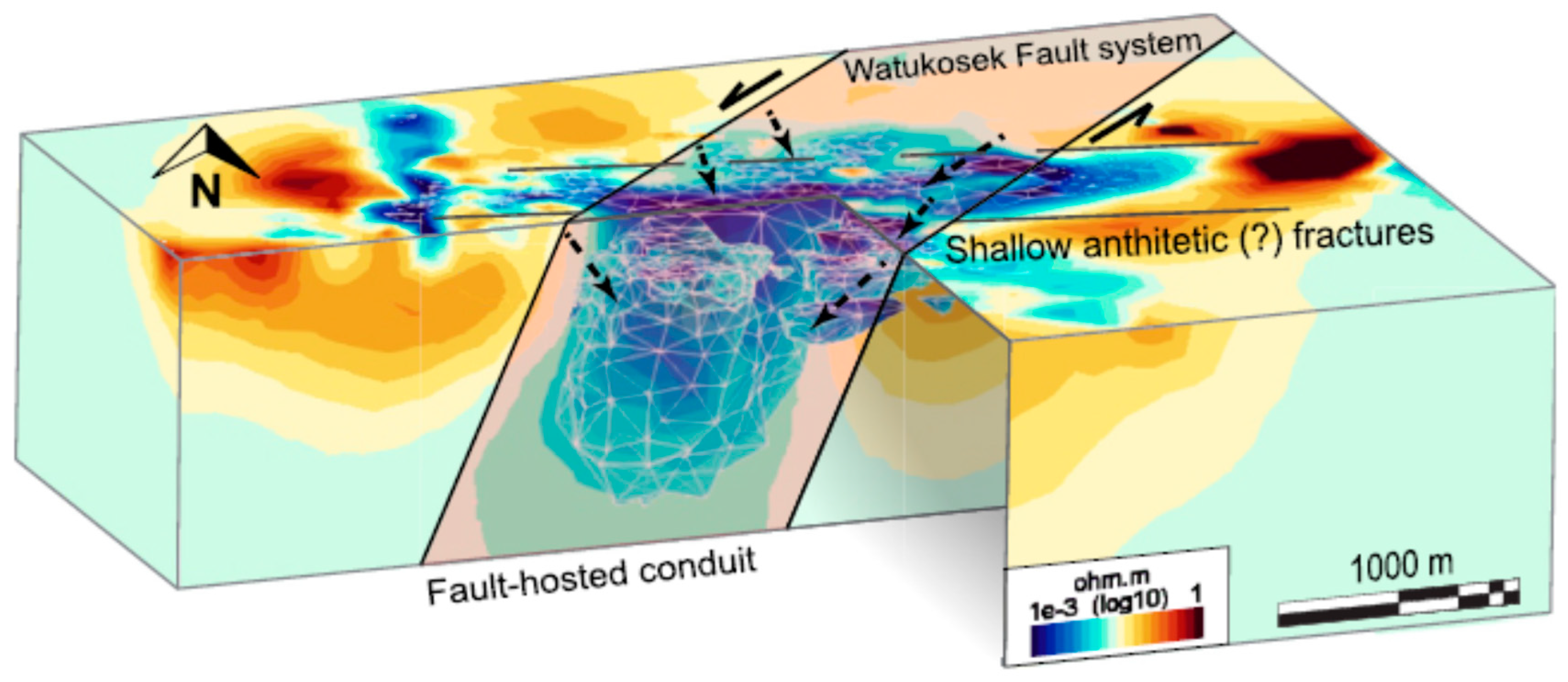
Studies aimed at detecting changes in subsurface resistivity in seismically active areas and their possible relationship to the earthquake cycle find a theoretical basis in the dilatancy–diffusion model [31,32] and reference therein. This is a well-known physical model of precursor phenomena, introduced by the seminal papers of Nur and successively modified and improved by many other authors. It predicts time-dependent changes in the Vp/Vs ratio and subsurface resistivity due to crack opening and fluid diffusion in a volume surrounding the fault system. The faults represent natural pathways for fluid migration, or barriers to movement (Figure 2). The extreme sensitivity of resistivity values to the presence of fluid in the subsurface makes the study of the spatio-temporal patterns of this geophysical parameter in seismically active areas of great interest.
The aim of this review is to critically analyze the current state-of-the-art techniques in the geoelectrical monitoring of subsurface resistivity in seismically active areas under stationary conditions. This study does not consider passive measurements with MT and/or other electromagnetic methods. The MT method has been widely used to map the spatial patterns of subsurface resistivity near active faults [33,34,35,36]. However, there are few examples in the literature of continuous monitoring activities before, during, and after seismic events.
This review will critically analyze both theoretical and experimental aspects of DC resistivity monitoring in seismically active areas, with a focus on the geophysical processes involved in fluid migration near fault structures, the statistical significance of anomalous behavior in resistivity time series, and the various technologies used to design the geoelectrical network.
Finally, an outlook analysis based on recent technological (sensors, IoT, etc.) and methodological (AI-based methods for data processing and tomographic algorithms) developments will be presented and discussed. Novel approaches for real-time monitoring of time-dependent resistivity changes in seismically active zones will be outlined and qualitatively described.
2. DC Geoelectrical Resistivity Method
The DC geoelectrical resistivity method is an old and fascinating geophysical method used across many applicative domains. The resistivity of rocks can be measured by injecting a stationary (DC) current into the ground and detecting the voltage signals generated by the current flow in the subsurface. The DC current is injected into the ground with two electrodes (AB) connected to a power generator, with the current intensity generally ranging from 1 to 10 A. The resulting current produces voltage signals that can be detected on the surface using measuring electrodes (MN). The current energization’s polarity is regularly inverted to minimize the effects of the anthropic electrical noise. The formula ϱa = K × (ΔV/I) can be used to easily obtain the sub-surface’s apparent resistivity. Here, ϱa represents the apparent resistivity, ΔV represents the voltage signal, I is the current intensity, and K is a geometrical factor related to the spatial distribution of the electrodes on the surface [37].
The first applications of this method were based on the use of the vertical electrical sounding (VES) and 1D subsurface models with parallel resistivity layers for data interpretation. Technological advances (e.g., multi-channel arrays, innovative sensors) and novel tomographic algorithms for the 2D and 3D inversion of apparent resistivity values have rapidly transformed the DC geoelectrical method in electrical resistivity tomography (ERT). By moving the energizing and measuring multi-electrode systems along profiles and/or regular grids on the surface, it is possible to obtain 2D and 3D apparent resistivity pseudo-sections. Then, using algorithms for resistivity data inversion, the pseudo-sections can be transformed in 2D and 3D tomographic images [38,39].
To date, the ERT is one of the most robust and popular methods for near-surface geophysical investigations, and has an impressive number of applications, spanning from geohazard assessment to environmental monitoring; from hydrogeology to engineering geology; from hydrogeology to precision farming; and from CO2 storage to the study of the effects of climate change, etc. Furthermore, the introduction of the remote control of sensors and IoT technology allows the capture of sequences of 2D or 3D electrical images, paving the way to studying resistivity changes in the time domain (4D ERT). This new approach has been successfully used to map fluid migration processes in landslides and pollutant transport in groundwater [40,41].
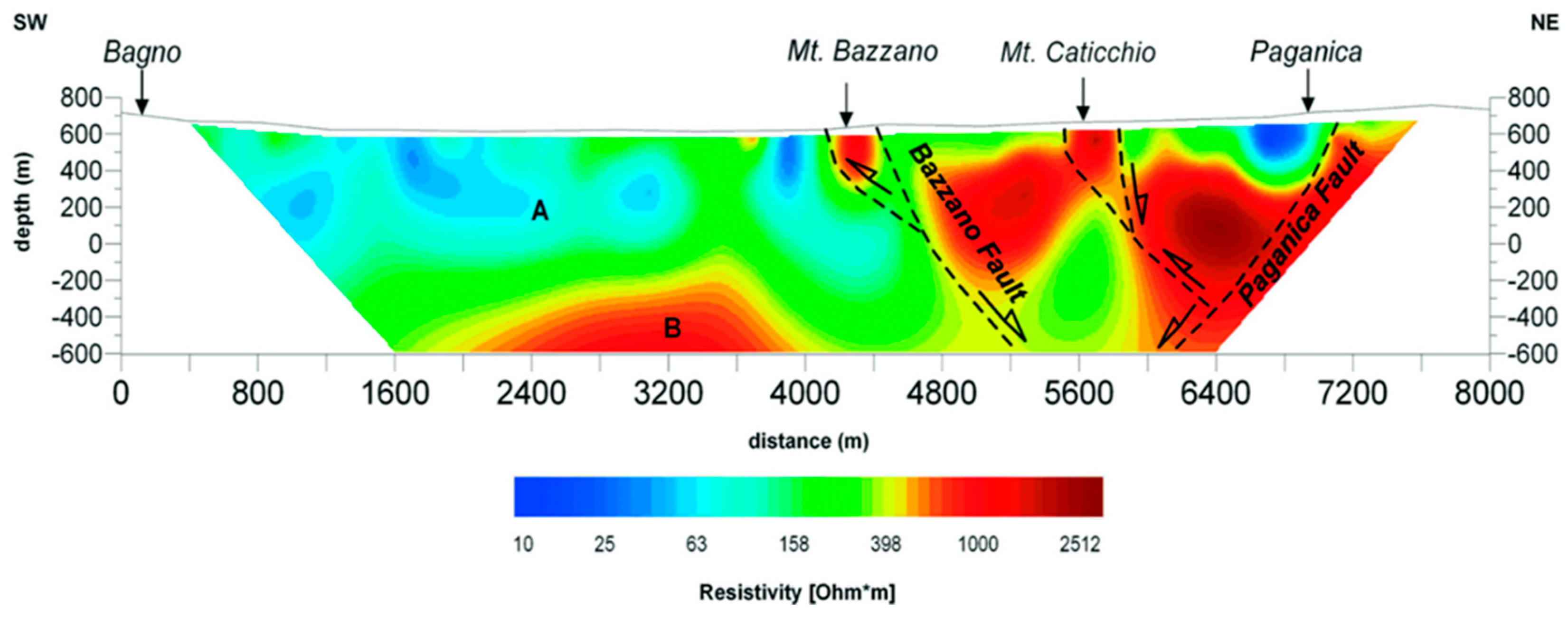
The limit of the ERT method is in its capacity to explore deep geological environments; in large part, its applications are characterized by an exploration depth less than 500 m. This aspect is especially critical in the study of resistivity changes that are possibly related to seismic sequences. The mean depth of the nucleation zone and the surrounding rock is generally greater than that investigated with the ERT method. At present, there are only a few examples in the literature of deep ERTs that have been performed in seismically active areas (Figure 3) and, to our knowledge, there has been no ERT-based continuous monitoring activity of close active faults. Measurements of the resistivity at depths greater than 1 km are possibly only with the magnetotelluric (MT) method, but this is strongly influenced by the presence of anthropic noise. The MT is a passive method based on the study of electrical and magnetic fields measured on the earth’s surface in the frequency range 10−4–104 Hz, and data processing in urbanized areas is strongly affected by electrical noise due to the presence of power lines and/or other man-made noise [33].
3. DC Geoelectrical Observations in Seismic Active Areas
Since the 1960s, in different areas around the world (China, Japan, the USA, and other countries), numerous experiments have been planned and carried out to detect resistivity changes before and during the occurrence of large earthquakes. This paragraph provides an overview of the main results and their schematic classification.
3.1. Long-Term Observations of Apparent Resistivity in China
Since April 1967, the classic Schlumberger array has been used to monitor apparent resistivity at various sites in China [43,44,45,46,47] and references therein. At present, a network of 89 geoelectrical stations is in operation. At each station, four aligned electrodes are used to inject a direct current into the ground and record the voltage signals (Figure 4). Electrodes A and B are used for energization and are located at different distances along the profile, while electrodes M and N are located symmetrically with respect to the center of the profile, and their distance apart is less than 20% of the length of AB. The maximum distance between electrodes A and B is in the range of 1–3 km and, in general, there are two perpendicular arrays at each station.
The apparent resistivity is easily obtained from the formula ϱa = K × (ΔV/I), as described in the previous paragraph. The depth of investigation is related to the maximum distance between electrodes A and B, generally assumed to be about AB/2. The station’s Schlumberger array then measures the apparent resistivity values, and can detect the time dependent changes of the subsurface resistivity within a volume when the radius is less than the investigation depth.
The geoelectrical network of stations located in seismically active areas provides an opportunity to investigate the possible correlations between anomalous patterns in resistivity observations and the occurrence of earthquakes. An impressively large database of apparent resistivity time series is currently available, and many papers analyzing these observations have been published.
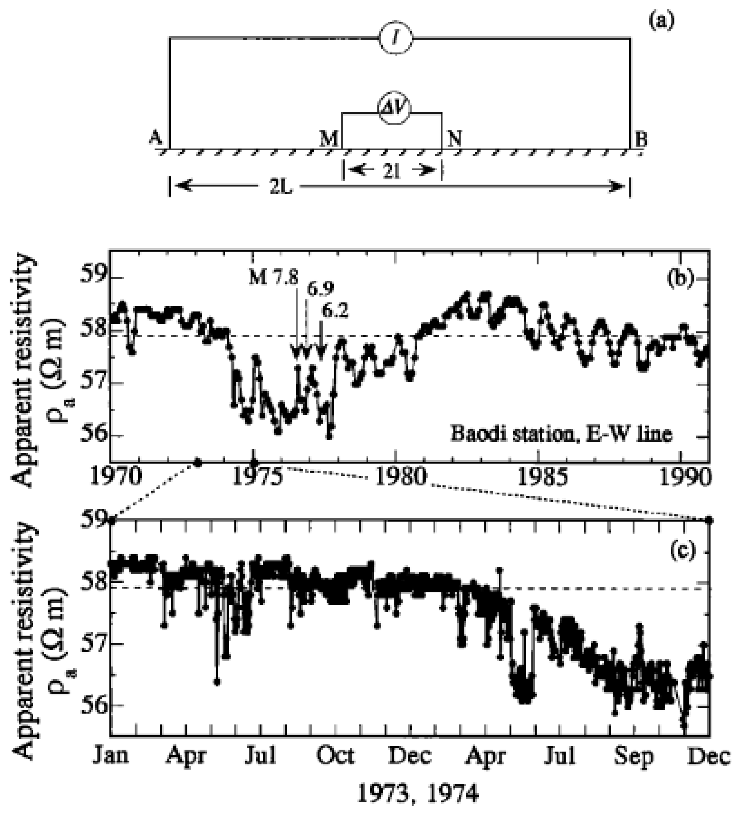
Chu et al. [48] published one of the more interesting seminal papers on this topic, focused on the apparent resistivity changes in a seismically active area located in the northern region of China, which was hit by the 1976 Ms 7.8 Tangshan earthquake. During the period 1974–1976, the analysis identified a spatial pattern of anomalous apparent resistivity changes in many geoelectrical stations located in the source area of the Tangshan earthquake (Figure 5). According to the dilatancy–diffusion model, the shape of the apparent resistivity changes generally represent a constant decrease. After the occurrence of the main shock, the resistivity values increase and reach the baseline level. The comparison of the apparent resistivity values with the hydrological data excludes any correlation and/or influence of rainfall cycles with regards to the geoelectrical data. On the contrary, a co-seismic change in the water table has been clearly detected in deep boreholes.
Recently, some authors have investigated the possible correlation between fault mechanisms, stress fields, and the shape of the spatio-temporal changes in apparent resistivity using the large database available for China. Xie et al. [49] considered the period 1971–2022 and analyzed the anomalous patterns observed in the apparent resistivity time series before 45 Ms 6–6.9 earthquakes with epicenters less than 250 km from the stations. The dataset did not include any aftershocks of magnitude greater than 6 that occurred within 3 months. A set of 61 anomalous patterns in apparent resistivity were observed before 39 out of the 45 examined earthquakes.
A critical analysis of the possible relationship between the shape of the anomalies observed in the apparent resistivity time series and the seismic deformation patterns was carried out. The results were interesting and confirmed that the compressional and dilatancy regimes could be responsible for different time-dependent changes in subsurface resistivity. Of course, no firm conclusions can be drawn about the statistical significance of these anomalous patterns as short-term precursors.
Xie et al. [50] investigated the occurrence of anisotropic changes in apparent resistivity prior to large Ms ≥ 7 earthquakes in China during the period 1967–2021. A group of 16 Ms ≥ 7 earthquakes with epicenters within 400 km of the geoelectric monitoring stations was selected, and their focal mechanisms were evaluated. From the analysis of the apparent resistivity values observed by the geoelectrical network, a database of 39 anomalous patterns prior to the occurrence of 13 earthquakes was identified, with a large portion of these changes showing the same anisotropic pattern. For a single station, the array with a larger angle in relation to the P-axis had a larger magnitude of change, while the array with a smaller angle in relation to the P-axis had a smaller magnitude of change, or even an imperceptible change. The study confirmed the influence of compressional regimes on anomalous resistivity patterns, as tested in laboratory experiments.
Lu et al. [51] analyzed the apparent resistivity time series observed at three stations located in the area hit by the 12 May 2008 M8.0 Wenchuan earthquake, one of the most destructive seismic events in China in recent decades. They analyzed similarities and differences between the patterns of apparent resistivity changes observed at other stations in the geoelectric network before and during the M7.8 Tangshan and M7.2 Songpan earthquakes (Figure 6).
During the 2 years before the mainshock, a slow decrease was observed at the Pixian station, located close to the epicentral zone (about 35 km). During the coseismic phase, only a small time-dependent change in the apparent resistivity values was observed. On the contrary, a clear coseismic anomalous pattern was observed at Jiangyou station (about 150 km from the epicenter). Finally, no time-dependent changes in apparent resistivity values were observed at Wudu station (300 km from the epicenter). A detailed analysis of the faulting mechanisms and the earth stress field near the stations was carried out, and their possible relationship with the apparent resistivity patterns was discussed.
Based on these recent studies, firm conclusions about the statistical significance of these anomalous patterns as short-term precursors cannot be established. However, these recent papers have examined the complex relationship between the pattern of the mechanical stress field and the shape of anomalous apparent resistivity signals, which could possibly be related to impending earthquakes.
3.2. Monitoring of Resistivity with Large Telluric Arrays in California
The first pioneering experiments were carried out in California in the early 1970s in order to detect potential variations in apparent resistivity values near the San Andreas fault. The first experiment was conducted using a DC geoelectric station installed near the small town of Hollister [27]. In this area, an M = 4 earthquake occurred in June 1973, and during the monitoring activity, a change in the apparent resistivity values was detected.
Following these initial encouraging results, geoelectrical monitoring was upgraded and implemented in successive years [52]. A large network of transmitting and receiving electrode systems was installed. The emitting stations were able to inject a DC square-wave current with an intensity up to a maximum of 100 A into the ground, and the maximum distance between the stations was 20 km. Accurate signal processing was performed to evaluate the errors associated with the estimate of the apparent resistivity values and to detect the influence of external noise, such as groundwater level and telluric noise. However, no significant anomalous patterns in the apparent resistivity values were observed during the period of 1975–1979, and no changes were detected in response to an M = 4 earthquake that occurred near the San Andreas fault south of Hollister, the same zone affected by the 1973 earthquake. The main results were the implementation of an advanced technological system for monitoring DC apparent resistivity values, and the development of a methodological approach for removing external electrical noise and reducing errors associated with the estimate of the apparent resistivity.
After these preliminary field experiments, Park and Fitterman [53] clearly described and analyzed the results of long-term geoelectrical monitoring activity in Parkfield, an area affected by the San Andreas fault. Previous seismological studies had indicated that a moderate earthquake had occurred in this zone every 22 ± 5 years. Additionally, this area was characterized by the presence of a dense sensor network for geophysical, geochemical, and geodetic measurements, with the aim to evaluate pre- and post-seismic phenomena. Therefore, the study area was an ideal outdoor laboratory to test the possible application of apparent resistivity as a short-term earthquake precursor.
At Parkfield, a geoelectrical network was established consisting of six transmitting systems with an electrode separation of approximately 1000 m and eight receiving systems with an electrode distance ranging from 4 to 16 km (Figure 6). The energizing dipoles were utilized to characterize the subsurface resistivity structures, while the receiving dipoles facilitated the mapping of the temporal fluctuations of the telluric signals. The basic principle of the telluric method is that the electrical fields simultaneously measured at two different sites are related by a transfer function, under the assumption that the induced magnetic fields are coherent between the stations. The transfer function is related to the subsurface resistivity pattern of the investigated area. Thus, changes in subsurface resistivity structure can be detected by analyzing the telluric variations.
In fact, the purpose of this network was to detect changes in telluric signals (voltage measurements on the subsurface in the absence of energization) resulting from modifications in the subsurface resistivity pattern before and during an earthquake.
A sensitive analysis was conducted to determine the minimum detectable change in apparent resistivity based on the analysis of telluric signals recorded by the network. The subsurface resistivity pattern was obtained using the vertical electrical sounding (VES) method to investigate shallow layers, while the large dipoles of the geoelectrical network were used to investigate deep geological structures. The apparent resistivity values were interpreted objectively using a forward approach based on the 3D finite difference method [54]. The subsurface of the study area exhibited low resistivity values and a high degree of variability, which can be attributed to the presence of weathered and fractured materials. Based on the sensitivity analysis results, it was proposed that the geoelectrical network was potentially able to detect telluric changes caused by variations in resistivity in a zone located at depths between 1 and 6 km, where the earthquake epicenters were located.
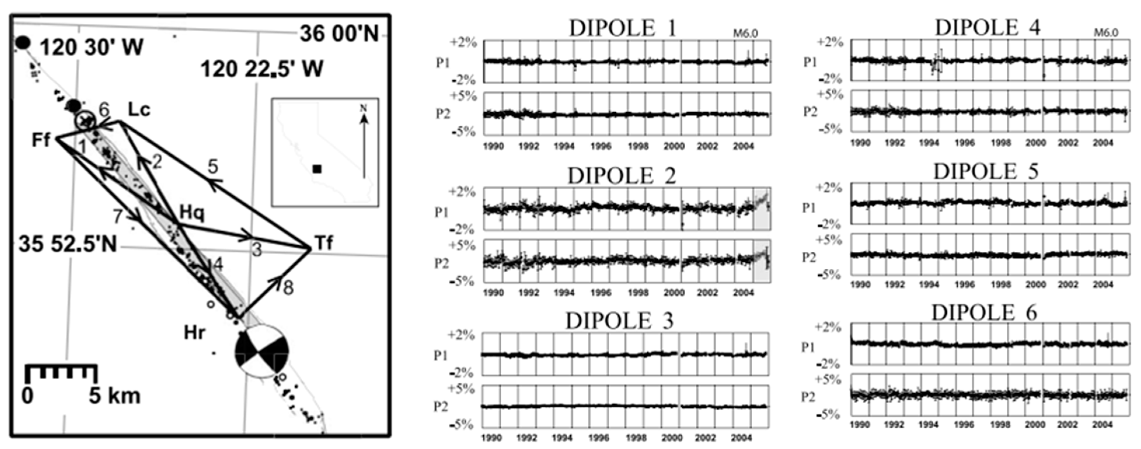
The geoelectrical network installed at Parkfield facilitated the detection of telluric time-dependent fluctuations over a long period. The voltages measured at dipoles one through six were considered to be a linear combination of the voltages measured at dipoles seven and eight, which were used as references for the other dipoles. The dimensionless coefficients of this relation were identified as telluric coefficients. A robust statistical analysis of the projections P1 and P2 of the telluric coefficients onto the average autovectors of the matrix of the telluric coefficients was carried out across the monitoring period from 1990 to 2005 (Figure 7). Projections P1 and P2 were related to the variations perpendicular and parallel to the fault, respectively.
A M = 6 earthquake occurred at Parkfield after a period of systematic observations with the large telluric array. The hypocenter was 8 km beneath the telluric array. Park et al. [23] critically analyzed the results of more than 20 years of systematic monitoring. No significant changes in the telluric projections P1 and P2 were observed prior to or during the seismic event. Additionally, the researchers utilized the earthquake’s slip estimate and Okada’s dislocation model to assess the volumetric strain and the associated resistivity changes. The simulation confirmed that the telluric sensors can detect resistivity changes caused by mechanical stress. The results of the Parkfield experiment and the absence of other significant DC resistivity monitoring activities in the USA has discouraged the scientific community, and inhibited the possibility of using subsurface resistivity for short-term earthquake prediction.
3.3. DC Resistivity Measurements in Japan
One of the earliest studies on time-dependent changes in rock resistivity measured in seismic areas was conducted in Japan. At the Aburatsubo observatory, located in a coastal area of the Miura Peninsula (Japan), a geoelectrical station was installed to detect the rate of resistivity variations. The physical principle adopted in the study was similar to that used in other studies, but the monitoring dimensions were completely different. The electrodes were spaced 2 m apart, and the current intensity was approximately 100 mA. As a result, the apparatus was able to measure resistivity changes in shallow layers. The first observations were made in the late 1960s by Yamazaki [55,56,57].
The analysis of the continuous apparent resistivity values recorded by the station revealed a set of 11 stepwise changes corresponding to strong seismic events. The resistivity variations were found to be linearly correlated with the strain rate in the direction of the electrodes. A sensitivity check was performed, considering the tidal effects. The results confirmed the high sensitivity of the geoelectrical station, and its ability to detect mechanical strain. However, the available data did not allow for definitive conclusions regarding the occurrence of pre-seismic signals or the mechanism behind the observed step changes in resistivity values (Figure 8).
After several years, a retrospective analysis of the initial measurements, along with the acquisition of new data at the same site following a technological upgrade of the station, were carried out. A cross-check analysis with other geophysical parameters such as temperature and rainfall clearly demonstrated that the polarity of the coseismic resistivity changes was influenced by seasonal effects. Furthermore, the step variations in the resistivity time series appeared to be correlated to the arrival of S waves, and the pre-seismic changes in the resistivity values were found to be present only by chance, and without any statistical significance [58].
3.4. DC Resistivity Measurement in Russia
The first observations of time-dependent changes in subsurface resistivity parameters in Russia date back to 1967, when a geoelectrical monitoring station was installed in the Pamir region [59]. A dipole–dipole array was used, with a distance of 6 km between the emitting (AB) and receiving (MN) electrode systems, a dipole length of 300–500 m, and a square-wave current of 100 A regularly injected into the ground. During the first few years of monitoring, slow decreases in apparent resistivity values were observed, corresponding to local earthquakes. These effects were associated with an increase in fluid pore pressure. However, in the absence of comparison with other geophysical data and robust statistical analysis, no significant results were obtained.
Barsukov et al. [60] re-analyzed the data from 1967–1972 and introduced new models to interpret the possible correlation between resistivity changes and local earthquakes. They analyzed the investigation depth of the dipole electrical sounding and its capacity to map resistivity patterns within a depth range of 0–3 km. The investigation depth was generally half of the dipole distance. The study confirmed that the anomalous patterns in resistivity time series had a local origin, likely caused by fluid migration within fractured zones with high permeability along fault structures. However, there are still ambiguities regarding the statistical significance of pre-seismic variations in electrical resistivity (Figure 9).
Another study was conducted in the Gorny Altau Basin, which was affected by the 2003 Mw7.3 Chuya earthquake. Geoelectrical soundings (VES and dipole–dipole arrays) and the transient electromagnetic method (TEM) were used to reconstruct the subsurface resistivity pattern of the study area [61]. Accurate measurements were obtained during the post-seismic period. The results confirmed the need to map changes in the subsurface resistivity distribution on a large scale. The observations were limited to detecting only local resistivity changes in shallow layers.
3.5. Monitoring of Apparent Resistivity in Areas with Mechanical Loading Changes Due to Anthropic Activities
It is widely recognized that the construction of dams can induce local seismic activity. The best-known example is the Koyna dam in India [62]. The mechanical loading of the water impoundment and its changes over time create a stress field in the surrounding areas that can cause microcracks and fractures. This in turn can change the pore pressure and activate pre-existing faults in seismic zones. In addition, the presence of large dams has been observed to cause variations in other geophysical parameters.
One of the most important parameters is the apparent resistivity. A pioneering study was carried out in a seismic zone of the Northern Caucasus, where many hydroelectrical stations were installed. The Chirkey dam created a water reservoir with a volume of 2.9 km3, with seasonal variations of the water level ranging up to 35–40 m. In 1975, after the filling of the dam, a dipole–dipole electrical sounding method was used to regularly monitor the apparent resistivity of the subsurface [63]. Measurements were performed at various stations located at distances ranging from 1.6 km to 11.3 km from the dam. A DC current with an intensity of 240 A and a regular change of polarity was injected into the ground, and the length of the energizing dipole was 750 m. Between 1977 and 1989, a clear decrease in apparent resistivity was observed at two monitoring stations. The resistivity variations were more consistent during the period of 1977–1978 as compared to those observed during 1988–1989. A correlation appeared to exist on a weekly basis between the release of seismic energy near the dam location and the changes in apparent subsurface resistivity. However, due to the complexity of the phenomena, no firm conclusions could be drawn (Figure 10).
In the same area, Idarmachev et al. [64] studied the time-dependent changes in apparent resistivity in a well located on the right side of the Chirkey dam (Figure 11). They observed a significant increase in local seismicity after the reservoir was filled with water. The apparent resistivity in the well was measured using a probe with a classical four-electrode array. Electrodes A and B were installed at depths of 90 m and 99 m, respectively, with a distance of 9 m between them. The upper electrode was positioned 30 m below the minimum seasonal water level in the well, and it was found that the resistance of the water in the well had a negligible influence. Multi-year monitoring of the apparent resistivity was conducted. The correlation between the resistivity and water level with a 12-day shift was noteworthy. Sharp decreases in resistivity were generally associated with rises in the water level, while slight increases were observed during unloading phases. The shift suggested that changes in rock resistivity are not directly related to water level, but they are influenced by hydromechanical or seepage processes related to cyclic water level fluctuations.
Another field experiment was conducted at the Sur-Fretes ridge on the French Alps. The ridge, situated between two artificial lakes, provides a natural laboratory for studying geophysical phenomena associated with the deformation of a rock system under mechanical loading and hydrological stress. The initial findings focused on the spatial and temporal variability of self-potential (SP) signals [65]. The SP method is based on the observation of the natural electrical field on the Earth’s surface; the movements of fluids rich in electrical cations can produce electrical signals. In tectonic areas, the flow of groundwater generates an electric current of electrokinetic nature, known as the streaming current. This current is associated with the drag of the excess of charge located near the surface of the minerals. In the liquid pore water, the streaming current generates an electrical field (the streaming potential) that can be remotely recorded at the ground surface of the Earth (or in boreholes).
In a subsequent phase, Hautot [66] analyzed the correlation between changes in electrical resistivity and variations in pore pressure over time. The study utilized an array of 20 dipoles to detect the natural electrical field and an MT station. The induced electrical field distortion was caused by resistivity heterogeneity in the local subsurface. By analyzing the temporal variations in the distortion effects, it was possible to reconstruct changes in subsurface resistivity. The results indicated that 20% of the observed resistivity variations were associated with pore pressure and cracks modulated by the stress field.
Finally, other experiments were carried out at the Balapan site of the Semipalatinsk test site used for underground nuclear explosions in Kazakhstan [67]. Periodic electric surveys allowed the exploration and localization of two zones with changeable rock electroconductivity, discriminating between the fluid movements coming from the deep geological environment and the shallow waters related to atmospheric precipitation.
4. Discussion
A summary of the main technological and methodological aspects of the geoelectrical monitoring activities carried out in different worldwide seismotectonic areas is reported in Table 1.
The field experiments carried out in China since the 1960s, which have continued for many decades, represent the most relevant activity; to date, geoelectrical monitoring activity continues to be in operation, and about 80 stations are collecting apparent resistivity values with a Schlumberger array. However, their observations are characterized by a limited depth of investigation (less than 1 km), and their spatial distribution is extremely poor considering the geographical extent of the study area. The results have a local character, and there is a systematic lack of robust statistical analysis. In any case, some anomalous patterns observed before large earthquakes seem to confirm the dilatancy–diffusion model as the most reliable geophysical process underlying the variation of the apparent resistivity before, during, and after the occurrence of seismic events.
Another long-period monitoring activity was carried out in California, at the Parkfield test site, which can be considered one of the most interesting natural laboratories for verifying pre-seismic electrical resistivity variations. Despite some preliminary successes, the large telluric array installed in this area did not observe any resistivity signals prior to the M = 6 earthquake, which had an epicenter below the center of the array. Great attention was paid to the development of robust statistical analysis for detecting time-dependent changes in the telluric coefficients related to possible subsurface resistivity variations in the investigated area; however, during the entire monitoring period (1990–2005), no pre-seismic resistivity changes were observed. It is noteworthy that the telluric array was completely passive, and the resistivity variations in the subsurface could be detected only by the distortion of the electrical potential recorded by the large dipoles. Consequently, the array captured only “integral features” of the apparent resistivity structure.
Many other experiments have been carried out in Japan, Russia, and other seismically active areas of the world, but all the measurements have been only of local relevance, and the observation periods were not regular. On the contrary, the DC resistivity monitoring activities carried out in the areas affected by induced seismicity due to the presence of large dams clearly demonstrated the triggering role of mechanical loading in producing resistivity variations. In geological environments characterized by active faults where fractured zones with the presence of fluid existed, the resistivity variations were clearly related to changes in the water storage level. These activities confirmed the basic principles of the dilatancy–diffusion model, and the results of the related laboratory experiments.
With regards to the technological features, it is necessary to underline the absence of standard rules and protocols for geoelectrical data acquisition in seismically active areas. The DC resistivity method is largely applied in near-surface exploration, and the technologies for this activity are robust and well assessed. Unfortunately, geoelectrical investigations in seismic areas have been carried out using many different approaches and strategies (Table 1).
This review aims to encourage the initiation of new DC resistivity monitoring activities in seismically active areas. In the last two decades, the subsurface resistivity pattern in seismically active areas has been studied using mainly the ERT and MT methods, contributing to a better understanding of the geometry of fault systems. The ERT method produces high-resolution images of the surface evidence of active faults, while the MT method depicts resistivity images of deep fault systems. However, the MT method has limitations due to its low spatial resolution and the influence of man-made noise. Furthermore, there are no seismic zones where the ERT and MT methods are currently applied for studying resistivity changes in the spatial and temporal domains. The technological development of geoelectrical data acquisition systems and the availability of IoT-based procedures for remote sensor control are critical for the implementation of new DC resistivity monitoring networks designed to operate in real-time and collect sequences of tomographic images [68]. This represents an extraordinary opportunity to better investigate the fluid migration processes that play a key role in earthquake generation mechanisms.
Furthermore, this review highlighted the lack of robust statistical methods that exist for identifying extreme events and/or anomalous patterns in resistivity time series, which have been tested and validated in various seismological contexts. In a large portion of the experimental studies, there exists no information about the occurrence probability of the anomalous patterns detected in the resistivity observations. The statistical theory underlying the search for extreme events is well assessed and widely applied in many scientific fields. Thus, the lack of a robust evaluation method for the statistical significance of possible precursors is not acceptable. The rapid development of AI and machine learning methods presents an excellent opportunity to enhance the quality of data sharing, processing, and analysis of the resistivity data observed in seismic active areas [69,70].
In this scenario, it is reasonable and possible to develop new strategies for DC resistivity monitoring based on the analysis of historical results, the identification of the main scientific and technological gaps, and the adoption of technological advances and novel methodological approaches. This review suggests that the main pillars of a modern strategy for resistivity measurements in seismic areas could be the following:
- (i)
- The development of DC resistivity monitoring systems for investigating and mapping the subsurface resistivity pattern in a depth range of about 0–5 km. The increase in the investigation depth is fundamental to better characterize the geometry of the fault structures; at present, ERTs are mainly applied for mapping the near-surface evidence of active faults.
- (ii)
- The design of geoelectrical networks capable of obtaining temporal sequences of 3D electrical resistivity tomographic (ERT) images of the subsurface (the time-lapse or 4D ERT is a robust method widely used in hydro-geophysics for shallow investigations). This aspect is crucial to better investigate the fluid migration processes close to the focal zones.
- (iii)
- The planning of a systematic comparison between the resistivity measurements and other geophysical parameters with great attention paid to the Vp/Vs ratio, deformation patterns, and hydro-mechanical parameters. The joint interpretation of resistivity and seismic velocity tomographies could provide new opportunities to better investigate earthquake generation mechanisms.
- (iv)
- The adoption of common procedures for data acquisition and processing, and data sharing in accordance with FAIR and Open Data principles. This is a key issue in regard to promoting the results of best practice examples of monitoring activities. The application of robust statistical methods to assess the probability of the occurrence of anomalous patterns in resistivity observations, and probabilistic evaluation of the possible correlation of these patterns with the occurrence of seismic events, is crucial. The use of AI-based and machine learning methods could provide a great impetus to remove artefacts and/or identify spurious effects relating to these methods.
5. Conclusions
A retrospective analysis of the main results obtained in past decades in the study of DC resistivity monitoring activities in different seismological areas (China, USA, Russia, and Japan) has been carried out. Technological and scientific limits have been analyzed and discussed. Field experiments have confirmed that seismic stress with deformation and crack opening, hydromechanical phenomena, and fluid migration processes can induce resistivity variations in the subsurface. These changes occur in the spatio-temporal domains and can be detected on the surface with a DC geoelectric array. However, it remains difficult to evaluate the possible application of the apparent resistivity as a precursor to earthquakes. The results obtained in different seismic regions of the world are intriguing, but there is much uncertainty about the statistical significance of the observed anomalies. In addition, there is a systematic lack of standard monitoring protocols, and it has been impossible to share and compare the results obtained in different geological and seismic environments.
One of the weak points in the field relates to the absence of a tomographic approach able to describe resistivity patterns at depths relevant to seismic processes. To date, the ERT method has been largely applied to reconstruct the geometry of active faults. There have been no experiments focusing on detecting changes in the temporal domain. Considering the key role of fluid migration in the generation process of earthquakes, the need to follow dynamical variations in the subsurface resistivity appears more relevant.
Another existing scientific gap is the absence of a robust statistical evaluation method for the occurrence probability of anomalous resistivity patterns. This aspect has always produced ambiguities in the analysis of study results, with unfruitful debates in the scientific community reducing the credibility and authority of these studies.
The study of resistivity variations in seismically active areas remains a challenging scientific problem. Thus, it is necessary to completely change the monitoring strategies used, adopting 4D tomographic approaches and AI-based and machine learning methods for statistical data analysis.
Funding
This research received no external funding.
Data Availability Statement
Not applicable.
Acknowledgments
The author thanks Rocchino Caivano for the technical support in the bibliography classification and organization using the WoS database.
Conflicts of Interest
The author declares no conflicts of interest.
References
- Nover, G. Electrical Properties of Crustal and Mantle Rocks—A Review of Laboratory Measurements and their Explanation. Surv. Geophys. 2005, 26, 593–651. [Google Scholar] [CrossRef]
- Palacky, G. Resistivity Characteristics of Geological Targets. In Electromagnetic Methods in Applied Geophysics-Theory; Nabighian, M., Ed.; Society of Exploration Geophysicists: Tulsa, OK, USA, 1987; pp. 53–129. [Google Scholar] [CrossRef]
- Archie, G.E. The electrical resistivity log as an aid in determining some reservoir characteristics. Pet. Trans. AIME 1942, 146, 54–62. [Google Scholar] [CrossRef]
- Johnson, D.L.; Manning, H.J. Theory of Pressure Dependent Resistivity in Crystalline Rocks. J. Geophys. Res. 1986, 91, 11611–11617. [Google Scholar] [CrossRef]
- Johnson, D.L.; Sen, P.N. Dependence of the Conductivity of a Porous Medium on Electrolyte Conductivity. Phys. Rev. B 1988, 33, 3502–3510. [Google Scholar] [CrossRef] [PubMed]
- Colella, A.; Lapenna, V.; Rizzo, E. High-resolution imaging of the High Agri Valley Basin (Southern Italy) with electrical resistivity tomography. Tectonophysics 2004, 386, 29–40. [Google Scholar] [CrossRef]
- Pucci, S.; Civico, R.; Villani, F.; Ricci, T.; Delcher, E.; Finizola, A.; Sapia, V.; De Martini, P.M.; Pantosti, D.; Barde-Cabusson, S.; et al. Deep electrical resistivity tomography along the tectonically active Middle Aterno Valley (2009 L’Aquila earthquake area, central Italy). Geophys. J. Int. 2016, 207, 967–982. [Google Scholar] [CrossRef]
- Lajaunie, J.; Gance, J.; Nevers, P.; Malet, J.P.; Bertrand, C.; Garin, T.; Ferhat, G. Structure of the Sèchilienne unstable slope from large-scale three-dimensional electrical tomography using a Resistivity Distributed Automated System(R-DAS). Geophys. J. Int. 2019, 219, 129–147. [Google Scholar] [CrossRef]
- Perrone, A.; Lapenna, V.; Piscitelli, S. Electrical resistivity tomography technique for landslide investigation: A review. Earth Sci. Rev. 2014, 135, 65–82. [Google Scholar] [CrossRef]
- Mazzini, A.; Carrier, A.; Sciarra, A.; Fischanger, F.; Winarto-Putro, A.; Lupi, M. 3D deep electrical resistivity tomography of the Lusi eruption site in East Java. Geophys. Res. Lett. 2021, 48, e2021GL092632. [Google Scholar] [CrossRef]
- Finizola, A.; Revil, A.; Rizzo, E.; Piscitelli, S.; Ricci, J.; Morin, B.; Angeletti, L.; Mocochain, L.; Sortino, F. Hydrogeological insights at Stromboli volcano (Italy) from geoelectrical, temperature, and CO2 soil degassing investigations. Geophys. Res. Lett. 2006, 33, L17304. [Google Scholar] [CrossRef]
- Bergmann, P.; Schmidt-Hattenberger, C.; Labitzke, T.; Wagner, F.M.; Just, A.; Flechsig, C.; Rippe, D. Fluid injection monitoring using electrical resistivity tomography five years of CO2 injection at Ketzin, Germany. Geophys. Prospect. 2017, 65, 859–875. [Google Scholar] [CrossRef]
- Fitterman, D.V. Theoretical resistivity variations along stressed strike-slip faults. J. Geophys. Res. 1976, 81, 4909–4915. [Google Scholar] [CrossRef]
- Rikitake, T. Earthquake Prediction; Elsevier: New York, NY, USA, 1976; 357p. [Google Scholar]
- Gokhberg, M.B.; Morgounov, V.A.; Pokhtelov, O.A. Earthquake Prediction Seismo-Electromagnetic Phenomena; Gordon and Breach Science Publishers: Amsterdam, The Netherlands, 1995; 193p. [Google Scholar]
- Park, S.K. Monitoring resistivity changes in Parkfield, California: 1988–1995. J. Geophys. Res. 1997, 102, 24545–24559. [Google Scholar] [CrossRef]
- Cicerone, R.D.; Ebel, J.E.; Britton, J. A systematic compilation of earthquake precursors. Tectonophysics 2009, 476, 371–396. [Google Scholar] [CrossRef]
- Brace, W.F.; Orange, A.S. Electrical Resistivity Changes in Saturated Rock under Stress. Science 1966, 153, 1525–1526. [Google Scholar] [CrossRef] [PubMed]
- Brace, W.F.; Orange, A.S. Electrical resistivity changes in saturated rocks during fracture and sliding. J. Geophys. Res. 1968, 73, 1433–1445. [Google Scholar] [CrossRef]
- Takano, M.; Yamada, I.; Fukao, Y. Anomalous electrical resistivity of almost dry marble and granite under axial compression. J. Phys. Earth 1993, 41, 337–346. [Google Scholar] [CrossRef]
- Park, S.K.; Johnston, M.J.S.; Madden, T.R.; Morgan, F.D.; Morrison, H.F. Electromagnetic Precursors in the ULF band: A review of the observations and mechanism. Rev. Geophys. 1993, 31, 117–132. [Google Scholar] [CrossRef]
- Geller, R.J.; Jackson, D.D.; Kagan, Y.Y.; Mulargia, F. Earthquakes Cannot Be Predicted. Science 1997, 275, 1616. [Google Scholar] [CrossRef]
- Park, S.K.; Larsen, J.C.; Lee, T.C. Electrical resistivity changes not observed with the 28 September 2004 M6.0 Parkfield earthquake on the San Andreas fault, California. J. Geophys. Res. 2007, 112, B12305. [Google Scholar] [CrossRef]
- Wyss, M.; Booth, D.C. The IASPEI procedure for the evaluation of earthquake precursors. Geophys. J. Int. 1997, 131, 423–424. [Google Scholar] [CrossRef]
- Qian, F.Y.; Zhao, Y.L.; Yu, M.M.; Wang, Z.X.; Liu, X.W.; Chang, S.M. Geoelectric resistivity anomalies before earthquakes. Sci. Sin. 1983, 26, 326–336. [Google Scholar]
- Zhao, Y.L.; Qian, F.Y.; Yang, T.C.; Liu, J.Y. Experimental in situ of electrical resistivity changes. Acta Seismol. Sin. 1983, 5, 217–225. (In Chinese) [Google Scholar]
- Mazzella, A.; Morrison, H.F. Electrical resistivity variations associated with earthquakes on the San Andreas fault. Science 1974, 185, 855–857. [Google Scholar] [CrossRef] [PubMed]
- Fitterman, D.V.; Madden, T.R. Resistivity observations during creep events at Melendy Ranch, California. J. Geophys. Res. 1977, 82, 5401–5408. [Google Scholar] [CrossRef]
- Park, S.K. Monitoring resistivity changes prior to earthquakes in Parkfield, California with telluric arrays. J. Geophys. Res. 1991, 96, 14211–14237. [Google Scholar] [CrossRef]
- Rikitake, T.; Yamazaki, Y. Resistivity changes as a precursor of earthquake. J. Geomagn. Geoelec. 1976, 28, 497–505. [Google Scholar] [CrossRef]
- Scholz, C.H.; Sykes, L.R.; Aggarwal, Y.P. Earthquake prediction: A physical basis. Science 1973, 181, 803–810. [Google Scholar] [CrossRef] [PubMed]
- Scholz, C.H. The Mechanics of the Earthquakes and Faulting; Cambridge University Press (USA): Cambridge, MA, USA, 1990; 439p, ISBN 0521-33443-8. [Google Scholar]
- Zhdanov, M. Geophysical Electromagnetic Theory and Methods, 1st ed.; Elsevier: Amsterdam, The Netherlands, 2009; ISBN 9780444529633. [Google Scholar]
- Honkura, Y.; Oshiman, N.; Matsushima, M.; Barış, Ş.; Tunçer, M.K.; Tank, S.B.; Çelik, C.; Çiftçi, E.T. Rapid changes in the electrical state of the 1999 Izmit earthquake rupture zone. Nat. Commun. 2013, 4, 2116. [Google Scholar] [CrossRef]
- Karaş, M.; Tank, S.B.; Özaydın, S. Electrical conductivity of a locked fault: Investigation of the Ganos segment of the North Anatolian Fault using three-dimensional magnetotellurics. Earth Planets Space 2017, 69, 107. [Google Scholar] [CrossRef]
- Balasco, M.; Cavalcante, F.; Romano, G.; Serlenga, V.; Siniscalchi, A.; Stabile, T.A.; Lapenna, V. New insights into the High Agri Valley deep structure revealed by magnetotelluric imaging and seismic tomography (Southern Apennine, Italy). Tectonophysics 2021, 808, 228817. [Google Scholar] [CrossRef]
- Koefoed, O. Geosounding Principles 1: Resistivity Sounding Measurements; Elsevier: Amsterdam, The Netherlands, 1979. [Google Scholar]
- Loke, M.H.; Chambers, J.E.; Rucker, D.F.; Kuras, O.; Wilkinson, P.B. Recent developments in the direct-current geoelectrical imaging method. J. Appl. Geophys. 2013, 95, 135–156. [Google Scholar] [CrossRef]
- Loke, M.H.; Barker, R.D. Rapid least-squares inversion of apparent resistivity pseudosections using a quasi-Newton method. Geophys. Prospect. 1996, 44, 131–152. [Google Scholar] [CrossRef]
- Lapenna, V.; Perrone, A. Time-Lapse Electrical Resistivity Tomography (TL-ERT) for Landslide Monitoring: Recent Advances and Future Directions. Appl. Sci. 2022, 12, 1425. [Google Scholar] [CrossRef]
- Binley, A.; Henry-Poulter, S.; Shaw, B. Examination of solute transport in an undisturbed soil column using electrical resistance tomography. Water Resour. Res. 1996, 32, 763–769. [Google Scholar] [CrossRef]
- Balasco, M.; Galli, P.; Giocoli, A.; Gueguen, E.; Lapenna, V.; Perrone, A.; Piscitelli, S.; Rizzo, E.; Romano, G.; Siniscalchi, A.; et al. Deep geophysical electromagnetic section across the middle Aterno Valley (central Italy): Preliminary results after the 6 April 2009 L’Aquila earthquake. Boll. Geofis. Teor. Appl. 2011, 52, 443–455. [Google Scholar] [CrossRef]
- Qian, F.; Zhao, Y.; Xu, T. An analysis of the seasonal variation of disturbance in georesistivity. Acta Seismol. Sin. 1988, 1, 69–83. [Google Scholar] [CrossRef]
- Qian, F.; Zhao, Y.; Xu, T.; Ming, Y.; Zhang, H. A model of an impending- earthquake precursor of geoelectricity triggered by tidal forces. Phys. Earth Planet. Inter. 1990, 62, 284–297. [Google Scholar] [CrossRef]
- Qian, G. The Great China Earthquake; Foreign Languages Press: Beijing, China, 1989; 354p. [Google Scholar]
- Qian, J. Regional study of the anomalous change in apparent resistivity before the Tangshan earthquake (M 7.8, 1976) in China. Pure Appl. Geophys. 1985, 22, 901–920. [Google Scholar] [CrossRef]
- Lu, J.; Qian, F.Y.; Zhao, Y.L. Sensitivity analysis of the Schlumberger monitoring array: Application to changes of resistivity prior to the 1976 earthquake in Tangshan, China. Tectonophysics 1999, 307, 397–405. [Google Scholar] [CrossRef]
- Chu, J.J.; Gui, X.T.; Dai, J.A.; Marone, C.; Spiegelman, M.W.; Seeber, L.; Armbruster, J.G. Geoelectric signals in China and the earthquake generation process. J. Geophys. Res.-Solid Earth 1996, 101, 13869–13882. [Google Scholar] [CrossRef]
- Xie, T.; Ying, H.; Qing, Y.; Yan, X. Changes and mechanisms of apparent resistivity before earthquakes of MS6.0–6.9 on the Chinese mainland. Front. Earth Sci. 2023, 11, 1187660. [Google Scholar] [CrossRef]
- Xie, T.; Xue, Y.; Ye, Q.; Lu, J. Anisotropic change in apparent resistivity before earthquakes of M (S) > 7.0 in China mainland. Geomat. Nat. Hazards Risk 2022, 13, 1207–1228. [Google Scholar] [CrossRef]
- Lu, J.; Xie, T.; Li, M.; Wang, Y.L.; Ren, Y.X.; Gao, S.D.; Wang, L.W.; Zhao, J.L. Monitoring shallow resistivity changes prior to the 12 May 2008 M 8.0 Wenchuan earthquake on the Longmen Shan tectonic zone, China. Tectonophysics 2016, 675, 244–257. [Google Scholar] [CrossRef]
- Morrison, H.F.; Fernadez, R. Temporal Variations in the Electrical Resistivity of the Earth’s crust. J. Geophys. Res. 1986, 91, 11–618. [Google Scholar] [CrossRef]
- Park, S.K.; Fitterman, D.V. Sensitivity of the telluric monitoring array in Parkfield, California, to changes of resistivity. J. Geophys. Res. 1990, 95, 15557–15571. [Google Scholar] [CrossRef]
- Dey, A.; Morrison, H.F. Resistivity modeling for arbitrarily shaped three-dimensional structures. Geophysics 1979, 44, 753–780. [Google Scholar] [CrossRef]
- Yamazaki, Y. Electrical conductivity of strained rocks, the fourth paper, Improvement of the resistivity variometer. Earthquake Res. Inst. Bull. Univ. Tokyo 1968, 46, 957–964. [Google Scholar]
- Yamazaki, Y. Coseismic resistivity steps. Tectonophysics 1974, 22, 159–171. [Google Scholar] [CrossRef]
- Rikitake, T.; Yamazaki, Y. Precursory and coseismic changes in ground resistivity. J. Phys. Earth 1977, 25, S161–S173. [Google Scholar] [CrossRef]
- Utada, H.; Yoshino, T.; Okubo, T.; Yukutake, T. Seismic resistivity changes observed at Aburatsubo, central Japan, revisited. Tectonophysics 1998, 299, 317–331. [Google Scholar] [CrossRef]
- Barsukov, O.M. Variations of electric resistivity of mountain rocks connected with tectonic causes. Tectonophysics 1972, 14, 273–277. [Google Scholar] [CrossRef]
- Barsukov, P.; Fainberg, E. New interpretation of the reduction phenomenon in the electrical resistivity of rock masses before local earthquakes. Phys. Earth Planet. Inter. 2019, 294, 106279. [Google Scholar] [CrossRef]
- Nevedrova, N.N.; Sanchaa, A.M.; Shalaginov, A.E.; Babushkin, S.M. Electromagnetic monitoring in the region of seismic activization (on the Gorny Altai (Russia) example). Geod. Geodyn. 2019, 10, 460–470. [Google Scholar] [CrossRef]
- Talwani, P. Seismotectonics of the Koyna-Warna Area, India. Pure Appl. Geophys. 1997, 150, 511–550. [Google Scholar] [CrossRef]
- Idarmachev, S.G.; Arefiev, S.S. Results of dipole electric sounding in the area of the Chirkey water reservoir after its filling. Izv. Phys. Solid Earth 2009, 45, 802–811. [Google Scholar] [CrossRef]
- Idarmachev, I.S.; Deshcherevskii, A.V.; Idarmachev, S.G. Assessment of the Relationship Between Water Level Changes in the Chirkei Reservoir and Electrical Resistivity of Rocks in the Right Bank Region of the Hydropower Plant Dam. Power Technol. Eng. 2019, 53, 278–283. [Google Scholar] [CrossRef]
- Trique, M.; Richon, P.; Perrier, F.; Avouac, J.; Sabroux, C. Radon emanation and electric potential variations associated with transient deformation near reservoir lakes. Nature 1999, 399, 137–141. [Google Scholar] [CrossRef]
- Hautot, S. Modeling temporal variations of electrical resistivity associated with pore pressure change in a kilometer-scale natural system. Geochem. Geophys. Geosystems 2005, 6, 615. [Google Scholar] [CrossRef]
- Stromov, V.M.; Kabailov, A.N.; Drozdov, A.V. Results of regime electric survey at Balapan Site. NNC RK Bull. 2005, 2, 95–100. (In Russian) [Google Scholar]
- Balasco, M.; Lapenna, V.; Rizzo, E.; Telesca, L. Deep Electrical Resistivity Tomography for Geophysical Investigations: The State of the Art and Future Directions. Geosciences 2022, 12, 438. [Google Scholar] [CrossRef]
- Yu, S.; Ma, J. Deep learning for geophysics: Current and future trends. Rev. Geophys. 2021, 59, e2021RG000742. [Google Scholar] [CrossRef]
- Bergen, K.J.; Johnson, P.A.; de Hoop, M.V.; Beroza, G.C. Machine learning for data-driven discovery in solid Earth geoscience. Science 2019, 22, eaau0323. [Google Scholar] [CrossRef] [PubMed]
Figure 1.
Variability range of the electrical resistivity of various rock types (after [2]).
Figure 1.
Variability range of the electrical resistivity of various rock types (after [2]).

Figure 2.
Electrical imaging of a Watukosek fault system in a volcanic area located in the East Java Basin (Indonesia), representing the largest eruptive clastic system on Earth. The possibility of the presence of shallow anthitetic fractures has been hypothesised [9].
Figure 2.
Electrical imaging of a Watukosek fault system in a volcanic area located in the East Java Basin (Indonesia), representing the largest eruptive clastic system on Earth. The possibility of the presence of shallow anthitetic fractures has been hypothesised [9].

Figure 3.
Deep electrical resistivity tomography carried out in the epicentral area of the 2009 Abruzzo earthquake (central Italy). (A) represents alluvial deposits and the Messinian turbidite complex; (B) represents unfractured calcareous block. The more resistive blocks are probably associated to Miocene units. Black dashed lines indicate presumed faults [42].

Figure 4.
Schematic diagram of a geoelectrical network installed in China. The station is equipped with two perpendicular Schlumberger arrays, A and B represent the electrodes for current injection, while M and N are the electrodes for the voltage measurements [47,48].

Figure 5.
Temporal variations of the apparent resistivity, measured with a Schlumberger array at Baodi station, which is located close to the epicentral area of the 7.8 1976 Tangshan earthquake. At the top, the long-term variations of the apparent resistivity are displayed. On the top of the figure (a), it is depicted the geometry of the electrode array. In the central part (b), the apparent resistivity values measured with the array oriented in E-W direction are displayed. At the bottom (c), a zoomed in chart of the observations recorded during 1974 is shown [46,47].

Figure 6.
Temporal variations of the apparent resistivity observed at three monitoring stations (Wudu, Jiangyou, Pixian) of the Chinese network at different distances (300 km, 150 km, 35 km) form the epicentral area of the M8.0 Wenchuan earthquake [51]. The grey zone highlights the sharp variation of the apparent resistivity data, the red lines indicate the sequence of the seismic events.

Figure 7.
Schematic diagram of the dipole array installed at Parkfield (California), and telluric signals recorded during the period 1990–2005 at different receiving stations of the geoelectrical network [23]. The numbers identify the different dipoles of the geoelectrical monitoring network.
Figure 7.
Schematic diagram of the dipole array installed at Parkfield (California), and telluric signals recorded during the period 1990–2005 at different receiving stations of the geoelectrical network [23]. The numbers identify the different dipoles of the geoelectrical monitoring network.

Figure 8.
On the left, the diagram of the technological system used to measure resistivity and accelerometric signals at the Aburatsubo observatory is displayed. On the right, the coseismic changes in resistivity, in correspondence to an M6.6 earthquake, are reported [58].
Figure 8.
On the left, the diagram of the technological system used to measure resistivity and accelerometric signals at the Aburatsubo observatory is displayed. On the right, the coseismic changes in resistivity, in correspondence to an M6.6 earthquake, are reported [58].

Figure 9.
Temporal variations of the apparent resistivity observed by means of a large dipole–dipole array located close a complex fault system in the Pamir region, and release of seismic energy [60].
Figure 9.
Temporal variations of the apparent resistivity observed by means of a large dipole–dipole array located close a complex fault system in the Pamir region, and release of seismic energy [60].

Figure 10.
Correlation between energy seismic release and apparent resistivity values observed at geoelectrical stations located close to the Chirkey dam [63]. The numbers identify the main seismic event.
Figure 10.
Correlation between energy seismic release and apparent resistivity values observed at geoelectrical stations located close to the Chirkey dam [63]. The numbers identify the main seismic event.

Figure 11.
Seasonal fluctuations of the apparent resistivity values (labelled with 1 in the figure) related to changes in the water storage level (labelled with 2) of the Chirkey dam (Northen Caucasus) [64].
Figure 11.
Seasonal fluctuations of the apparent resistivity values (labelled with 1 in the figure) related to changes in the water storage level (labelled with 2) of the Chirkey dam (Northen Caucasus) [64].


Table 1.
Main characteristics of the geoelectrical monitoring activities.
| Study Area | Monitoring Network | Observed Parameters | Main Results |
|---|---|---|---|
| Seismotectonic zones in China | Schlumberger array | Apparent resistivity in the shallow layers | Study of the correlation between focal mechanisms and shape of the resistivity patterns |
| San Andreas fault (Parkfield, California) | Large dipole–dipole arrays for passive measurements | Telluric signals related to the resistivity changes in subsurface | Robust statistical analysis of the telluric signals during pre and post seismic phases |
| Miura Peninsula (Japan) | Resistivity variometers | Apparent resistivity variations in very shallow layers | Sensitivity tests and study of the influence of the tidal effects |
| Pamir and Altai–Sayan regions (Russia) | Large dipole–dipole arrays for active measurements | Apparent resistivity of deep geological layers | Resistivity changes due to the fluid migration in high permeability zones |
| Surrounding areas near large dams located in France and North Caucasus (Russia) | Geoelectrical arrays installed on surface and in boreholes | Apparent resistivity at different depths | Analysis of the influence of mechanical loading and pore pressure on the resistivity values |
Disclaimer/Publisher’s Note: The statements, opinions and data contained in all publications are solely those of the individual author(s) and contributor(s) and not of MDPI and/or the editor(s). MDPI and/or the editor(s) disclaim responsibility for any injury to people or property resulting from any ideas, methods, instructions or products referred to in the content. |
© 2024 by the author. Licensee MDPI, Basel, Switzerland. This article is an open access article distributed under the terms and conditions of the Creative Commons Attribution (CC BY) license (https://creativecommons.org/licenses/by/4.0/).
Share and Cite
MDPI and ACS Style
Lapenna, V. Detecting DC Electrical Resistivity Changes in Seismic Active Areas: State-of-the-Art and Future Directions. Geosciences 2024, 14, 118. https://0-doi-org.brum.beds.ac.uk/10.3390/geosciences14050118
AMA Style
Lapenna V. Detecting DC Electrical Resistivity Changes in Seismic Active Areas: State-of-the-Art and Future Directions. Geosciences. 2024; 14(5):118. https://0-doi-org.brum.beds.ac.uk/10.3390/geosciences14050118
Chicago/Turabian StyleLapenna, Vincenzo. 2024. "Detecting DC Electrical Resistivity Changes in Seismic Active Areas: State-of-the-Art and Future Directions" Geosciences 14, no. 5: 118. https://0-doi-org.brum.beds.ac.uk/10.3390/geosciences14050118
Note that from the first issue of 2016, this journal uses article numbers instead of page numbers. See further details here.