Article

Assessment of Site Effects and Numerical Modeling of Seismic Ground Motion to Support Seismic Microzonation of Dushanbe City, Tajikistan

by
Farkhod Hakimov
1,2,*,
Hans-Balder Havenith
2,
Anatoly Ischuk
3 and
Klaus Reicherter
1
1
Neotectonics and Natural Hazards, RWTH Aachen University, Lochnerstraße 4–20, 52056 Aachen, Germany
2
Geology Department, University of Liège, Allée du 6 Août, 14/B18, 4000 Liège, Belgium
3
Seismic Hazard Assessment, Institute of Geology, Earthquake Engineering and Seismology, National Academy of Sciences, Aini Street 265, Dushanbe 734060, Tajikistan
*
Author to whom correspondence should be addressed.
Submission received: 7 March 2024 / Revised: 22 April 2024 / Accepted: 24 April 2024 / Published: 26 April 2024
(This article belongs to the Special Issue New Trends in Earthquake Engineering and Seismotectonics)

Abstract

:
In the territory of Dushanbe city, the capital of Tajikistan, detailed geological and geophysical data were collected during geophysical surveys in 2019–2020. The data comprise 5 microtremor array measurements, 9 seismic refraction tomography profiles, seismological data from 5 temporary seismic stations for standard spectral ratio calculations, 60 borehole datasets, and 175 ambient noise measurements. The complete dataset for Dushanbe was used to build a consistent 3D geologic model of the city with a size of 12 × 12 km2. The results of the seismological and geophysical surveys were compared and calibrated with borehole data to define the boundaries of each layer in the study area. The Leapfrog Works software was utilized to create a 3D geomodel. From the 3D geomodel, we extracted six 12 km long 2D geological cross-sections. These 2D geological cross-sections were used for 2D dynamic numerical modeling with the Universal Distinct Element Code software to calculate the local seismic response. Finally, the dynamic numerical modeling results were compared with the amplification functions obtained from the seismological and ambient noise data analysis. The 2D dynamic numerical modeling results allowed a better assessment of the site effects in the study area to support seismic microzonation and the determination of local peak ground acceleration changes in combination with regional seismic hazard maps. In addition, our results confirm the strong seismic amplification effects noted in some previous studies, which are attributed to the influence of local topographic and subsurface characteristics on seismic ground motions.

1. Introduction

As of today, ensuring seismic safety in urban environments remains one of the most complex challenges in seismology and earthquake engineering worldwide. Recent trends in these areas include the application of dynamic 2D and 3D numerical models for assessing seismic hazards in specific regions or zones—e.g., [1,2,3,4]. These models offer numerous advantages, particularly in terms of simulating various earthquake scenarios, e.g., [5,6,7,8], and the results of their application can be integrated with response spectrum analysis to provide the quantitative data necessary for earthquake engineering—e.g., [9,10].
Dushanbe city, the capital of Tajikistan (Figure 1), has a high population density (5700 people/km2), outdated infrastructure and communication, complex geological conditions, deteriorating housing conditions, and limited opportunities for urban expansion, significantly increasing the risk of seismic impact [11,12]. Historically, earthquakes have caused major damage, especially to cities with critical infrastructure and high population densities [13]. The high level of damage in cities is often associated with local geological conditions and geotechnical properties that contribute to the amplification of seismic ground motions [14,15]. These effects, combined with the high vulnerability of buildings, can lead to catastrophic consequences during earthquakes [16].
Local effects that amplify seismic actions are typically caused by topographical features and soft deposits, including alluvial, eolian, and lake sediments or artificial fill, as emphasized in the works of Bard [16,17] and Wald and Allen [18]. For this reason, seismological engineers often divide cities into separate microzones based on location effects and ground properties [2,19,20,21]. Such location analysis usually relies on geological analysis, borehole drilling, and studying seismic noise data [17,22].
However, for the quantitative assessment of seismic risks, engineers and scientists not only create maps and compare data but also develop physically based simulations of ground motion using numerical methods and models to fully account for all the processes of seismic wave propagation—e.g., [2,7,8,23,24]. This approach surpasses empirical prediction methods, such as simplified laws or indirect indicators, especially in complex urban environments [2,7,10]. Ground motion assessment methods combine the characteristics of the earthquake source, propagation path, attenuation, and site effects using approximate or statistical approaches [25,26].
Despite the speed of these methods, they have limitations in accuracy and control over the fundamental processes. In contrast, physically based modeling, relying on computational–mathematical tools, can precisely reproduce ground motions during earthquakes [27,28]. This approach allows not only to recreate scenarios of past earthquakes but also to predict ground movement and its impact on infrastructure, e.g., [4,6,7,23,28], as well as to determine site effects and define response spectra for microzonation—e.g., [9,19,20,21,29]. It is also possible to model long-term effects such as liquefaction or landslides [30]. Numerical models that reflect the physics of seismic wave propagation have been validated by comparing them with actual ground motion data, demonstrating their reliability, especially in the case of 3D models—e.g., [31,32,33].
In our study utilizing existing geophysical, seismological, and borehole data, we created a 3D geomodel for target areas in Dushanbe measuring 12 × 12 km2 using Leapfrog Works software (provided by Seequent Limited, Christchurch, New Zealand). Subsequently, 2D dynamic numerical models were developed using UDEC (Universal Distinct Element Code, provided by Itasca Consulting Group, Inc., Minneapolis, USA). From the 3D geomodel, six 2D geological cross-sections of 12 km in length were extracted, which were used for 2D dynamic numerical modeling to assess the site effects and peak ground acceleration (PGA). These models enabled the analysis of seismic wave propagation in various lithological and topographical conditions.
Furthermore, the integration of shear wave velocity data and horizontal to vertical spectral ratio (HVSR) contributed to creating a site effect distribution map for the studied area. The 2D dynamic numerical modeling results were compared with the fundamental frequency (f0) obtained from HVSR ambient noise measurements and standard spectral ratio (SSR) data. This allowed for a more accurate assessment of the site effects and determination of the PGA in the study area, contributing to more substantiated seismic microzonation and seismic hazard assessment. The results also confirmed the impact of strong seismic amplification due to local topographical and ground characteristics, in line with the conclusions of previous studies [11,34].
The main issue of our research is to analyze the influence of the soil conditions in the upper part of the strata (composition, density, water content, etc.) that most influence the effects of seismic shaking on construction. The initial structural geological analysis of the considered seismic zone was made during Probabilistic Seismic Hazard Analysis (PSHA) of the study area [35].
These dynamic numerical models will ultimately allow us to develop more accurate seismic hazard maps and improve construction standards. We will be able to obtain response spectra for various simulated ground motions and sources, determine amplification spectra, and gain a better understanding of fundamental site effects, thus providing more reliable predictions of damage levels from future earthquakes and deformation caused by seismic events of varying intensities.
Figure 1. (a) Study area: the city of Dushanbe, marked on the map with an area of 12 × 12 km2, featuring high-lighted river networks and lithological characteristics of the study area; (b) Epicenters of shallow earthquakes for the period from 818 CE to 2023. Earthquake data was taken from the Central Asia Seismic Risk Initiative, Earthquake Modeling for Central Asia (CASRI-EMCA; [36,37]) catalog until 2017 and supplemented with data from the U.S. Geological Survey (USGS) catalog from 2017 to 2023. Active faults are highlighted in red and marked by references in the text. Coordinates refer to the UTM 42N zone.
Geosciences 14 00117 g001

2. Study Area

The majority of Dushanbe is located across three terraces and adjacent slopes, referred to locally in Central Asia as “Adyrs”—a term denoting hill-sloping foothills as well as individual hills and ridges on valley slopes. This region is also characterized by its diluvial loess deposits, positioned at an altitude of 800–900 m above sea level. The floodplain of the Varzob River, originating in a narrow valley in the north, progressively broadens as it extends southward, primarily composed of gravel and sand, as depicted in Figure 1a. The depth of these gravel deposits notably diminishes from approximately 300 m in Dushanbe’s central area to 20–40 m near its western and eastern peripheries.
The second terrace is elevated by a 1–3 m step above the Varzob River floodplain and is overlaid by a loess cover ranging from 5 to 10 m in thickness. The third terrace, which gently slopes southwestward, is predominantly composed of loess strata 20–40 m thick and features a pronounced escarpment of 12–18 m leading down to the second terrace, as detailed in the study by Hakimov et al. [34].

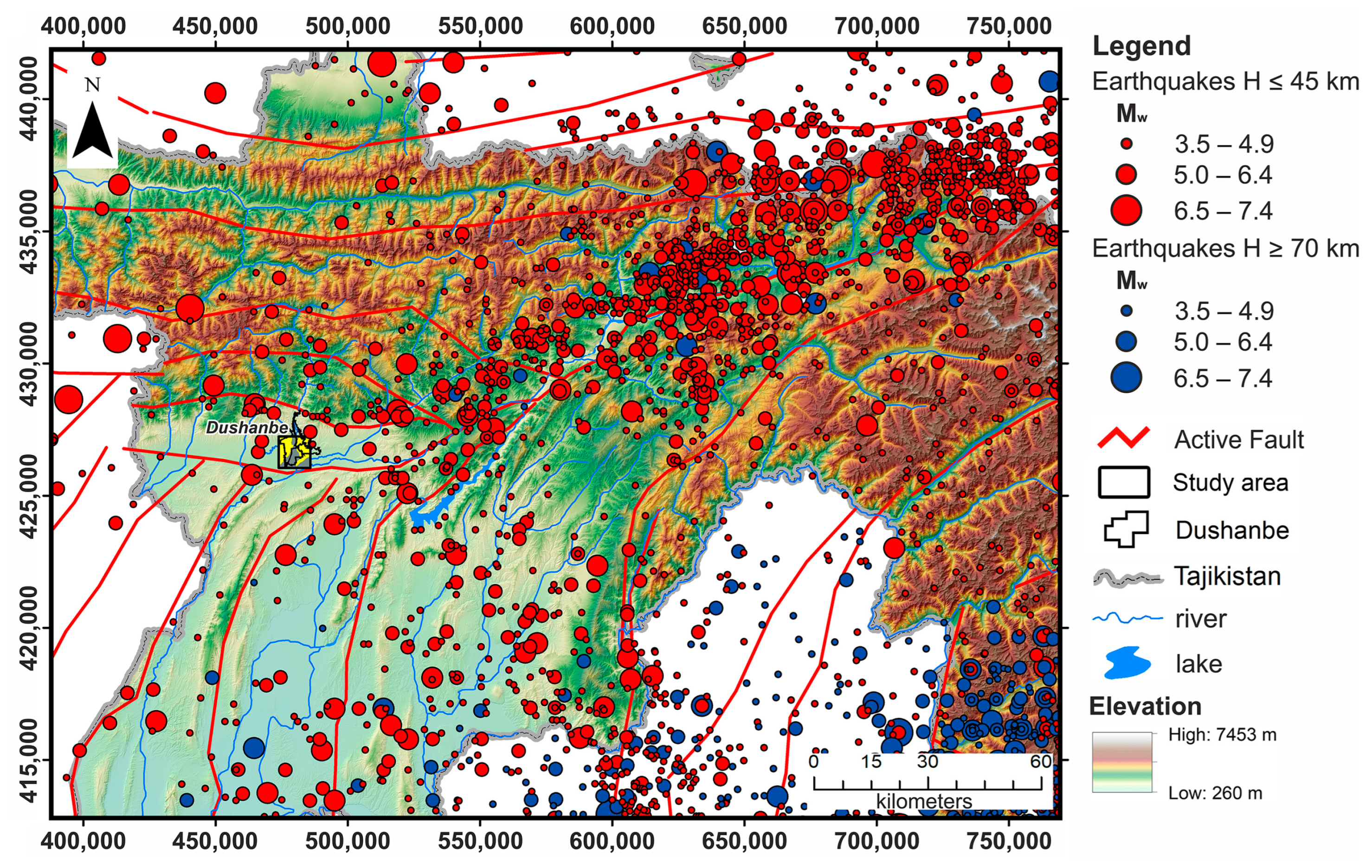
2.1. Seismicity of the Region

The systematic collection of earthquake records in Central Asia and Tajikistan began in 1895. In Tajikistan, the first seismic station was established at the end of 1939 in the capital, then known as Stalinabad till 1961 (now Dushanbe), at the Stalinabad Astronomical Observatory. By 1986, an extensive network of analog seismic stations had been established in Tajikistan, allowing for reliable data collection on seismic events both within the republic and beyond its borders. The map of earthquake epicenters in Tajikistan demonstrates both shallow (depth ≤ 45 km) and deep focal (depth ≥ 70 km in the Pamir area) earthquakes, providing a clear understanding of seismic activity in the region (Figure 2).
An analysis of all available catalogs, including the Central Asia Seismic Risk Initiative–Earthquake Modelling of Central Asia (CASRI–EMCA; [36,37]), covering the period from 818 CE to the present, was conducted. During this research, some adjustments and clarifications were made. As a result, a catalog of strong and perceptible earthquakes in the Dushanbe–Vaksh area from 1907 to 2015 was compiled, with intensity at the epicenter of more than VI units on the MSK-64 scale [38].
Throughout its history, Dushanbe has frequently faced strong seismic impacts caused by local and regional earthquakes. From 1907 to 2007, around Dushanbe city, 17 earthquakes with magnitudes ranging from 3.7 to 7.4 and epicenter intensities between VI and IX units on the MSK-64 scale were registered (Table 1). These earthquakes were manifested within the city’s limits with intensity from III and VII units on the MSK-64 scale. Specifically, Dushanbe was affected by tremors with intensities of VII–VIII (i.e., “very strong”) units on the MSK-64 scale during the 1907 Karatag earthquake and intensity of VI during the 1952 Stalinabad earthquake. Additionally, the city recorded tremors with intensities of VI–VII (i.e., “strong”) units on four occasions: the 1943 Fayzabad earthquake, the 1949 Khait earthquake, the 1980 Dushanbe earthquake, and the 1989 Hissar earthquake (Table 1; [38,39]).

2.2. Seismic Hazard Affecting Dushanbe City

In this context, assessing urbanized areas’ seismic hazards and vulnerability becomes a priority task for earthquake-prone regions. This paper is focused on the local seismic hazard affecting the capital of Tajikistan, Dushanbe city, located between two active tectonic faults (Figure 1): the Hissar–Kokshaal and the Ilyak–Vaksh [40,41]. As a result, early seismic microzonation maps classified most of the city’s areas as having IX units of intensity (i.e., “destructive”) on the MSK-64 scale [42,43].
Until now, studies of seismic hazards in Tajikistan have used a predominantly qualitative approach to seismic microzonation. The study of the effects of strong earthquakes has significantly influenced the methods of seismic microzonation of Tajikistan, the delineation of seismogenic zones [44], and the microzonation of significant cities, as noted in the studies of Kogan et al. [40].
Early seismic microzonation maps of Dushanbe were developed in 1937 by Tsshoher [45] and in 1948 by Medvedev [46], mainly based on engineering-geological and hydrogeological data. These maps divided the city’s territory into zones with a seismic intensity of VII and VIII units (i.e., “very strong”) according to the MSK–64 scale. In 1953, instrumental data on weak earthquakes created the third seismic microzonation map that identified zones of seismic intensity VIII, IX, and above IX on the MSK–64 scale within Dushanbe [42].
The latest seismic microzonation map, which now serves as the standard, was compiled in 1975 [47]. The Quaternary loess is one of the most common types of deposit in the city and its surroundings, characterized by varying thickness and hydromechanical properties; clays, sands, and gravel are also encountered [48]. Recently, new data on the seismic microzonation of Dushanbe have been obtained, covering not only general geological conditions but also new geophysical data and records from a temporary seismic network [34].

3. Materials and Methods

In modern seismology, collecting high-quality data is crucial for successful research. This project employed advanced methodologies to gather accurate and comprehensive data for subsequent analysis.
Our research is based on a database containing seismic and detailed geological information pertinent to urban areas. The goal is to convert qualitative data into quantitative measures through scientifically grounded numerical models. These models aim to encapsulate the earthquake process, focusing on the “Source”, “Path”, and “Site” components [49,50]. Emphasis is placed on the “Site” component, particularly the geological structure of the urban areas being studied.
Probabilistic seismic hazard assessments inform the components of the “Source” and “Path”. This involves (a) convoluting ground motions from earthquakes at rocky sites with models of local amplification effects and (b) using scenario earthquakes for numerical modeling. However, it’s noted that modern computational resources are often limited for comprehensive two-dimensional dynamic modeling.
In the first part of this project, conducted in Dushanbe during 2019–2020, extensive geological and geophysical data were collected. These data encompass five microtremor array measurements (MAM), nine seismic refraction tomography (SRT), five temporary seismic stations for SSR from earthquake data, 60 borehole data, and 175 measurements of HVSR (Table 2). All these data were integrated and presented on maps within a Geographic Information System (GIS) using a unified reference system, as detailed in the first part of our project by Hakimov et al. [34].

3.1. Geophysical Surveys in Dushanbe

Current data from field studies were applied to confirm the modeling results of the Dushanbe area. In the project’s initial phase, a dataset for the seismic microzonation of Dushanbe was formed and processed (details in Hakimov et al. [34]; Table 2).
Within the scope of this research, borehole data were expanded. New measurement data were combined with lithological settings, geological profiles, and information from 60 borehole loggings supplemented by records of 20 other boreholes. All borehole information was collected in the studied area of the city of Dushanbe based on materials provided by the Head Institute of Engineering and Technical Surveys of the State Construction Committee of Tajikistan (HIETSCCT; [51]; Table 2 and Figure 3a).
Below, we summarize the results of seismic and seismological surveys, which are considered the most relevant input data for the 3D geomodel study and 2D dynamic numerical modeling, as described in Section 3.5 and Section 3.6 of this paper, respectively.

3.2. Summary of Ambient Noise Measurements

Ambient noise measurements at a single station were processed using the HVSR method. Based on the data obtained using a mobile single station, we developed maps of changes in the characteristics of identified resonance frequency peaks in the study area (Figure 4).
All measurements of the ground motion characteristics of the medium in this area were carried out with a maximum interval of about 500 m between the nearest points. Based on the HVSR measurement data, several ground motion parameters in the study area were presented: (a) the main resonance frequency (f0), (b) the amplitude of the main peak (A0), and (c) the polarization of ambient noise. Figure 4 illustrates these parameters in selected HVSR recordings in the target areas of Dushanbe city, indicating the fundamental resonance frequency (Figure 4a), the amplitude of the main peak (Figure 4b), the polarization of the ambient noise (Figure 4c), and HVRS plots for specific parts of the study area (Figure 4d). Here, the fundamental resonance frequency is the lowest frequency with a relatively distinct peak.
By interpolation between individual measurement sites, the main resonance frequencies of sediments in the study area were determined (Figure 4a). Practically, the entire territory is characterized by frequencies well below 2 Hz. The resonance frequency is higher only in the areas near the city center, especially in the W and E parts. In this part of the study area, the thickness of the loess decreases rapidly, and gravels are exposed (Figure 4c). As indicated in the work of Hakimov et al. [34], clear HVSR peaks, i.e., significant impedance contrast, are observed between loess layers and bedrock in the E and W parts of the study area. Flat HVSR curves and low amplitude peaks predominate in the S and N areas along the middle of the site, where the surface consists of thick gravel deposits (Figure 4c), consistent with the data from Pilz et al. [11] and Hakimov et al. [34].
Figure 4c presents a map showing the polarization of ground motion at identified resonant peaks. In this map, HVSR findings are depicted using diamond shapes, where the diamond’s color indicates the frequency, its size illustrates the corresponding amplitude, and the direction of its longer diagonal indicates the preferred shaking azimuth. It is noticeable that ground motion polarizations vary considerably on loess deposits, particularly those to the W and E of the study area adjacent to the Adyr hills (Figure 4c). Therefore, it seems that the polarization of ground motion at these resonant frequencies is influenced by the slope orientation of the Adyr hills, especially near the W and E sides of the hills. All identified HVSR peaks along the Adyr hills, ranging between 0.4 and 2 Hz (as established from the SSR data, see Section 4.1), are presumably the result of resonance within the loess layer. Nonetheless, at azimuths generally parallel to the Adyr hills, these peaks are characterized by a minor and more localized morphological impact, as detailed in Figure 4c.
For a more detailed examination and to view a map across the city and corresponding HVSR graphs, reference to the work of Hakimov et al. [34] is recommended. This paper focuses on applying the HVSR method to map the characteristics of the site effects, constructing a 3D geomodel based on HVSR studies of the site effects, and comparing the HVSR results with the results of numerical dynamic modeling.

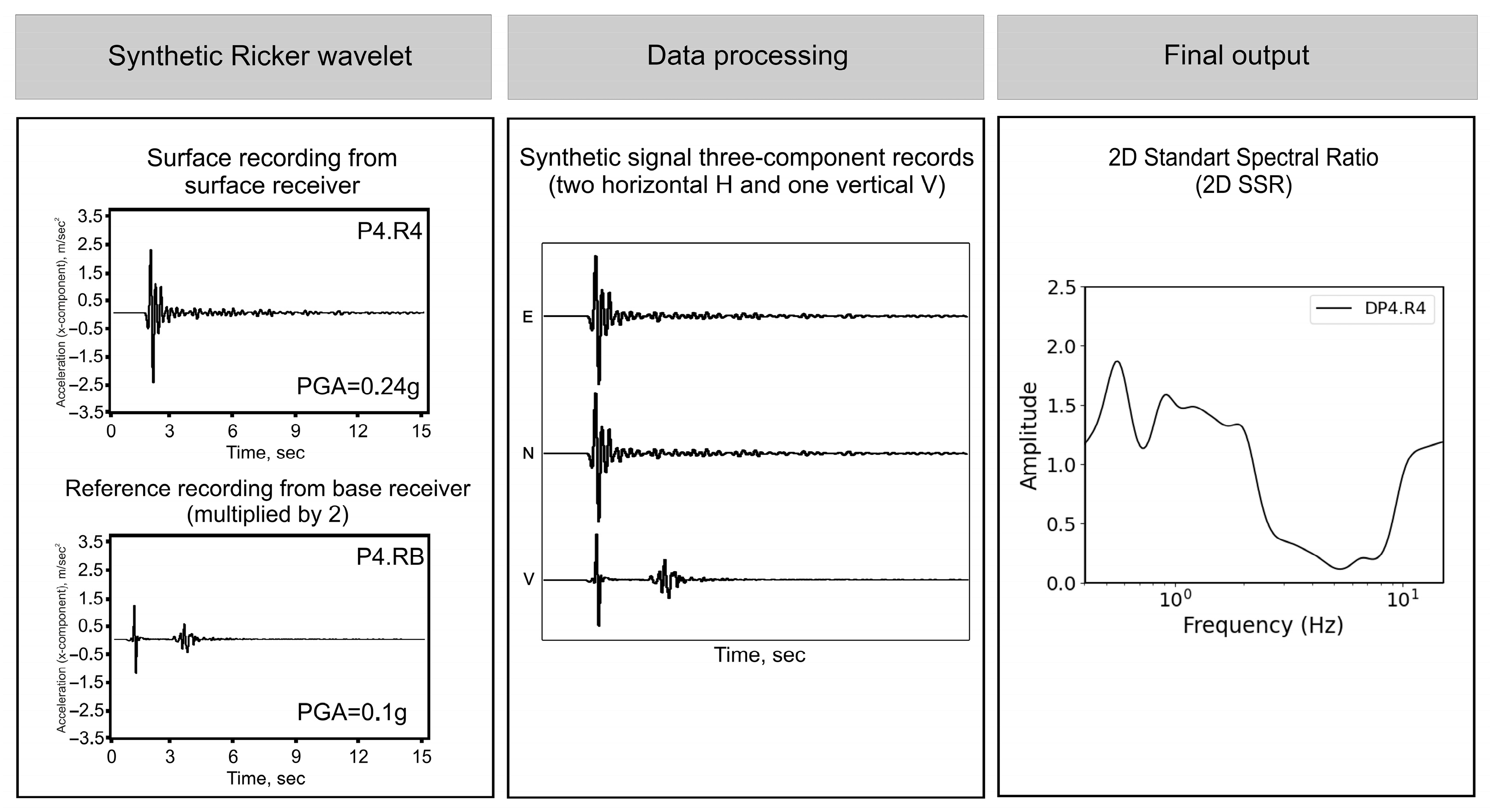
3.3. Earthquake Records and SSR Method

The site response is typically determined using the SSR method, comparing recordings at the analyzed site with those from a nearby base station. It is assumed that recordings from the base site (usually a station located on open hard bedrock) include the same effects from the source and propagation as recordings from other sites. Thus, the spectral ratio can provide information about the site response [34].
Using the earthquake data from our project (see Hakimov et al. [34]), in this study, we additionally utilized stations that are located within the study area (Figure 3a; Table 3) and recalculated the SSR data using station BAV as the reference station relative to other stations (BB2, BB0, and BAU).
For the analysis of the SSR curve at the BAV station (E and N components; Figure 5(a1)) as a reference, we used the Djerino station (DZET), which is located on the outcrops of Paleozoic rock (granite), approximately 14 km N of the city (Hakimov et al. [34]). As expected, no clear peak can be distinguished on the SSR (E and N components; Figure 5(a1)) and NHVSR curve, although the station has flat curves with a peak at low frequencies (0.8–2 Hz), indicating that the BAV station is located on a denser layer of gravel (Figure 5(a2)). In addition, the EHVSR curve shows slightly more amplification at frequencies of 3–5 Hz than the NHVSR curve (Figure 5(a3)).
The choice of reference station for the study area was simple as the HVSR results at station BAV showed a flat peak; this indicates its suitability as a reference station for SSR. It is essential to highlight that the BAV station is not a perfect reference station but rather a better option in the study area compared to other stations (BB2, BB0, and BAU). As indicated in the study by Hakimov et al. [34], the BAV station is located on consolidated alluvial deposits (Figure 3a).
S-wave windows were defined to assess the SSR curves from the five selected earthquakes, and the Fourier amplitude spectrum (FAS) was calculated for each component using Geopsy software (version 3.4.2; [52]). For each component of S-waves extracted, S-wave windows were taken from selected earthquakes with a taper of 5%, with the window duration based on the most extended temporal duration of the S-waves. Fast Fourier transform was computed, and a smoothing parameter of 40 by the Konno and Ohmachi [53] function was applied to the Fourier spectra. Then, the ratio between the Fourier spectrum of the target site and that of the reference site was executed component by component. The average of the SSR of all the selected earthquakes was finally determined for each station. Only N and E components were considered in the SSR calculations.
The corresponding SSR curves are shown in Figure 5(a1–d1). Their root-mean-square value (Havg) was calculated for all horizontal elements. This parameter determined the HVSR and EHVSR coefficients for combined horizontal components. A review of various methods for combining horizontal spectra can be found in the studies of Albarello and Lunedei [54] and Fäh et al. [55]. These studies also confirm using the quadratic mean in calculating the average spectral ratio. The HVSR curves related to earthquakes (EHVSR; Figure 5(a2–d2)) were determined for each station. Also, HVSR time interval curves that do not correspond to earthquakes were compiled, representing HVSR data related to noise (NHVSR; Figure 5(a3–d3)).

3.4. Microtremor Array Measurements and Seismic Refraction Tomography for the Vs30 Distribution Map

Ambient noise measurements are successfully used for 2D and 3D seismic characterization of subsurface areas, allowing the determination of shear wave velocities (Vs) distribution in underground layers [56,57]. This passive method is particularly suitable for assessing site effects and subsequent seismic hazard analysis [16,58].
According to the MAM and SRT results obtained in the studies by Pilz et al. [11] and Hakimov et al. [34], the lowest Vs (200–250 m/s) and Vp (400–550 m/s) were measured in the NW and NE parts of the city where loess deposits are observed, especially in the E part where the thickness of loess deposits is 80–100 m and the lowest velocities are observed. Higher Vs (400–550 m/s) and Vp (800–1150 m/s) are observed in the city’s N, SW, SE, and center (Figure 6b). These velocities may correspond to a mixed loess–gravel layer, increasing to a gravel–sandstone layer. The highest values of Vs = 550 m/s and Vp = 1150 m/s are observed in the N and are obtained at a depth of 5–8 m, where the gravel layer transitions to the sandstone layer (Figure 6b).
The average shear wave velocity in the upper 30 m of ground (Vs30) was calculated to assess the study area’s seismic stability and ground condition characteristics. This parameter is crucial in seismic microzonation and is widely used in engineering geology and seismology.
Using data from previous studies, SRT, and MAM profiles, we constructed the Vs30 map shown in Figure 6b. The Quaternary sediment was divided into layers, each characterized by a different velocity Vs. Vs30 was calculated according to the recommendations of the National Earthquake Hazards Reduction Program (NEHRP; [59]) and is determined by the following equation:
V s 30 = 30 i = 1 n ( h i / V s i )
where Vs30 is the average shear wave velocity in the upper 30 m of sediment, hi is the thickness of the i-th sediment layer within the 30 m, Vsi is the shear wave velocity in each layer, and n is the total number of layers within the 30 m depth.

3.5. Three-Dimensional Geomodeling

The term “geomodel” refers to a model representing geoscientific data in a 3D environment; thus, we integrated geographic, geological, and geophysical data related to the study site. The main advantage of using 3D geomodeling software, such as Leapfrog Works (version 2021, 2.5), over 2D GIS software is that a single model can simultaneously present and visualize many surface and subsurface data. The primary goal of the geomodel created was to understand the subsurface structures in combination with surface data. The geomodel is a necessary preliminary step before creating numerical models. Here, we extracted a 2D section from the Leapfrog Works model, which will be used for 2D dynamic analysis of the influence of ground characteristics on seismic ground motions (see details and results in Section 4.3).

3.6. Two-Dimensional Dynamic Numerical Modeling Methodology

The study focused on modeling ground motions and amplification effects in Dushanbe city, considering several influencing factors. To accurately characterize the mechanical behavior of discontinuous materials, we employed the Distinct Element Method (DEM), integrated within Itasca’s UDEC software (version 2021, 6.37). DEM, initially developed by Cundall [60] for rock mechanics analyses, effectively handles discrete elements or blocks, each defined by unique elastic properties and distinct layer boundaries.
In our study, the UDEC software, which combines DEM with the finite difference (FD) method, was pivotal for conducting the 2D numerical experiments. This integration is particularly advantageous as it allows for precise determination of material deformation within discrete blocks, enhancing the simulation’s fidelity over methods such as 3D interpolation algorithms. While useful for spatial data interpolation, that method only partially accommodates the complex interplay of mechanical behaviors and discontinuities typical in geological substrates.
Moreover, UDEC’s computational efficiency is tailored specifically for 2D simulations, facilitating faster and more resource-efficient analyses compared to 3D models that require higher computational overhead. The capability of UDEC to manage large displacements and rotations within the blocky media structure, as opposed to the smooth interpolations by other methods, was essential. However, in this study, the models were constructed as a continuum. The contacts between surface layers and underlying rock were effectively managed by assigning high cohesion values at the joints, simulating a ‘glued’ interaction, which is crucial for analyzing urban geotechnical environments confined to the elastic range.
Additionally, the application of the Rayleigh damping scheme, following Bathe and Wilson [61], allowed for accurate accounting of energy dissipation mechanisms, such as viscous damping, with free-field conditions maintained along the boundaries. This methodological choice highlights UDEC’s robustness in predictive analysis of seismic ground motion and its superior visualization tools, which are indispensable for presenting complex geotechnical data and deriving insightful conclusions from the modeled mechanical interactions.

3.6.1. The Static Model

Before proceeding with the dynamic modeling process, each model must reach an initial static equilibrium (according to Wolter et al. [62]). Static modeling includes determining the overall structure of the model, model parameters, fluid flow, and boundary conditions (groundwater level values for static and dynamic models in this study were not considered).
The model’s general structure consists of fixed contacts on a 2D plane with diagonally opposite triangular FD zones to enhance elastic flow calculations [63]. The material properties for each layer include Mat1 for the loess layer, Mat2 for gravel, Mat3 for conglomerate, and Mat4 for sandstone. Each contact’s joint material is also specified: one for loess, two for gravel, three for conglomerate, and four for sandstone.
Static modeling establishes the foundation for dynamic analysis by ensuring the model’s initial state of equilibrium. To finalize the static model, boundary conditions are defined within the modeling area. Displacement boundaries are set by limiting velocities for deformed blocks along the x and y axes, preventing displacement at the model’s base and sides. Additionally, a dynamic free field for 1D finite difference calculations is created to simulate seismic wave propagation along the boundaries, facilitating vertical shear wave signal transmission. The node count along the finite difference calculation zone’s edge determines the free field boundaries. Static models are thus characterized by their dimensions, properties, and boundary conditions. An automatic Rayleigh damping coefficient is applied for model stabilization, absorbing vibrational energy. Mechanical calculations continue until static conditions are achieved, indicated by the ratio of unbalanced to applied mechanical forces reaching a set limit (in our case, 1 × 10⁻⁹).

3.6.2. The Dynamic Model

After the completion of static modeling, which is aimed at stabilizing the model, the stage of dynamic modeling follows. This stage is implemented by applying an artificial wave signal to the model base over a set interval. The dynamic response to the load of various model elements is analyzed by studying wave propagation paths and the maximum displacements of the blocks, in our case, layers.
Initially, dynamic boundary conditions are set to facilitate optimal wave propagation in the model area. These include non-reflecting (viscous) boundaries at the model’s base and free field conditions along its sides. This setup predefines initial vertical wave propagation and minimizes seismic wave reflection, as detailed by Wolter et al. [62].
After setting up the dynamic boundary conditions, the model is subjected to dynamic loading through a Ricker wavelet, defined by two primary frequencies: 1.4 and 3.5 Hz. This particular wavelet is frequently used in engineering seismology because it closely mirrors the spectral content of accurate seismic data (as noted by Gholamy and Krienovich [64]). Introduced by Ricker in 1953 [65], the Ricker wavelet is characterized by a specific equation:
A = ( 1 2 π 2 f 2 t 2 ) e π 2 f 2 t 2
where A is the amplitude, f (Hz) is the central frequency (1.4 and 3.5 Hz), and t (sec) is the dynamic time. Figure A1 in Appendix A shows the form of the Ricker wavelet used in this work.
The wavelet propagates from the model’s base, traversing its entirety along the y-axis. The dynamic load’s amplitude and duration vary with the signal. Signal duration is time set and adjusted by scaling peak values with a coefficient. Dynamic modeling and recordings span 15 s to capture all secondary seismic phenomena. This extended duration is crucial, especially for models simulating the cumulative effects of geological conditions and terrain, as these secondary effects may emerge over time.
To confirm the modeling results, 48 synthetic receivers (“history points”) were strategically placed around the model’s perimeter on its free surface for each of the six profiles. A reference receiver is situated at the model base, nearly −1000 m deep, with the highest point at 1100 m (Figure 3b). These “history points” monitor a range of parameters over time, such as displacement, velocity, and acceleration in x and y directions. They continuously record synthetic signals on the surface during the modeling process, capturing velocity and acceleration data both at the model’s base and its surface.
FD zones are key points in dynamic modeling, where their size affects the velocity of computations and the transmission of high-frequency seismic signals. Large FD zones velocity up computations but are less efficient at transmitting high frequencies, while smaller zones do the opposite. An ideal FD zone size that balances velocity and signal efficiency was proposed by Kuhlemeyer and Lismer [66]. They suggested that the FD zone size (∆l) should be approximately one-tenth of the wavelength of the highest frequency (λ) in the input shear wave, according to the equation:
l λ 10 l V s 10 × f
where Vs (m/s) is the shear wave velocity, and f (Hz) is the modeled frequency. In models using Mat1 (loess) with Vs = 320 m/s and an upper frequency of 8 Hz, ∆l is about 5 m. Larger FD zones are used in the lower parts of the model to speed up seismic energy calculations. Accurate alignment of nodes between neighboring zones is critical to avoid artificial reflections, especially at contacts between zones of different sizes. Although computationally expensive, this alignment is often necessary for accurate modeling (see details in Section 4.4).

4. Results

4.1. SSR Results

Station BB0, positioned on the side opposite BAU, is situated atop a slim loess layer (5–10 m), beneath which lies a layer of gravel, as depicted in Figure 3a. Consequently, its peak pattern resembles station BAV, established on a gravel base. The SSR graphs illustrate modest amplitude peaks within the 0.6–1 Hz frequency range, reaching amplitudes between 2 and 4. Furthermore, these graphs show a slight amplitude rise in the 4–6 Hz frequency spectrum. This increase is more pronounced in the EHVSR curve, exhibiting amplitudes of 3–6. On the NHVSR curve, a subtle but distinct peak at 5.8 Hz with an amplitude of 3 indicates its location above a thin layer of loess, as shown in Figure 5(b1–b3). The correlation of these data with data from nearby boreholes and geologic cross-sections confirms the existence of a surface layer of loess above the gravel layers, as shown in Figure 3a.
The data from Station BAU (Figure 5(c1–c3)) show similar peaks from 0.5 to 1 Hz, accompanied by a clear peak between 3 and 5 Hz, with amplitudes ranging between 4 to 5. This is particularly evident in the SSR (E and N components) and EHVSR (Figure 5(c1,c2)). Additionally, the NHVSR data indicate that a slight bump can be observed at the lower-frequency range of 0.5–1 Hz and a clear peak around 4.5 Hz. The low-frequency peaks (0.5–1 Hz) observed in the SSR curves (E and N components; Figure 5(c1)) and in the EHVSR (Figure 5(c2)) are likely related to a deeper and more compact layer (sandstone or conglomerate), identified as bedrock.
Station BB2, located in the W part of the city with a thick loess layer, exhibits numerous peaks at lower frequencies (0.4–6 Hz), as shown in Figure 5(d1–d3). The N and E components of the SSR curves show several peaks at 0.4 to 4 Hz range, having amplitudes ranging from 4 to 9 (Figure 5(d1)). In the 1.5–6 Hz frequency band, peaks of lower amplitude are observed on the EHVSR (Figure 5(d2)). In addition, a clear peak at 1.5 Hz is noticeable on the NHVSR curve (Figure 5(d3)). Analysis of borehole data around the station indicates that the thickness of the loess layer is 40–45 m, increasing near the Adyr hills and including sandstone layers below (profile DP1; Figure 3b).
In summary, there is a notable consistency in the form and position of the fundamental resonant frequency identified by the SSR, EHVSR, and NHVSR curves. The spectral coefficients of EHVSR and SSR (E and N components) are similar in shape and magnitude, with the minor amplification observed at the BAV station attributed to topographical effects not significantly altering the outcomes. Stations BB2 and BAU on a thin loess layer typically exhibit higher amplification levels. Reliable responses on EHVSR and SSR sites can generally only be obtained when earthquakes are distributed around the stations at various distances. A strong impedance contrast is the primary cause of the elevated amplitudes at several sites. This assertion is reinforced by examining the site’s ground conditions and aligns with the research findings of Pilz et al. [11] and Hakimov et al. [34].
The extent of amplification reveals variations in the spectral ratios of NHVSR and EHVSR—earthquake data typically exhibit higher amplification levels than NHVSR across broader frequency ranges. NHVSR tends to show lesser amplification, particularly at lower frequencies, and around 1 Hz, the amplification ratio of SSR to NHVSR falls below one. At some of the stations (BAV, BB2 and BAU) located over thicker sedimentary rock layers, noticeable peaks correspond to higher harmonics on both EHVSR and SSR (E and N components) curves, where amplification often is greater than 3. Given that NHVSR is commonly used to gauge only the fundamental resonant frequency (or offer amplification in a limited frequency band around it), it is likely to underestimate amplification at frequencies above this fundamental frequency significantly. Consequently, the amplification ratio of SSR (E and N components) to NHVSR is anticipated to fluctuate with frequency and vary among different stations, depending on the location of the peak associated with the fundamental frequency.

4.2. Maps of the Distribution of Site Effect Inferred from HVSR Results in the Study Area

A map illustrating the site effects on the study area can be seen in Figure 6a. As part of this study area’s initial approach to seismic microzonation, we first performed interpolating values: fundamental resonance frequencies of HVSR (the most pronounced low-frequency peak) and corresponding peak amplitudes (Figure 4).
The first two maps in Figure 4, detailing interpolated resonant frequencies and peak amplitudes, were combined to produce a map showing the intensity of the site effects (Figure 6a). This map identifies areas with pronounced site effects, characterized primarily by elevated peak HVSR amplitudes (greater than 3) and fundamental resonant frequencies important for earthquake engineering (below 5 Hz). Areas that exhibit these combined features are highlighted in red in the HVSR distribution map for site effect, as shown in Figure 6a and distribution site effects on 3D geomodel shown in Figure 6b. Notably, these areas are concentrated in two main regions: a larger area in the E part and a smaller area in the W part. It is important to note that these summary data do not account for topographic effects (especially at low frequencies) and focus solely on site effects potentially due to ground amplification.
Figure 6 shows the “HVSR site effect” distribution map (Figure 6a) together with the Vs30 distribution map (Figure 6b). Low Vs30 values characterize sites with very strong site effects. Both very strong and strong site effects (marked in red and gold colors in Figure 6a) are observed in the Adyr hills area in the NW and NE, where loess cover over compacted gravel and sandstone layers is present. It is also observed that Vs30 values increase in the central, SW, and SE parts of the study area. The site effect distribution map shows two main zones: the first zone in the W and SW shows moderate to slight site effects (marked in yellow and light green colors in Figure 6a). The second zone in the NE and SE similarly shows a transition from moderate to slight site effects. The SW, SE, and central parts of the city show very slight and no site effects (marked in blue and light blue colors in Figure 6a). Similarly, these areas are highlighted by high Vs30 values on the Vs30 distribution map (Figure 6b).

4.3. Three-Dimensional Geological Model Development

The integration of various data sources is critical to creating a cohesive and objective picture of the geological structure. All collected data were combined to create a uniform 3D geomodel of 12 × 12 km2, which served as the basis for further research.
Based on data from 100 HVSR, four SRT, three MAM measurements, and 80 boreholes, a 3D geomodel of the Dushanbe city area measuring 12 × 12 km2 was created using Leapfrog Works software (Figure 7b,c). At each point where HVSR measurements were conducted, the thickness of surface layers was determined using the following equation for HVSR data:
h = V s 30 4 f 0 ,
where h is the thickness of the layer, and f0 represents the determined resonance frequency. Also, the second and third peaks of HVSR were calibrated, considering data from nearby boreholes. For a more precise distribution of values, the first loess layer was divided into W and E parts, excluding the central part from N to S, where gravel predominates, based on borehole data and geophysical measurements.
In this case, the subsurface model geometry is reconstructed using a digital geologic map and a 3D geologic model. Figure 7 shows the geologic map and 3D geologic model scale covering the central part of the study area. The collected data include geologic cross-sections, borehole data, and geophysical information. Extensive field surveys conducted early in the project (see details in Hakimov et al. [34]) facilitated the accurate determination of contact points and provided an accurate representation of the structural arrangement of the geologic layers. Thus, the resulting 3D geomodel represents a geological structure consisting of four layers: sandstone (brown), conglomerate (pink), gravel (gray), and loess (yellow).

4.4. Two-Dimensional Dynamic Numerical Modeling Results

4.4.1. Two-Dimensional Dynamic Numerical Modeling Applied to Six Profiles

The models use three contact types to represent the underground structure geometry: material, dividing, and sub-division contacts, as demonstrated in the DP5 profile model in Figure 8. Material contacts separate different materials, used only in combined topographic-geological model, while dividing contacts segment the model into areas with varying FD zone edge lengths. For example, the upper model parts use 5 m and 10 m edge-length zones. In contrast, the lower parts have double-sized zones, with these dividing contacts being horizontal and positioned 20 to 300 m below the surface (Figure 8b). Sub-division contacts further split large blocks into smaller sub-blocks due to UDEC code processing limits, requiring substantial memory and potentially exceeding standard computer capacities [63]. These contacts are aligned horizontally or vertically for effective zoning.
Node velocities in the model were adjusted using an automatic Rayleigh damping coefficient to optimize energy dissipation and reproduce the system’s natural behavior. The model employs geotechnical parameters characterizing block material and joint properties, including Young’s modulus (E), bulk modulus (K), shear modulus (G), dry density (ρ), Poisson’s ratio (ν), joint standard and shear stiffness (jkn and jks), joint tensile strength (jtens), and cohesive forces (jcoh) at contacts (Table 4). K and G values were derived from P- and S-wave velocities and analyzed from seismic profiles using wave equations. Elastic properties, such as Vs values and densities, which ranged from 1900 to 2400 kg/m³, were based on the findings of Kapylov [48] and Hakimov et al. [34]. Thus, the contacts between surface layers and other blocks were reinforced by assigning high values to the last parameters. They were set at values (104 kg/m3), (104 GPa), and (104 MPa), respectively.
Based on borehole data and geophysical surveys, we identified four geological layers in the Dushanbe area, as mentioned above. Figure 8a shows how the sequence of geologic formations in the target area serves as a basis for defining the modeled materials. Thus, all formations are summarized through the four material types. Table 4 summarizes the geotechnical and dynamic property values used in the subsequent dynamic modeling. According to the values of shear wave velocity (Vs) and borehole data, the soft material type is represented as Mat1 (loess). The Mat2 layer gravel is classified as a hard material, Mat3 (conglomerate) is the second hardest material, and Mat4 (sandstone) represents the hardest material in the modeled sequence. The characteristic moduli were calculated from the measured seismic velocities (Vp, Vs) and design density (ρ) of the material according to the equations provided in Appendix A.

4.4.2. Two-Dimensional Dynamic Numerical Model Processing

Ricker wavelets were recorded using 48 synthetic receivers placed on the surface of each profile and six synthetic reference receivers at the base of each profile, allowing for the assessment of surface effects concerning the modeled subsurface conditions. The SSR was calculated for the 48 synthetic surface receivers. We employed this method to analyze the spectral ratios of the modeled data. The Geopsy software (version 3.4.2; [52]) was used to study spectral amplification. As noted earlier, the main focus in Geopsy is on determining object characteristics through the analysis of ambient noise. One of the seismic noise analysis tools in Geopsy is based on the HVSR method.
This method was applied to investigate the spectral properties of the modeled data. All surface acceleration records of the x-component were compared with the corresponding model base data (obtained from the reference receiver P4.RB). These reference receivers from the model’s base were then doubled and subjected to a filtering process. A synthetic dataset consisting of three-component records was created for each receiver under consideration, as shown in Figure 9 on the example of synthetic receiver P4.R4 of profile DP4. In this dataset, the surface receivers cover records from the reference receiver, replacing both horizontal and vertical components. This synthesized dataset is subsequently analyzed using the HVRS method schematically illustrated in Figure 9. Fourier spectra are computed for all recordings, similar to the HVSR analysis process. The spectral amplitudes of the surface recordings are then divided by the reference amplitudes, similar to the HVSR separation method. This process results in a spectral ratio curve for each surface receiver, as shown in Figure 9.
Similar to the provided example, the resulting curve effectively depicts the spectral scenario of deamplification or amplification. Consequently, the curve shown in Figure 9 indicates that the surface “history” experiences amplification in three distinct spectral ranges relative to the reference recordings. The most pronounced amplification, exceedingly almost 2, is observed at a frequency of around 0.5 Hz. On the other hand, deamplification in the spectrum is noted in two frequency bands, with the most significant deamplification observed at a frequency of 1 Hz. The insights from these spectral studies are then utilized in our analysis to establish a correlation between spectral amplification and the HVSR and SSR methodologies.

4.5. Results of 2D Dynamic Numerical Models: 2D SSR Analysis

Using 2D dynamic numerical models, it was established that the propagation of seismic waves in the study area of Dushanbe could vary significantly depending on lithological and topographical conditions.
In this section, we demonstrate the results of 2D SSR analysis, which were calculated for six profiles in the study area in Dushanbe using the Ricker wavelet. Data were collected from 48 synthetic surface receivers and six reference receivers. A comparison of SSR (average of E and N components), EHVSR, and HVSR data was also conducted with results obtained from Hakimov et al. [34] and with the results of 2D SSR from synthetic receivers (Figure 10).
The analysis of 2D SSR revealed a series of peak frequencies within the ranges of 0.6–2 Hz, 3–4 Hz, and 5–6 Hz. The most notable minimum peaks, identified at 0.6–0.7 Hz, are regularly observed with varying amplitudes on most 2D SSR curves. Of particular interest is comparing these SSR (average of E and N components), EHVSR, and HVSR data with results obtained from previous studies by Hakimov et al. [34], where similar peak frequencies were found. This low-frequency peak is consistent with measurements taken at stations BAV, BAU, BB0, and BB2, according to SSR (E and N components), EHVSR, and NHVSR (Figure 5), where overall analysis indicated the presence of several moderate peaks in the ranges of 0.6–2 and 3–5 Hz across all profiles of the study area (Figure 10).
Topographic amplification is predominantly observed with coefficients between 1 and 2 in the W and E parts of the city, characterized by a thick layer of loess (Figure 7a). In these areas, according to SSR (average of E and N components), EHVSR, and HVSR data, an increase in amplitude of four times or more was recorded (Figure 5). Historical data show that in the NW and NE of the city, there are thick surface loess layers, reaching a depth of more than 40 m, which is confirmed by studies by Kopylov [48], Pilz et al. [11], and Hakimov et al. [34].

4.5.1. Comparison of Results in the SW to the Central Part of the Study Area on Gravels

The DP2 and DP6 profiles are located on gravels extending from N to S (DP2) and from W to E (DP6), as shown in Figure 7a. The results obtained at the DA4 and DA3 arrays located on gravel show the presence of two distinct sedimentary layers consistent with the Vs profiles (DA4 and DA3; Figure S1 reported in the Supplementary Materials). The upper layer, characterized by Vs values in the range of 400–700 m/s, suggests gravel deposits, while the deeper layer, with Vs values in the range of 1200–1250 m/s, indicates more complex rock formations. Specifically, for DA4, the Vs 1200–1250 m/s range starts at a depth of 65 m, while for DA3, it starts below 55 m, as shown in Figure S1 reported in the Supplementary Materials. In addition, this SW trend of deepening of the upper conglomerate layer is supported by cross-sections of DP2 and DP6 profiles, as shown in Figure 3b.
Seismic response at station BAV in the SW shows minimal seismic amplification, making it the reference for SSR calculations (Figure 5(a1–a3)). Comparisons with DP2.R6 and HVSR peaks (D144 and D146; Figure 10) near BAV show flat curves with peaks at low (0.8–1 Hz) and high (6–8 Hz) frequencies on dense gravel layers (Figure 3b). BAV’s SSR (E and N components) curves lack high-frequency peaks, except for a 3.9 Hz peak on its EHVSR curve (Figure 5(a1–a3)). The synthetic receiver DP2.R6 shows a 4.9 Hz peak with a lower amplitude (Figure 10).
Similar results are evident in the N part of the study area, where the DP2 and DP4 models intersect at the gravel area in the center of the study area (Figure 7a). Two-dimensional SSR data obtained from the DP2.R1 and DP4.R4 receivers show coincident low-frequency peaks (0.6 Hz) with relatively low amplitude. When comparing these data with HVSR results (D72 and D74; Figure 10), the low-frequency peaks are absent, but high-frequency peaks (3–9 Hz) with low amplitude (<2) are present, which may indicate the influence of the river channel on these high-frequency peaks.
All receivers on gravel deposits (DP3.R8, DP6.R3, DP6.R7) show no pronounced SSR peaks (Figure 10). DP6.R7’s 2D SSR data correlate with HVSR at D175, showing a peak at 4–5 Hz. DP6.R3’s results match DP6.R7 at low (0.6 Hz) and high (4–5 Hz) frequencies but differ from HVSR data (D147, D148; Figure 10), suggesting local topographical influences on seismic response.

4.5.2. Comparison of Results in the NW, NE, and SE Part of the Study Area on Loess

In the NW study area, synthetic receivers DP1.R1, DP1.R2, and DP4.R1, along with seismic station BB2 on loess deposits, show high amplification factors (Figure 10). SSR data from BB2 and these receivers reveal distinct peaks at 1–1.5 Hz, supported by HVSR measurements (D165; Figure 10). DP1.R2, located on a thinner loess layer, shows a 2.5 Hz peak in SSR and HVSR data (D69; Figure 10), indicating decreasing loess thickness from N to S.
The SRT profiles (DSP3, DSP4, DSP5; Figure S1 reported in the Supplementary Materials) in the NW study area demonstrate a consistent decrease in surface longitudinal wave velocity, aligning with loess presence [34]. Borehole data and DP1 geological cross-sections confirm loess thickness reduction from N to S. At depths over 30 m, where loess turns to gravel, longitudinal wave velocity increases. This is further affirmed by MAM shear wave velocities (DA5; Figure S1 reported in the Supplementary Materials), revealing a decrease in Vs up to 45 m, associated with loess, and an increase below, indicating a shift to a gravel layer on top of bedrock at 70 m.
In this direction, we also observe seismic station BB0 and synthetic receiver DP5.R3 of model DP5 (SW to NE orientation), both located on a thin loess layer (5–10 m) overlaid by gravel (Figure 10), showing similar peak patterns to station BAV and receiver DP2.R6 on gravel. BB0’s SSR (E and N components) curves exhibit peaks at 0.6–1 Hz (amplitude 2–4; Figure 5(b1–b3)) and a modest increase at 4–6 Hz, more pronounced on the EHVSR curve (amplitude 3–5; Figure 5(b2)). The NHVSR curve indicates a small peak at 6 Hz (amplitude 3), indicating its location on a thin loess layer (Figure 5(b1–b3)). Compared with DP5.R3 (2D SSR) data, it shows similar frequency peaks in HVSR (D77, D82; Figure 10) near these points, with a peak at 0.9–1 Hz (lower amplitude) and distinct peaks at 6–10 Hz. HVSR (D77) closely matches DP5.R3 data, both on thin loess (<10 m), while D82 indicates an even thinner layer (<5 m), confirmed by the HVSR frequency of 10 Hz and borehole data and DP5’s profile cross-section (Figure 3b).
Data from DP2.R3 and HVSR receivers (D62 and D76; Figure 10) located near the thin loess layer show low-frequency peaks and a distinct peak at 6 Hz, consistent with the D76 results, while D62 shows a peak at 9 Hz in an even thinner loess layer (<5 m). In the NE and SE of Dushanbe, the overlapping models DP3 and DP4 (DP3.R1 and DP4.R6) and DP3 and DP5 (DP3.R3 and DP5.R6) show low-frequency peaks and significant amplification at 4–4.5 Hz in the area near the BAU seismic station, indicating impedance contrast between loess and gravel (Figure 10). The BAV station located on gravel contrasts with BAU by the absence of high-frequency peaks, indicating different amplitudes of the data for SSR and EHVSR but similar depth structures. Near BAU, the data for DP5.R5 and HVSR (D161) show low and distinct peaks at 3–4.5 Hz, reflecting similar thickness of loess. DP3 overlaps with DP4 and DP5, showing consistent low-frequency peaks and high-frequency similarities at 3 Hz, indicating similar loess layers (Figure 10).
DP5.R8, located on a thick loess layer in E, shows a distinct 1 Hz peak in the SSR data, possibly influenced by topographic amplification as suggested by nearby HVSR data (D127, D128; Figure 10). We discuss these topographic effects in more detail in the Section 5.

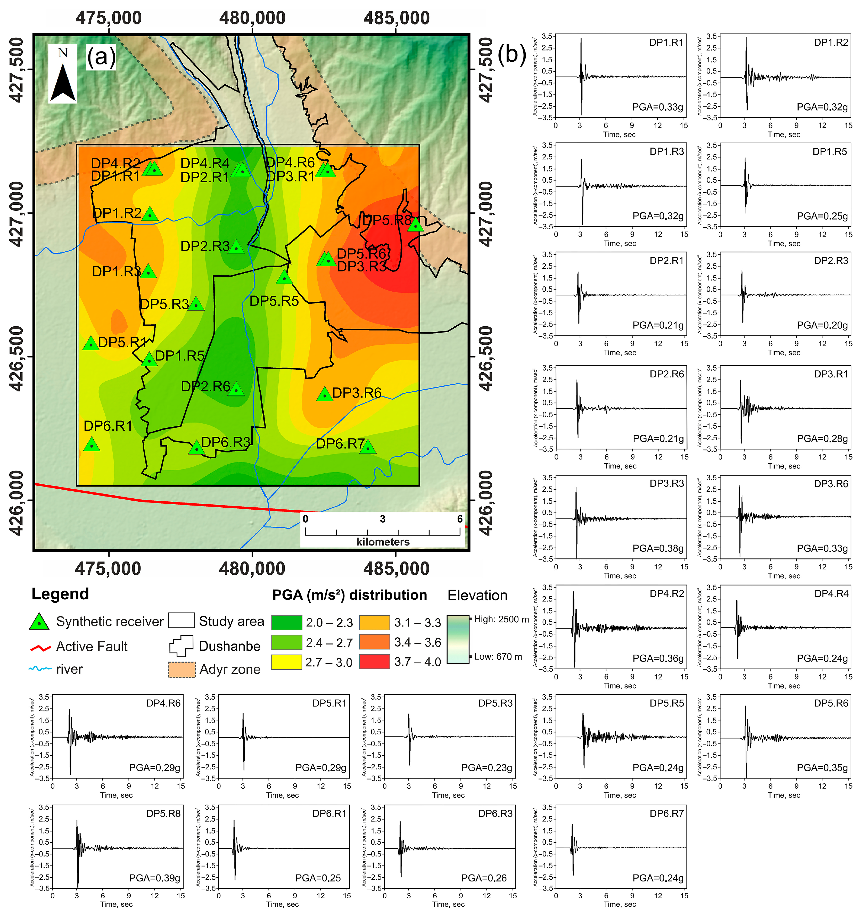
4.6. PGA Distribution Inferred from 2D Dynamic Numerical Simulations

Shear waves propagate more smoothly from hard to softer materials, but as they travel from softer to harder materials, they encounter reflection or refraction due to changes in shear wave velocity impedance (Vs). This causes seismic energy to be intensified in materials with lower Vs values due to geologic factors, which are accompanied by prolonged seismic shaking and enhanced peak ground motion. The DP5 profile, as shown in Figure S2 reported in the Supplementary Materials, illustrates these dynamics. In this model, as shown in Table 4, loess (Mat1) has the lowest Vs, followed by gravel (Mat2), conglomerates (Mat3), and sandstone (Mat4) have the highest Vs. This arrangement of Mat1 and Mat2 materials favors the capture of seismic energy. Although the energy in Mat3 and Mat4 materials is largely dissipated, seismic shaking in Mat1 is much more prominent. The PGA values in Mat1 are 2–3 times higher than in the other materials.
Figure S2, reported in the Supplementary Materials, shows PGA data for eight surfaces and one reference receiver on the DP5 profile, analyzing PGA amplification and duration of seismic shaking. The analysis focuses on x-component acceleration for DP5 surface receivers, using P5.RB at the model base as a reference. Surface receivers in Mat1 experience 3–4-times-longer seismic motion than those in Mat2, except for P5.R5, which shows significant secondary shaking due to its location at the Mat2 and Mat3 boundary. The highest PGA amplification is observed in Mat1, with lower values in the more complex Mat2. This variation is linked to material structural characteristics, where thinner layers lead to shorter shock durations and potential amplification from wave focusing. Topographic effects further enhance PGA at P5.R7 and P5.R8, located on hilltops with thick loess deposits.
Figure 11 shows Ricker wavelet calculations for PGA distribution across Dushanbe city models, indicating higher accelerations on loess deposits than gravel (Figure 11b). This suggests a tendency for more significant loess acceleration than gravel.
Higher PGA values are observed on loess deposits in the city’s NW and NE parts, with lower values in central gravel areas. This highlights the accurate simulation of vertical variations in dynamic geotechnical properties. Specifically, the NE Adyr hills receiver DP5.R8 shows the highest PGA (0.39 g), and the NW loess areas (receivers DP1.R1 and DP4.R2) also exhibit high values (0.36 g). In contrast, central gravel areas (receivers DP2.R1 and DP4.R4) display lower PGAs (0.21 g and 0.24 g, respectively).
In the NE, the intersection of models DP3 and DP4 at receivers DP3.R1 and DP4.R6, both on loess deposits, shows consistent PGA values of 0.33 g, reflecting uniform loess thickness as verified by nearby geological data. PGA analysis in Dushanbe indicates that loess thickness and topography affect amplification, notably in the Adyr hills, where sharp relief changes significantly increase PGA in the NE and NW. The complex PGA distribution in gravel areas also points to topographical impacts, with increases observed mainly in the E part of the study area. The significant PGA amplification in topographically varied regions like the Adyr hills suggests the influence of wave reflections. Despite lower absolute PGA values in these regions, the importance of detailed topographical analysis in seismic hazard assessments for Dushanbe is underscored. The forthcoming Section 5 will juxtapose these observations with historical earthquake data, aiming to deepen our understanding of seismic activity and assess the effectiveness of seismic risk analysis models.

5. Discussion

5.1. Analysis of the Site and Topographic Effects and Their Impact on the NE and SE Sites Using Dynamic Numerical Modeling and, in Comparison, with the Results of HVSRs and SSR

In our geophysical studies for creating 3D geomodels and quality site effect maps, the HVSR method stood out for its simplicity in conducting ambient noise measurements, allowing for a dense data network. However, HVSR has limitations, such as its reliance on additional data like shear wave velocity for layer thickness determination.
In our study, low-frequency HVSR data (below 1 Hz) did not match SSR data, indicating no “topographic” peak in HVSR. However, we noticed low-frequency amplification, likely linked to the topography of the Adyr hills in the E and NE. This is evident in the HVSR results, which show a clear low-frequency peak around 1 Hz with high amplitude, possibly related to loess deposit thickness. This observation was consistent across all HVSR measurement points along the Adyr hills (Figure 12).
Figure 12 compares 2D SSR results for receivers DP4.R7 and DP5.R8, examining pure topographic and the combined topo-geological models, including data from HVSR (D14; D121; D93; D97; D119) and BAZ (SSR, EHVSR, and NHVSR) stations on Adyr hills loess deposit, to examine topographic and geological impacts on seismic characteristics. The analysis shows overlapping amplifications in both models, with low-frequency peaks at 0.5–0.9 Hz varying by model, aligning with geological amplifications at specific loess layer thicknesses and vs. high-frequency overlaps are noted, with specific amplifications likely due to topography.
High-frequency overlaps are observed in pure topographic models, with DP4.R7 and DP5.R8 showing overlaps at 1.7 Hz and 1.1 Hz, respectively. DP4.R7 amplification (0.5–1.9 Hz) is mainly topographic due to its hilltop location, while DP5.R8 also shows topographic amplification at 1.1 Hz. In the Adyr hills’ depressions, it is easier to distinguish between geological and topographic effects, with topographic effects showing at 0.5–0.6 Hz and geological effects above 1 Hz. HVSR (D14 and D121) comparisons reveal no low-frequency peaks (0.5–0.9 Hz) for DP4.R7 and DP5.R8 but 1–1.8 Hz peaks, indicating topographic influences. D14 data align with DP4.R7 at 1.8–2 Hz, lacking low frequencies due to a thinner loess layer. D121 matches DP5.R8 at 1–1.1 Hz, confirming topographic effects on the same loess layer, enhancing amplitude at 1 Hz. Other HVSR (D93, D97, D119; Figure 12) points on the Adyr hills show peaks at 0.9–1 Hz, also enhanced by topography.
Station BAZ, located on thick loess in the Adyr hills, exhibits lower-frequency peaks (0.5–1 Hz) across SSR, EHVSR, and NHVSR analyses, with nearby HVSR stations showing similar low-frequency peaks (0.8–1.2 Hz). SSR data highlights peaks between 0.5 to 1.1 Hz with amplitudes of 8 to 14, EHVSR shows a distinct peak at 0.8 Hz with a lower amplitude, and NHVSR indicates a clear peak at 1 Hz with a lower amplitude. These results suggest a layer of higher compaction at frequencies of 1.1–4 Hz and demonstrate the influence of topography on seismic characteristics at BAZ. Comparisons with DP4.R7 and DP5.R8 reveal matching peaks at various frequencies, indicating similar topographic effects, though with lower amplitudes in purely topographic models (Figure 12).
In our study, as well as in other research [67,68,69], we confirm that topographic polarization effects can be effectively analyzed using the HVSR method, especially in cases where the terrain is characterized by clearly defined ridge morphology and simple geological features.

5.2. Comparing 2D Dynamic Numerical Modeling Results with Historical Earthquakes in Dushanbe

First analyze the PGA by seismic events in Dushanbe based on the studies of Negmatullaev et al. [39] and Abdurakhmatov et al. [36]. For this comparative analysis, our study selected seismic data from the 1980 Dushanbe earthquake (Mw = 5.0) and the 1989 Hissar earthquake (Mw = 5.8) located near Dushanbe in the Ilyak fault zone (Figure 1a and Table 1). These records were collected within the CASRI project [36].
In this study, we interpolated PGA maps for these two historical earthquakes to compare the results with 2D numerical dynamic modeling (Figure 13).
The 1980 Dushanbe earthquake (Mw = 5.0) occurred 8–9 km S of the city, causing significant damage with an intensity of VI–VII units on the MSK-64 scale. It resulted in cracks in buildings and landslides on loess slopes within 15 km of the city—the earthquake’s elliptical seismic activity pattern, oriented NE, aligned with the Ilyak fault. Geological analysis suggests shifts in the Upper Jurassic rocks, as confirmed by Mirzobaev et al. [70].
The second event used for this work is the Hissar earthquake that occurred on 22 January 1989, with a magnitude of Mw = 5.8, which was the strongest in the Ilyak fault area. Occurring 12–13 km SW of Dushanbe, it caused significant damage in Sharora village, with approximately 100 houses destroyed; the earthquake triggered landslides, resulting in 247 fatalities. The earthquake intensity was VI units on the MSK-64 scale, affecting an area of about 1800 km2, including Dushanbe, and triggered liquefaction in loess strata, leading to landslides [71].
Comparing accelerations from the 1980 Dushanbe earthquake (Mw = 5.0, intensity VI–VII) and the 1989 Hissar earthquake (Mw = 5.8, intensity VII–VIII) shows differences despite similar epicenter distances from Dushanbe (8 and 13 km) and impact levels (intensity V–VI). The Hissar earthquake’s PGA ranged from 0.2 to 1.1 m/s2, while the Dushanbe earthquake ranged from 0.4 to 1.16 m/s2, likely due to different seismic mechanisms and radiation directions. The Hissar earthquake extended latitudinally along the Ilyak fault, whereas the Dushanbe earthquake was oriented NE along a rupture intersecting the fault.
In Dushanbe’s S and N areas with gravel deposits, Hissar earthquake accelerations were 0.2–0.4 m/s2, and Dushanbe earthquake accelerations were 0.4–0.7 m/s2. In contrast, areas with loess deposits in the NW and NE showed higher PGA values for both earthquakes: 0.9–1.16 m/s2 for the Dushanbe earthquake and 0.9–1.1 m/s2 for the Hissar earthquake, particularly at specific stations in the NW and NE (Figure 13a,b).
Two-dimensional numerical modeling highlights the impact of surface topography and loess layers on ground behavior during seismic events in Dushanbe’s NE and NW areas, increasing the risk of high PGA values (Figure 13c). The variability in PGA on loess deposits suggests precise ground movement predictions, especially when analyzed alongside historical data from the Dushanbe 1980 and Hissar 1989 earthquakes.
Comparative analysis with 2D dynamic numerical modeling indicates that PGA values on gravel and loess deposits ranged from 2 to 3.9 m/s2 due to the Ricker wavelet. Lower PGA values (2–3 m/s2) were recorded in the city’s SW part, on gravel, aligning with historical event observations. The highest PGA values (3–3.9 m/s2) were observed in the NE on loess deposits at specific receivers, with similar or moderately high values (3–3.3 m/s2) also in the NW on loess deposits (Figure 13c).
Using model estimates, this study confirms, on one side, the increased local seismic hazard in Dushanbe city’s densely populated NE and NW areas. Thick loess deposit characterizes these areas and is presently exposed to the intense construction of high-rise buildings. Therefore, these areas are particularly susceptible to significant damage (also due to the development of small landslides) during seismic events.
On the other side, the central part of Dushanbe, including the SW area planned for future development, is less affected by seismic ground motion amplification, except for regions covered by a thicker layer of loess. The N and NE areas and the Adyr zones are identified as areas marked by larger seismic ground motions during earthquakes. This finding is crucial for considerations in Dushanbe’s construction planning, emphasizing that the most suitable areas for building are stable regions and river terraces with varying thickness gravel deposits covered by a thin layer of loess deposits.

5.3. Comparison of the Results of 2D Dynamic Numerical Modeling of PGA with the Results of the HVSR Site Effects: The Importance of the Topographic Amplification Effects

Numerous studies underscore the impact of topographic features on the spectral attributes of seismic waves. Fundamental research in this area includes works by Bouchon [72] and Bard [73]. These studies provide essential insights into how topographical elements can alter the spectral properties of seismic waves. For instance, Geli et al. [74] found a notable amplification of the seismic wave spectrum at hilltops compared to their bases, particularly at wavelengths that match the hill’s width. Additional research supports the idea that factors like height, slope angle, and surface convexity also play roles in influencing spectral amplification, as evidenced in studies by Zhang and Wang [75], Panzera et al. [69], and Ulysse et al. [14].
In our study, we combined the Vs30 data, fundamental resonant frequency (f0), and amplitude values (A0) to create a site effect map for Dushanbe, as shown in Figure 6a. From the available HVSR data, we calculated the degree of amplification of seismic ground motion at each site. This degree, referred to as the “site effect level”, is based on a combined assessment of the three parameters at each site. For example, ground motion amplification is generally considered significant if the peak HVSR amplitude is greater than 2 and the resonant frequency is between 0.5 and 8 Hz, with more ground motion occurring at the lower end of this frequency range (Figure 4). Frequencies above 8 Hz generally correlate with moderate to slight site effects. Regarding shear wave velocities, Vs30 values above 550 m/s generally indicate a lower potential for amplification, while values below 350 m/s indicate a greater potential for such amplification, as shown in Figure 6.
In the NW and NE study areas, as well as in the Adyr zones, shear wave velocities are very low (200–350 m/s; Figure 6b). On the site effect map, these areas are marked as having strong and very strong site effects (Figure S4a reported in the Supplementary Materials). According to HVSR data, the main resonance frequencies in these zones range from 0.9 to 2.5 Hz, with amplitudes of 4 to 6, where some topographic effects are also observed (Figure 10). This frequency variability indicates changes in the depth of bedrock. The SE corner of the study area, dominated by gravel, is characterized by the most negligible impact on the site and, accordingly, the most negligible local seismic shaking amplification. Another zone, located in the SW towards the N of the study area, is also characterized by reduced seismic shaking amplification, as indicated on the site effect map (Figure S4a reported in the Supplementary Materials).
Comparing with PGA data from 2D dynamic numerical modeling, we observe a similar trend: the NW and NE parts of the city, as well as the Adyr zones, are marked by high PGA values (3–4 m/s2), while in the area dominated by gravels, PGA values are lower (2–2.7 m/s2; Figure S4b reported in the Supplementary Materials). The additional azimuthal HVSR results show a predominant NE–SW orientation of the ambient noise wavefield, especially near the Ilyak fault and some other places (Figure 4c). This indicates a strong influence of the Ilyak fault on the orientation of the seismic wave field. However, this orientation may also be influenced by topographical features [76], as in the E parts of the Dushanbe area, where Adyr zones are more common, surface irregularities are often observed.

6. Conclusions

Understanding local geological and seismic features is paramount in modern earthquake hazard assessment, especially in areas with high seismic activity, such as the Dushanbe area. Our study has significantly contributed to this area by developing a detailed 3D geological model of the city. This model visualizes the geological structures and allows for a deeper understanding of the dynamics of seismic shaking in the study area.
The application of 2D numerical modeling in combination with this 3D geomodel has opened new horizons for analyzing potential threats. Special attention was given to analyzing site effects and identifying areas most at risk from earthquakes. These data have proved invaluable for planning precautionary measures and developing sustainable development strategies.
Furthermore, comparing our comprehensive modeling results generally aligns with conclusions drawn from previous research [11,34,38,47,48]. Integrating various methods and approaches allows for a more complete picture of seismic threats and identifies potential areas for further research.
We assert that topographical amplification causes fundamental frequency peaks around 1 Hz and likely contributes to the formation of a second peak around 2.5 Hz (Figure 12). It was also established that surface-layer amplification starts at a frequency of 1.5 Hz. Analysis of peak amplitudes of HVSR, SSR (from temporary seismic stations), and 2D SSR showed that higher areas of the studied territory, including the NW and NE sections, as well as Adyr zones, are marked by stronger site effects, and thus by higher local seismic hazards (Figure 6). Our data also correlate well with observations during historical earthquakes (Dushanbe 1980 and Hissar 1989), confirming high PGA values in the NW and NE areas (Figure S4 reported in the Supplementary Materials).
The study revealed that moderate to strong site amplification, registered and modeled in the frequency range from 0.5 to 3 Hz, significantly impacts local seismic shaking. This is particularly relevant for taller buildings (>4 floors), which are more sensitive to seismic impacts in this frequency range. Therefore, the possibility of such amplification in the NW and NE sections and Adyr zones should be considered without conducting deeper investigations. Furthermore, our research shows that the SE and SW areas of the city, oriented N towards the center, are only subject to weak site amplification, suggesting less vulnerability of these zones to earthquakes.
Our study is very helpful in assessing seismic risk in Dushanbe city, which is located near the active Ilyak fault zone and has experienced significant past earthquakes (e.g., Karatag 1907, Sultanabad 1952, Dushanbe 1980, Hissar 1989; [35]) with intensities reaching VI–IX units on the MSK-64 scale. This history underscores the need to prepare for similar events (Figure 1; Table 1).
Dushanbe’s growing population and expanding (partly uncontrolled) settlements heighten the urgency to develop effective seismic risk reduction strategies. Our research should contribute to more accurate seismic risk assessment in Dushanbe, the biggest city in Tajikistan, enhancing seismic safety and sustainable economic development. The comprehensive database we compiled, covering seismological, geological, and tectonic data, is vital for correctly assessing seismic risks to critical infrastructures.
The 3D geomodel and 2D dynamic numerical models we developed for seismic microzonation provide valuable insights into potential seismic damages, guiding reconstruction, land use planning, and other critical measures. This approach, including the creation of site influence maps and PGA models and modeling of various earthquake scenarios, can be applied not only in Dushanbe but also for seismic hazard assessment in other cities and key economic areas of Tajikistan, for example, in places where large industrial structures are planned.
The upcoming work will involve a more quantitative assessment of seismic impact potential based on results from numerical modeling. Additionally, it will incorporate machine learning methods, specifically neural networks, which are particularly significant in predicting various parameters in seismically hazardous zones.

Supplementary Materials

The following supporting information can be downloaded at: https://0-www-mdpi-com.brum.beds.ac.uk/article/10.3390/geosciences14050117/s1, Figure S1: Integration of the 3D geomodel with results of microtremor array measurement (MAM) and seismic refraction tomography (SRT) geophysical measurements in the Dushanbe study area, based on the research by Hakimov et al. (2021); (a) microtremor array measurement (MAM) results for points DA3 (in the south), DA4 (in the SW), and DA5 (in the NW) with their projection onto the 3D geomodel; (b) display of seismic refraction tomography (SRT) results for points DSP3 (in the NW), DSP4 (in the west), DSP5 (in the west), DSP6 (in the SE), and DSP7 (in the NE) with their visualization in the 3D geomodel; (c) combined 3D geomodel demonstrating the results of MAM and SRT measurements, with surface models corresponding to the locations of geophysical measurements; Figure S2: Demonstration of PGA results for profile DP5. The graphs present acceleration data for the x-component, showing PGA (g) for eight surface receivers and one reference receiver; Figure S3: Acceleration time histories (x-component) and PGA values at selected surface receivers across six profiles in the study area: (a) Profile DP1 PGA results; (b) Profile DP2 PGA results; (c) Profile DP3 PGA results; (d) Profile DP4 PGA results; (e) Profile DP5 PGA results; (f) Profile DP6 PGA results; Figure S4: Analysis of the distribution of site effects and their comparison with the results of 2D dynamic numerical modeling in the study area. (a) The distribution of site effects, emphasizing the combined influence of the resonance frequency (f0) and peak amplitude (A0); (b) the distribution of PGA (m/s2) results, calculated using the Ricker wavelet for all surface receivers in the study area; (c) visualization of the distribution of 2D dynamic numerical modeling results of PGA (m/s2) on a 3D model of the study area.

Author Contributions

Conceptualization, H.-B.H., A.I., K.R. and F.H.; Methodology, F.H. and H.-B.H.; Validation, F.H., H.-B.H. and K.R.; Formal Analysis, F.H.; Investigation, F.H.; Resources, A.I. and F.H.; Data Curation, F.H.; Writing—Original Draft Preparation, F.H.; Writing—Review and Editing, F.H., H.-B.H., A.I. and K.R.; Visualization, F.H., H.-B.H., A.I. and K.R.; Supervision, H.-B.H., A.I. and K.R. All authors have read and agreed to the published version of the manuscript.

Funding

This research received no external funding.

Institutional Review Board Statement

Not applicable.

Informed Consent Statement

Not applicable.

Data Availability Statement

Unless otherwise stated, the data and images used in this publication are freely accessible from the following providers or software: ALOS World 3D-30 m (AW3D30)/Credit: JAXA/EORC (Available online: https://www.eorc.jaxa.jp/ALOS/en/aw3d30/index.htm (accessed on 10 September 2023); ArcGIS/Credit: Esri (version 10.5.1); GEOPSY/Credit: owner (version 3.4.2. Available online: http://www.geopsy.org/download/archives/geopsypack-src-3.4.2.tar.gz (accessed on 4 September 2023)); Google Earth Pro/Credit: Google 2020 (version 7.3.3); SRTM 1 Arc-Second Global/Credit: USGS (Available online: https://earthexplorer.usgs.gov (accessed on 7 September 2023)).

Acknowledgments

We are grateful to the editors and three anonymous reviewers for their constructive comments, which significantly improved the manuscript. The authors would also like to thank the Department of Georisk and Environment at the University of Liege. We express our gratitude to Umedjon Sharifov, a technical staff member of the Institute of Geology, Earthquake Engineering, and Seismology of the National Academy of Sciences of the Republic of Tajikistan, for his assistance in conducting fieldwork. We thank Pulat Aminzoda, the director of the Institute of Geology, Earthquake Engineering, and Seismology of the National Academy of Sciences of the Republic of Tajikistan, for providing data from the archives. We also thank the Head Institute of Engineering and Technical Surveys of the State Construction Committee of Tajikistan (HIETSCCT, 2019–2021) for providing borehole data from the study area.

Conflicts of Interest

The authors declare no conflicts of interest.

Appendix A. Equations Used to Determine Model Parameters on the Base of the P-Wave Velocity Vp (m/s), Shear Wave Velocity Vs (m/s) and Dry Density of Rock ρ (kg/m³)

Poisson’s ratio ν:
ν = 0.5 V p 2 2 V s 2 V p 2 V s 2
Young’s Modulus E (GPa):
Ε = V p 2 × ρ × ( 1 + ν ) ( 1 2 ν ) 1 ν
Bulk Modulus K (MPa):
K = Ε 3 ( 1 2 ν )
Shear Modulus G (MPa):
G = Ε 2 ( 1 + ν )
Figure A1. Ricker wavelets of 1.4 Hz (a) and 3.5 Hz (b) central frequencies.
Geosciences 14 00117 g0a1

References

  1. Boncio, P.; Lavecchia, G.; Pace, B. Defining a model of 3D seismogenic sources for Seismic Hazard Assessment applications: The case of central Apennines (Italy). J. Seismol. 2004, 8, 407–425. [Google Scholar] [CrossRef]
  2. Frischknecht, C.; Rosset, P.; Wagner, J.-J. Toward Seismic Microzonation—2-D Modeling and Ambient Seismic Noise Measurements: The Case of an Embanked, Deep Alpine Valley. Earthq. Spectra 2005, 21, 635–651. [Google Scholar] [CrossRef]
  3. Smerzini, C.; Pitilakis, K. Seismic risk assessment at urban scale from 3D physics-based numerical modeling the case of Thessaloniki. Bull. Earthq. Eng. 2018, 16, 2609–2631. [Google Scholar] [CrossRef]
  4. Primofiore, I.; Baron, J.; Klin, P.; Laurenzano, G.; Muraro, C.; Capotorti, F.; Amanti, M.; Vessia, G. 3D numerical modelling for interpreting topographic effects in rocky hills for Seismic Microzonation: The case study of Arquata del Tronto hamlet. Eng. Geol. 2020, 279, 105868. [Google Scholar] [CrossRef]
  5. Priolo, E. Numerical Simulation of the Reference Ground Motion in Fabriano. 1999. Available online: http://www.iitk.ac.in/nicee/wcee/article/2497.pdf (accessed on 2 October 2023).
  6. Laurenzano, G.; Priolo, E. Numerical modelling of earthquake strong ground motion in the area of Vittorio Veneto (NE Italy). Boll. Geofis. Teor. Appl. 2008, 49, 401–425. Available online: https://ricerca.ogs.it/retrieve/de024c95-3d7f-4ad9-e053-3a05fe0aa3e3/632%20LAURENZANO_.pdf (accessed on 21 October 2023).
  7. Pilz, M.; Parolai, S.; Stupazzini, M.; Paolucci, R.; Zschau, J. Modelling basin effects on earthquake ground motion in the Santiago de Chile basin by a spectral element code. Geophys. J. Int. 2011, 187, 929–945. [Google Scholar] [CrossRef]
  8. Maufroy, E.; Chaljub, E.; Hollender, F.; Bard, P.-Y.; Kristek, J.; Moczo, P.; De Martin, F.; Theodoulidis, N.; Manakou, M.; Guyonnet-Benaize, C.; et al. 3D numerical simulation and ground motion prediction: Verification, validation and beyond–Lessons from the E2VP project. Soil. Dyn. Earthq. Eng. 2016, 91, 53–71. [Google Scholar] [CrossRef]
  9. Pilz, M.; Parolai, S.; Leyton, F.; Campos, J.; Zschau, J. A comparison of site response techniques using earthquake data and ambient seismic noise analysis in the large urban areas of Santiago de Chile. Geophys. J. Int. 2009, 178, 713–728. [Google Scholar] [CrossRef]
  10. Soto, V.; Sáez, E.; Magna-Verdugo, C. Numerical modelling of 3D site-city effects including partially embedded buildings using spectral element methods. Application to the case of Viña del Mar city, Chile. Eng. Struct. 2020, 223, 0141–0296. [Google Scholar] [CrossRef]
  11. Pilz, M.; Bindi, D.; Boxberger, T.; Hakimov, F.; Moldobekov, B.; Murodkulov, S.; Orunbaev, S.; Pittore, M.; Stankiewicz, J.; Ullah, S. First Steps toward a Reassessment of the Seismic Risk of the City of Dushanbe (Tajikistan). Seismol. Res. Lett. 2013, 84, 1026–1038. [Google Scholar] [CrossRef]
  12. Petrovic, B.; Bildi, D.; Pilz, M.; Serio, M.; Orunbaev, S.; Niyazov, J.; Hakimov, F.; Yasunov, P.; Begaliev, U.; Parolai, S. Building monitoring in Bishkek and Dushanbe by the use of ambient vibration analysis. Ann. Geophys-Italy 2015, 58, S0110. [Google Scholar] [CrossRef]
  13. Vessia, G.; Laurenzano, G.; Pagliaroli, A.; Pilz, M. Seismic site response estimation for microzonation studies promoting the resilience of urban centers. Eng. Geol. 2021, 284, 106031. [Google Scholar] [CrossRef]
  14. Ulysse, S.; Boisson, D.; Prépetit, C.; Havenith, H.B. Site Effect Assessment of the Gros-Morne Hill Area in Port-au-Prince, Haiti, Part A: Geophysical-Seismological Survey Results. Geosciences 2018, 8, 142. [Google Scholar] [CrossRef]
  15. Brando, G.; Pagliaroli, A.; Cocco, G.; Di Buccio, F. Site effects and damage scenarios: The case study of two historic centers following the 2016 Central Italy earthquake. Eng. Geol. 2020, 272, 105647. [Google Scholar] [CrossRef]
  16. Bard, P.-Y. Microtremor measurements: A Tool for Site Effect Estimation? Eff. Surf. Geol. Seism. Motion 1999, 3, 1251–1279. [Google Scholar]
  17. Bard, P.-Y. Effects of Surface Geology on Ground Motion: Recent Results and Remaining Issues. In Proceedings of the 10th European Conference on Earthquake Engineering, Vienna, Austria, 28 August–2 September 1994; Duma, G., Ed.; Balkema: Rotterdam, The Netherlands, 1995; pp. 305–323. Available online: https://www.researchgate.net/profile/Pierre-Yves-Bard/publication/235623104_Effects_of_surface_geology_on_ground_motion_Recent_results_and_remaining_issues/links/56faa62f08aef6d10d904c02/Effects-of-surface-geology-on-ground-motion-Recent-results-and-remaining-issues.pdf (accessed on 2 October 2023).
  18. Wald, D.J.; Allen, T.I. Topographic Slope as a Proxy for Seismic Site Conditions and Amplification. Bull. Seismol. Soc. Am. 2007, 97, 1379–1395. [Google Scholar] [CrossRef]
  19. Fäh, D.; Rüttener, E.; Noack, T. Kruspan P. Microzonation of the city of Basel. J. Seismol. 1997, 1, 87–102. [Google Scholar] [CrossRef]
  20. Lacave, C.; Bard, P.-Y.; Koller, M.G. Microzonation: Techniques and examples. Block 1999, 15, 23. [Google Scholar]
  21. Havenith, H.-B.; Fäh, D.; Polom, U.; Roullé, A. S-wave velocity measurements applied to the seismic microzonation of Basel, Upper Rhine Graben. Geophys. J. Int. 2007, 170, 346–358. [Google Scholar] [CrossRef]
  22. Bonnefoy-Claudet, S.; Cotton, F.; Bard, P.-Y. The nature of noise wave field and its applications for site effects studies. Earth Sci. Rev. 2006, 79, 205–227. [Google Scholar] [CrossRef]
  23. Chaljub, E.; Cornou, C.; Bard, P.-Y.; Cotton, F.; Guéguen, P. Numerical benchmark of 3D ground motion simulation in the valley of Grenoble, French Alps. In Proceedings of the Third International Symposium on the Effects of Surface Geology on Seismic Motion, Grenoble, France, 30 August 2006; p. SB1. [Google Scholar]
  24. Laurenzano, G.; Priolo, E.; Tondi, E. 2D numerical simulations of earthquake ground motion: Examples from the Marche Region, Italy. J. Seismol. 2008, 12, 395–412. [Google Scholar] [CrossRef]
  25. Baron, J.; Primofiore, I.; Klin, P.; Vessia, G.; Laurenzano, G. Investigation of topographic site effects using 3D waveform modelling: Amplification, polarization and torsional motions in the case study of Arquata del Tronto (Italy). Bull. Earthq. Eng. 2022, 20, 677–710. [Google Scholar] [CrossRef]
  26. Wang, F.; Ma, Q.; Tao, D.; Xie, Q. A numerical study of 3D topographic site effects considering wavefield incident direction and geomorphometric parameters. Front. Earth Sci. 2023, 10, 996389. [Google Scholar] [CrossRef]
  27. Hesheng, B.; Bielak, J.; Ghattas, O.; Kallivokas, L.F.; O’Hallaron, D.R.; Shewchuk, J.R.; Xu, J. Earthquake ground motion modeling on parallel computers. Supercomputing 1996, 96. [Google Scholar] [CrossRef]
  28. Chaljub, E.; Maufroy, E.; Moczo, P.; Kristek, J.; Hollender, F.; Bard, P.-Y.; Priolo, E.; Klin, P.; De Martin, F.; Zhang, Z.; et al. 3-D numerical simulations of earthquake ground motion in sedimentary basins: Testing accuracy through stringent models. Geophys. J. Int. 2015, 201, 90–111. [Google Scholar] [CrossRef]
  29. Wenk, T.; Fäh, D. Seismic Microzonation of the Basel Area. In Proceedings of the 15th World Conference on Earthquake Engineering, Lisboa, Portugal, 24 September 2012; p. 10. Available online: https://www.iitk.ac.in/nicee/wcee/article/WCEE2012_5455.pdf (accessed on 2 October 2023).
  30. Mreyen, A.S.; Donati, D.; Elmo, D.; Donze, F.V.; Havenith, H.B. Dynamic numerical modelling of co-seismic landslides using the 3D distinct element method: Insights from the Balta rockslide (Romania). Eng. Geol. 2022, 307, 106774. [Google Scholar] [CrossRef]
  31. Guillier, B.; Cornou, C.; Kristek, J.; Moczo, P.; Bonnefoy-Claudet, S.; Bard, P.-Y.; Fäh, D. Simulation of seismic ambient vibrations: Does the H/V provide quantitative information in 2D-3D structures. In Proceedings of the Third International Symposium on the Effects of Surface Geology on Seismic Motion, Grenoble, France, 30 August 2006; pp. 185–193. [Google Scholar]
  32. Graves, R.W.; Aagaard, B.T. Testing Long-Period Ground-Motion Simulations of Scenario Earthquakes Using the Mw 7.2 El Mayor–Cucapah Mainshock: Evaluation of Finite-Fault Rupture Characterization and 3D Seismic Velocity Models. Bull. Seismol. Soc. Am. 2011, 101, 895–907. [Google Scholar] [CrossRef]
  33. Shi, Z.; Day, S.M. Rupture dynamics and ground motion from 3-D rough-fault simulations. J. Geophys. Res. Solid. Earth 2013, 118, 1122–1141. [Google Scholar] [CrossRef]
  34. Hakimov, F.; Domej, G.; Ischuk, A.; Reicherter, K.; Cauchie, L.; Havenith, H.-B. Site Amplification Analysis of Dushanbe City Area, Tajikistan to Support Seismic Microzonation. Geosciences 2021, 11, 154. [Google Scholar] [CrossRef]
  35. Ischuk, A.R.; Lindholm, C.; Ilyasova, Z.; Murodkulov, S. Probabilistic Seismic Hazard Analysis of the Area of Tajikistan. Seismol. Probl. 2022, 4, 29–49. (In Russian) [Google Scholar]
  36. Abdrakhmatov, K. Establishment of the Central Asia Seismic Risk Initiative (CASRI). In ISTC Project No. KR 1176, 2009. Technical Report on the Work Performed from: 02.01.2006 to 04.30.2009; Institute of Seismology, National Academia of Sciences: Bishkek, Kyrgyzstan, 2009. [Google Scholar]
  37. Mikhailova, N.; Mukambayev, A.; Aristova, I.; Kulakova, G.; Ullah, S.; Pilz, M.; Bindi, B. Central Asia earthquake catalogue from ancient time to 2009. Ann. Geophys. 2015, 58, 102–111. [Google Scholar] [CrossRef]
  38. Negmatullaev, S.K.; Rodzhan, K.; Lunev, A.A.; Zolotarev, A.I. Service of Strong Movements of Tajikistan; Donish: Dushanbe, Tajikistan, 1987; p. 150. (In Russian) [Google Scholar]
  39. Negmatullaev, S.K.; Babaev, A.M.; Ruziev, D.R.; Ishchuk, N.R.; Djuraev, R.U. Analysis of the Seismic Vulnerability of Residential Buildings, and Development of an Earthquake Scenario for Dushanbe to Reduce Risk; World of Polygraphy: Dushanbe, Tajikistan, 2009; p. 30. (In Russian) [Google Scholar]
  40. Kogan, L.A.; Nechaev, V.A.; Romanov, O.A. Seismic Microzonation in Tajikistan; Donish: Dushanbe, Tajikistan, 1975; p. 379. (In Russian) [Google Scholar]
  41. Babaev, A.M.; Ishchuk, A.R.; Negmatullaev, S.K. Seismic Conditions of the Territory of Tajikistan; National University of Tajikistan: Dushanbe, Tajikistan, 2005; pp. 93–98. (In Russian) [Google Scholar]
  42. Nazarov, A.G.; Karapetyan, B.K.; Musayelyan, A.A. Preliminary Results of the Work of the Engineering-Seismological Squad TKSE in the Area of Dushanbe; Proc. Acad. Sci.: Dushanbe, Tajikistan, 1959; p. 30. (In Russian) [Google Scholar]
  43. Medvedev, S.; Sponheuer, W.; Karník, V. Neue seismische Skala Intensity Scale of Earthquakes, 7. In Tagung der Europäischen Seismologischen Kommission vom 24. 9. bis 30. 9. 1962 in Jena, DDR; Akademie: Berlin, Germany, 1964; pp. 69–76. [Google Scholar]
  44. Babaev, A.M.; Lyskov, L.M.; Mirzoev, K.M. Seismogenic Zones. Map Scale 1:500,000; Natural Resources of the Tajik SSR; State Geodetic and Cartographic Administration of the USSR: Moscow, Russia, 1984. (In Russian)
  45. Tschokher, V.O. Seismic Zoning of Urban Territory and Anti-Seismic Building Codes and Regulations; Academy of Sciences of the USSR: Moscow, Russia, 1938; p. 103. (In Russian) [Google Scholar]
  46. Medvedev, S.V. Seismic Microzonation of Cities; Geophysical Institute of the Academy of Sciences of the USSR: Moscow, Russia, 1952; pp. 78–89. (In Russian) [Google Scholar]
  47. Oripov, G.O. Map of Seismic Microzonation of the Territory of Dushanbe; Quarterly Report; HIETSCCT: Dushanbe, Tajikistan, 1975; p. 150. (In Russian) [Google Scholar]
  48. Kopylov, A.L. Map of Seismic Microzonation of the Territory of Dushanbe, Made Using the Method of Acoustic Stiffness; Quarterly Report; HIETSCCT: Dushanbe, Tajikistan, 1989; p. 170. (In Russian) [Google Scholar]
  49. Steimen, S. Uncertainties in Earthquake Scenarios (Diss. ETH No. 15740). Ph.D. Thesis, Swiss Federal Institute of Technology Zurich, Zurich, Switzerland, 2004; p. 170. [Google Scholar]
  50. Foti, S.; Aimar, M.; Ciancimino, A.; Passeri, F. Recent developments in seismic site response evaluation and microzonation. In Proceedings of the XVII European Conference on Soil Mechanics and Geotechnical Engineering, Reykjavík, Iceland, 1 September 2019. [Google Scholar] [CrossRef]
  51. Head Institute of Engineering and Technical Surveys of the State Construction Committee of Tajikistan (HIETSCCT). Collection of Borehole Data from the Dushanbe City Area; HIETSCCT: Dushanbe, Tajikistan, 2021; Personal Communication. [Google Scholar]
  52. Wathelet, M.; Chatelain, J.L.; Cornou, C.; Di Giulio, G.; Guillier, B.; Ohrnberger, M.; Savvaidis, A. Geopsy: A user friendly open-source tool set for ambient vibration processing. Seismol. Res. Lett. 2020, 91, 1878–1889. [Google Scholar] [CrossRef]
  53. Konno, K.; Ohmachi, T. Ground-motion characteristics estimated from spectral ratio between horizontal and vertical components of microtremor. Bull. Seismol. Soc. Am. 1998, 88, 228–241. [Google Scholar] [CrossRef]
  54. Albarello, D.; Lunedei, E. Combining horizontal ambient vibration components for H/V spectral ratio estimates. Geophys. J. Int. 2013, 194, 936–951. [Google Scholar] [CrossRef]
  55. Fäh, D.; Kind, F.; Giardini, D. A theoretical investigation of average H/V ratios. Geophys. J. Int. 2001, 145, 535–549. [Google Scholar] [CrossRef]
  56. Pilz, M.; Parolai, S.; Picozzi, M.; Wang, R.; Leyton, F.; Campos, J.; Zschau, J. Shear wave velocity model of the Santiago de Chile basin derived from ambient noise measurements: A comparison of proxies for seismic site conditions and amplification. Geophys. J. Int. 2010, 182, 355–367. [Google Scholar] [CrossRef]
  57. Abdialim, S.; Hakimov, F.; Kim, J.; Ku, T.; Moon, S.-W. Seismic site classification from HVSR data using the Rayleigh wave ellipticity inversion: A case study in Singapore. Earthq. Struct. 2021, 21, 231–238. [Google Scholar] [CrossRef]
  58. Bonnefoy-Claudet, S.; Baize, S.; Bonilla, L.F.; Berge-Thierry, C.; Pasten, C.R.; Campos, J.; Volant, P.; Verdugo, R. Site effect evaluation in the basin of Santiago de Chile using ambient noise measurements. Geophys. J. Int. 2009, 176, 925–937. [Google Scholar] [CrossRef]
  59. Building Seismic Safety Council (BSSC). NEHRP Recommended Provisions for Seismic Regulations for New Buildings and Other Structures, 2003 edition (FEMA 450); Building Seismic Safety Council, National Institute of Building Sciences: Washington DC, USA, 2004. Available online: https://www.nehrp.gov/pdf/fema450provisions.pdf (accessed on 2 October 2023).
  60. Cundall, P.A. A Computer Model for Simulating Progressive, Large-Scale Movements in Blocky Rock Systems. Rock. Mech. 1971, 8, 129–136. [Google Scholar]
  61. Bathe, K.-J.; Wilson, E.L. Numerical Methods in Finite Element Analysis; Prentice-Hall Inc.: Englewood Cliffs, NJ, USA, 1976. [Google Scholar] [CrossRef]
  62. Wolter, A.; Gischig, V.; Stead, D. Investigation of Geomorphic and Seismic Effects on the 1959 Madison Canyon, Montana, Landslide Using an Integrated Field, Engineering Geomorphology Mapping, and Numerical Modelling Approach. Rock Mech. Rock Eng. 2016, 49, 2479–2501. [Google Scholar] [CrossRef]
  63. Itasca Consulting Group, Inc. UDEC—Universal Distinct Element Code, Version 4.0 User’s Manual; Itasca: Minneapolis, MN, USA, 2006. [Google Scholar]
  64. Gholamy, A.; Krienovich, V. Why Ricker wavelets are successful in processing seismic data: Towards a theoretical explanation. In Proceedings of the Computational Intelligence for Engineering Solutions (CIES), 2014 IEEE Symposium, Orlando, FL, USA, 9–12 September 2014; pp. 11–16. Available online: https://scholarworks.utep.edu/cs_techrep/861 (accessed on 15 July 2023).
  65. Ricker, N. The form and laws of propagation of seismic wavelets. Geophysics 1953, 18, 10–40. [Google Scholar] [CrossRef]
  66. Kuhlemeyer, R.L.; Lysmer, J. Finite Element Method Accuracy for Wave Propagation Problems. J. Soil. Mech. Found. 1973, 99, 421–427. [Google Scholar] [CrossRef]
  67. Chávez-García, F.J.; Sánchez, L.R.; Hatzfeld, D. Topographic site effects and HVSR. A comparison between observations and theory. Bull. Seismol. Soc. Am. 1996, 86, 1559–1573. [Google Scholar] [CrossRef]
  68. Pagliaroli, A.; Pitilakis, K.; Chávez-García, F.J.; Raptakis, D.; Apostolidis, P.; Ktenidou, O.-J.; Manakou, M.; Lanzo, G. Experimental study of topographic effects using explosions and microtremor recordings. In Proceedings of the Fourth International Conference on Earthquake Geotechnical Engineering, Thessaloniki, Greece, 25 June 2007. [Google Scholar]
  69. Panzera, F.; Lombardo, G.; Rigano, R. Evidence of Topographic Effects through the Analysis of Ambient Noise Measurements. Seismol. Res. Let. 2011, 82, 413–419. [Google Scholar] [CrossRef]
  70. Mirzobayev, K.M.; Kinyapina, T.A.; Djuraev, R.U. Macro-Seismic Description of Earthquakes. In Coll. Earthquakes of Central Asia and Kazakhstan in 1980; Donish: Dushanbe, Tajikistan, 1982; pp. 46–65. (In Russian) [Google Scholar]
  71. Ishihara, K.; Okusa, S.; Oyagi, N.; Ischuk, A. Liquefaction induced flow slide in the collapsible loess deposit in Soviet Tajik. Soils Found. 1990, 30, 73–89. [Google Scholar] [CrossRef] [PubMed]
  72. Bouchon, M. Effect of topography on surface motion. Bull. Seismol. Soc. Am. 1973, 63, 615–632. [Google Scholar] [CrossRef]
  73. Bard, P.-Y. Diffracted waves and displacement field over two-dimensional elevated topographies. Geophys. J. Int. 1982, 71, 731–760. [Google Scholar] [CrossRef]
  74. Geli, L.; Bard, P.-Y.; Jullien, B. The effect of topography on earthquake ground motion: A review and new results. Bull. Seismol. Soc. Am. 1988, 78, 42–62. [Google Scholar] [CrossRef]
  75. Zhang, D.; Wang, G. Study of the 1920 Haiyuan earhquake-induced landslides in loess (China). Eng. Geol. 2007, 94, 76–88. [Google Scholar] [CrossRef]
  76. Napolitano, F.; Gervasi, A.; La Rocca, M.; Guerra, I.; Scarpa, R. Site Effects in the Pollino Region from the HVSR and polarization of seismic noise and earthquakes. Bull. Seismol. Soc. Am. 2018, 108, 309–321. [Google Scholar] [CrossRef]
Figure 2. Epicenters of shallow (depth ≤ 45 km; shown in red) and deep-focal earthquakes (depth ≥ 70 km, shown in blue), according to the catalogs of the Central Asia Seismic Risk Initiative, Earthquake Modeling for Central Asia Catalogue (CASRI-EMCA; [36,37]) for the period from 818 CE to 2017, supplemented with data from the updated catalog of the U.S. Geological Survey (USGS) for the period from 2017 to 2023. Active faults are highlighted in red and marked by references in the text. Coordinates refer to the UTM 42N zone.
Geosciences 14 00117 g002
Figure 3. Comprehensive overview of input data the study area in Dushanbe, covering an area of 12 × 12 km2; (a) map indicating 80 boreholes, three MAM, five SRT surveys, placement of four temporary seismic stations for SSR analysis, and HVSR measurements at 100 points across the study area (see detailed in the first part of our project by Hakimov et al. [34]); (b) lithological cross-sections of six 2D geological profiles 12 km in length, used for 2D dynamic numerical modeling, with a display of synthetic receivers on the surface.
Geosciences 14 00117 g003
Figure 4. Interpretation of HVSR measurement results in the study area: (a) a map of interpolated values of the fundamental resonance frequency (f0); (b) a map of HVSR amplitude values; (c) HVSR polarization at the main peak through a graphical representation of each measurement, where the color of the diamonds reflects five categories of resonance frequency (f0), their sizes correspond to the amplitude of peaks (A0), and the angle of the long diagonals of the diamonds indicates the azimuthal direction; (d) HVRS plots for specific parts of the study area.
Geosciences 14 00117 g004
Figure 5. Analysis of the SSR for S-waves (a1d1), derived from data of five selected earthquakes for each station’s E and N components and a comparative spectrum for the reference station BAV. Additionally, the figures (a2d2) present the curves of the earthquake horizontal to vertical spectral ratio (EHVSR), while (a3d3) illustrate the HVSR curves based on ambient noise (NHVSR) from each station. A black dashed line on all graphs indicates the average SSR value for the E and N components based on data from the five selected earthquakes.
Geosciences 14 00117 g005
Figure 6. Distribution of site effects in the study area and comparison with Vs30 results. (a) map illustrating the distribution of the site effects, showing the combined influence of the resonance frequency (f0) and amplitude (A0) of HVSR; (b) map demonstrating interpolated values of Vs30 (seismic wave propagation velocity at a depth of 30 m).
Geosciences 14 00117 g006
Figure 7. Three-dimensional geomodel of the Dushanbe city area covering 12 × 12 km2. (a) Map displaying 80 boreholes, three measurements using a MAM, five SRT, 100 measurements of HVSR, four temporary seismic stations for SSR analysis, and 48 synthetic sensors distributed across the study area; (b) 3D geomodel of the study area, integrating HVSR data (green dots), MAM (white pentagons), SRT (red pentagons), boreholes (red dots), and geological sections. Blue triangles temporary seismic stations, and green triangles represent the distribution of synthetic sensors; (c) 3D geomodel showing a four-layer structure with the thickness of each layer indicated: sandstone (brown), conglomerate (pink), gravel (grey), and loess (yellow).
Geosciences 14 00117 g007
Figure 8. Example of a 2D dynamic numerical model of profile DP4. (a) presents a 2D dynamic numerical model, showing four types of geological contacts and materials used for the four geological layers of the DP4 profile; (b) illustration of the 2D model of the DP4 profile, filled using FD, with the designation of zones and an example of precise node fitting in FD zones.
Geosciences 14 00117 g008
Figure 9. Scheme of preparation of the Ricker wavelet output signal from the synthetic receiver P4.R4 on the DP4 profile for subsequent spectral analysis using the Geopsy software (version 3.4.2).
Geosciences 14 00117 g009
Figure 10. Map showing a comparative analysis of the results of 2D SSR from synthetic receivers (represented by green triangles and black line) with SSR (average of E and N components) data obtained from temporary seismic stations (indicated by blue triangles and blue line) and the corresponding results of the nearest HVSR measurements, represented by green circles and green line.
Geosciences 14 00117 g010
Figure 11. (a) a map showing the distribution of PGA results was obtained using the Ricker wavelet, with (b) selective data from surface receivers in the study area.
Geosciences 14 00117 g011
Figure 12. Lithological map covering the NE and E areas of the city, including the Adyr zones. The map compares the 2D SSR results for receivers DP4.R7 and DP5.R8. The comparison encompasses spectral curves obtained for purely topographic and combined topo-geological models. Also included are data from the nearest HVSR measurements and results of SSR, EHVSR, and NHVSR from the BAZ seismic station located along the Adyr hills on loess deposits extending from NE to SE. This comparison aids in better understanding the influence of topographic effects and geological factors on the seismic characteristics of the NE and E areas of the city of Dushanbe.
Geosciences 14 00117 g012
Figure 13. Comparative analysis of accelerations recorded during two significant earthquakes by the network of analog seismic stations of the Engineering Seismology Service (ESS) from 1978 to 1999, with results from 2D dynamic numerical modeling. (a) Map showing the distribution of the PGA (m/s2) results for the 1980 Dushanbe earthquake with a magnitude of Mw = 5.0 and a focal depth of 5 km, distance from the city 8 km; (b) Map showing the distribution of the PGA (m/s2) results for the 1989 Hissar earthquake with a magnitude of Mw = 5.8 and a focal depth of 10 km, distance to the city 13 km [36,39]; (c) Map demonstrating the distribution of the PGA (m/s2) results, calculated using the Ricker wavelet, for all surface receivers in the study area reported in the Supplementary Materials (Figure S3).
Geosciences 14 00117 g013
Table 1. Historical earthquakes were recorded near the study area of Dushanbe (data provided by the Institute of Geology, Earthquake Engineering and Seismology, National Academy of Sciences of Tajikistan).
EarthquakesDatumLatitudeLongitudeMagnitude (Mw)Depth (km)Distance to Dushanbe (km)Intensity
(MSK–64 Scale)
Karatag21.10.190738.7068.107.42560VII
Chuyanchi27.10.190738.8068.406.22438VI
Fayzabad11.01.194338.5369.316.21240VI
Khait10.07.194939.1770.877.418190VI
Stalinabad27.02.195238.6068.905.080VI–VII
Hissar-Babatag04.08.195338.5068.504.0814IV–V
Andzhir07.07.195338.4068.904.3521IV–V
Yavroz16.09.196038.6769.174.91440V–VI
Chimtepa02.01.196638.4768.703.91011IV
Hissar21.04.196838.4768.654.9815V–VI
Lyaur24.04.197038.3768.714.6822IV–V
Sultanabad17.06.197638.4768.973.7321III
Sultanabad10.07.197938.4568.944.0220III
Dushanbe16.12.198038.4868.755.058V
Hissar22.01.198938.4968.675.8713V–VI
Hissar-Babatag27.03.199938.4768.504.3525IV–V
Dushanbe18.08.200638.5268.884.3510V–VI
Table 2. Use of geophysical methods for collecting new data. Borehole data provided by the HIETSCCT [51] were analyzed and adapted to meet the specific requirements of our study, as detailed in the study by Hakimov et al. [34].
MethodAssessed DataProcessingResults
175—HVSR measurementspassive seismic (ambient noise records at 30 min intervals)HVSR methodfundamental resonance frequency map
9—SRT measurementsactive seismic
(P-wave)
P-wave inversionP-wave velocity (Vp) patterns, subsurface structures
5—MAM measurementspassive seismic (ambient noise records at two-hour intervals)spatial autocorrelation (SPAC), Rayleigh wavedispersion curves,
S-wave velocity (Vs) patterns
5—temporary seismic station recordings and 1 permanent reference stationpassive seismic (instrumental data)SSR from earthquakeamplification factors
data compilationlithological maps and cross-sections
data from 80 boreholes
data evaluation and
adaption
surface lithology, subsurface structures
Table 3. Temporary seismic stations determine the SSR with location details, placement relative to three terraces, and predominant ground types visible from the surface.
StationPositionTerraceUppermost Sediment Types
BB21 km N of the Hissar canal (left bank)3rdloess (<45 m)
BB01 km W of the Varzob river (right bank)2ndloess (<10 m)
BAU800 m E of the Varzob river (left bank)1stloess (<20 m)
BAV
(reference site)
2 km W of the Varzob river (right bank)3rdgravel
Table 4. The values of geotechnical/dynamic properties used for the modeled material types. Vp—P-wave velocity; Vs—shear wave velocity; ν—Poisson’s ratio; ρ—dry density; E—Young’s modulus; K—bulk modulus; G—shear modulus.
MaterialLithologyVp (m/s)Vs (m/s)νρ (kg/m3)E (GPa)K (MPa)G (MPa)
Mat1loess6003000.3319000.46451173
Mat2gravel9004500.3320001.091068410
Mat3conglomerate220012000.2822008.3263033250
Mat4sandstone280015000.3240013.9115835346
Disclaimer/Publisher’s Note: The statements, opinions and data contained in all publications are solely those of the individual author(s) and contributor(s) and not of MDPI and/or the editor(s). MDPI and/or the editor(s) disclaim responsibility for any injury to people or property resulting from any ideas, methods, instructions or products referred to in the content.

