Article

Sensitivity of Sentinel-1 Backscatter to Management-Related Disturbances in Temperate Forests

1
Laboratory of Geo-Information Science and Remote Sensing, Wageningen University, Droevendaalsesteeg 3, 6708 PB Wageningen, The Netherlands
2
Forest Ecology and Forest Management Group, Wageningen University and Research, P.O. Box 47, 6700 AA Wageningen, The Netherlands
3
Wageningen Environmental Research, Droevendaalsesteeg 3, 6708 PB Wageningen, The Netherlands
4
GFZ German Research Centre for Geosciences, Remote Sensing and Geoinformatics Section, Telegrafenberg, 14473 Potsdam, Germany
*
Author to whom correspondence should be addressed.
Submission received: 27 March 2024 / Revised: 22 April 2024 / Accepted: 24 April 2024 / Published: 27 April 2024

Abstract

:
The rapid and accurate detection of forest disturbances in temperate forests has become increasingly crucial as policy demands and climate pressure on these forests rise. The cloud-penetrating Sentinel-1 radar constellation provides frequent and high-resolution observations with global coverage, but few studies have assessed its potential for mapping disturbances in temperate forests. This study investigated the sensitivity of temporally dense C-band backscatter data from Sentinel-1 to varying management-related disturbance intensities in temperate forests, and the influence of confounding factors such as radar backscatter signal seasonality, shadow, and layover on the radar backscatter signal at a pixel level. A unique network of 14 experimental sites in the Netherlands was used in which trees were removed to simulate different levels of management-related forest disturbances across a range of representative temperate forest species. Results from six years (2016–2022) of Sentinel-1 observations indicated that backscatter seasonality is dependent on species phenology and degree of canopy cover. The backscatter change magnitude was sensitive to medium- and high-severity disturbances, with radar layover having a stronger impact on the backscatter disturbance signal than radar shadow. Combining ascending and descending orbits and complementing polarizations compared to a single orbit or polarization was found to result in a 34% mean increase in disturbance detection sensitivity across all disturbance severities. This study underlines the importance of linking high-quality experimental ground-based data to dense satellite time series to improve future forest disturbance mapping. It suggests a key role for C-band backscatter time series in the rapid and accurate large-area monitoring of temperate forests and, in particular, the disturbances imposed by logging practices or tree mortality driven by climate change factors.

1. Introduction

Temperate forests are important to society for wood provision, CO2 sequestration, and biodiversity conservation [1]. New policies, such as those outlined in the 2030 Forest Strategy [2] and the Renewed Forest Bioeconomy Framework for Canada [3], impose steadily growing demands from forests in the future, for example, by promoting timber as a sustainable building material. Such demands are challenged by climate change and associated extreme events such as droughts, storms, and fires, which are increasing the frequency of forest disturbances [4,5,6,7,8] and threaten multiple services that forests provide to society, such as wood and bioenergy [9,10,11]. Traditional large-scale national forest monitoring methods such as national forest inventories (NFIs) are highly accurate, but their 5–10-year measurement intervals hinder the monitoring of forest disturbances at annual or smaller time scales. Remote sensing has the potential to monitor forest disturbance dynamics at such finer temporal scales but still involves large uncertainties because the sensitivity of many remote sensing methods to small-scale temperate forest disturbances remains understudied [12,13]. Recently, optical satellite platforms (e.g., Landsat and Sentinel-2) have been used to monitor temperate forest disturbances [9,14,15,16,17,18], but these are greatly affected by cloud cover [19]. In the case of radar-based systems, forest disturbance detection using the L-band has been well-studied, as the ~23 cm wavelength partially penetrates canopy foliage [20,21,22,23] and can be used to detect changes in the spatial density of branches and stems [24]. However, the low availability of temporally dense L-band data has hindered operational implementation. The use of C-band radar is limited by its predominant sensitivity to changes in the top layer of forest canopy due to its shorter wavelength of ~5 cm [24]. Nevertheless, it has been successfully used for disturbance detection by exploiting frequent observations and high spatial resolutions [21,25,26].
The current abundance of freely accessible C-band radar data from the Sentinel-1 platform has facilitated its extensive application for large-area detection of forest disturbances since 2015, particularly in tropical regions [21,26,27,28]. A high temporal resolution at temperate latitudes (~2–3 day revisit interval with two operational satellites), combined with an existing archive of ~8 years of data, provides an opportunity for radar-based forest monitoring to be studied and implemented in temperate forests as well. Several studies have shown promising applications for Sentinel-1 in temperate forests, such as the detection of windthrow [29], clearcutting [30], thinning [31], and fires [32,33]. However, these studies do not fully address pixel-level sources of uncertainty related to disturbance detection in temperate forests, such as partial canopy cover removal, species-specific backscatter seasonality, and radar shadow and layover effects. Several challenges remain unexplored and hamper wide-area monitoring.
First, temperate forests are often intensely managed and highly fragmented [34]. Radar-based disturbance detection methods in the tropics focus mainly on detecting clear binary removal of trees from otherwise continuous canopy cover [26,28,35,36,37]. In temperate forests such as those in Europe and North America, canopy cover and structure vary greatly due to differing forest ages and management regimes, despite the existence of large areas dominated by a single species [34,38,39]. Yet, the sensitivity of temporally dense Sentinel-1 C-band backscatter to the fragmented canopy cover of temperate forests remains largely unexplored.
Second, daily and seasonal variability in environmental conditions and associated leaf habit-related phenological patterns in the canopy play a large role in temperate forest disturbance monitoring. The radar signal is inherently sensitive to changes in the moisture content of soil and vegetation, which can affect the scattering and attenuation properties of the forest canopy, leading to a large degree of inter-observational variability [31,40,41]. The variation can be mitigated by, for example, averaging subsequent observations [42,43]. Seasonal variability is also a major obstacle [44] since C-band radar is sensitive to changes in canopy foliage density and moisture content [42,45,46,47]. Species-specific phenological patterns could, therefore, complicate disturbance detection. This has been studied over large areas of homogenous cover [42,46,47] and mixed forests [48,49]. However, it is not understood how species-specific backscatter seasonality and canopy cover at a pixel level could influence radar signal sensitivity to disturbances.
The effectiveness of radar data can also be limited by the side-facing viewing geometry of the satellite platform in combination with the spatial arrangement of objects on the ground, leading to geometric distortions. In the case of completely opaque targets, geometric distortions present themselves as a complete elimination (shadow) or overlap (layover) of the backscattered signal [50]. Radar shadow and layover can reduce the number of usable observations over mountainous terrain or in areas with high coverage of opaque targets. In the context of non-opaque targets such as forest canopies such as in our study, these distortions are not as severe and are known to only result in a partial diminishing (shadow) or amplification (layover) of the backscattered signal [51]. The detection of forest degradation over large areas was hypothesized to be linked to radar shadowing in small canopy gaps [28]. Further studies have aimed to use the presence of radar shadow to detect both small- and large-scale disturbances in tropical forests [37]. It has been theorized that layover is not of great interest or that the effects of shadow and layover cancel each other out in small gaps [24,36,37]. Studies often do not account for shadow or layover [29,31], sometimes even making no distinction between ascending and descending orbits [30]. Overall, it is unknown to what degree radar shadow and layover effects hinder the accurate detection of small-scale forest disturbances.
This study aims to explore the potential of C-band backscatter from Sentinel-1 for monitoring management-related forest disturbances in temperate forests. The emphasis lies on the characterization of the signal sensitivity to varying forest disturbance severities and the effect of confounding factors, including species- and canopy cover-specific radar signal seasonality and shadow/layover at a pixel level, rather than the timely detection of these events. This was done by utilizing a network of 14 experimental forest sites in the Netherlands, in which trees were removed (treatments) in February–March 2019 to simulate different management-related forest disturbances [52,53] for forests dominated by a broadleaved deciduous tree species (European beech) or coniferous tree species (Scots pine, Douglas fir). We define disturbance as loss of fractional canopy cover over a defined area at the minimum unit of measurement [5,13], in this case, the footprint of one 10 × 10 m Sentinel-1 pixel. We use intensity when describing the magnitude of the treatments at the site level and, therefore, consider a low-intensity disturbance as a discrete event in time in which tree mortality occurs but without being completely stand-replacing. We translate the intensity of the treatment at the site level to disturbance severity at a pixel level in the form of canopy cover loss [54].
Our forest experimental set-up was combined with high-quality LiDAR- and structure-from-motion-based datasets, revealing the precise location of disturbances at the site level. By overlaying these canopy cover layers with the Sentinel-1 10 × 10 m pixel grid, analyses could be performed based on canopy cover and canopy cover loss at Sentinel-1 pixel level at an unprecedented level of detail, allowing for a local-level scientific underpinning for the future development of large-area monitoring approaches. We aim to assess the sensitivity of temporally dense Sentinel-1 C-band backscatter to management-related disturbances by studying:
  • The sensitivity of C-band backscatter to species-specific seasonality and canopy cover;
  • The effect of radar shadow and radar layover on canopy cover loss-related C-band backscatter change;
  • The sensitivity of C-band backscatter to disturbance severity for different monitoring scenarios (ascending/descending orbits and VV/VH polarization).

2. Study Area and Data

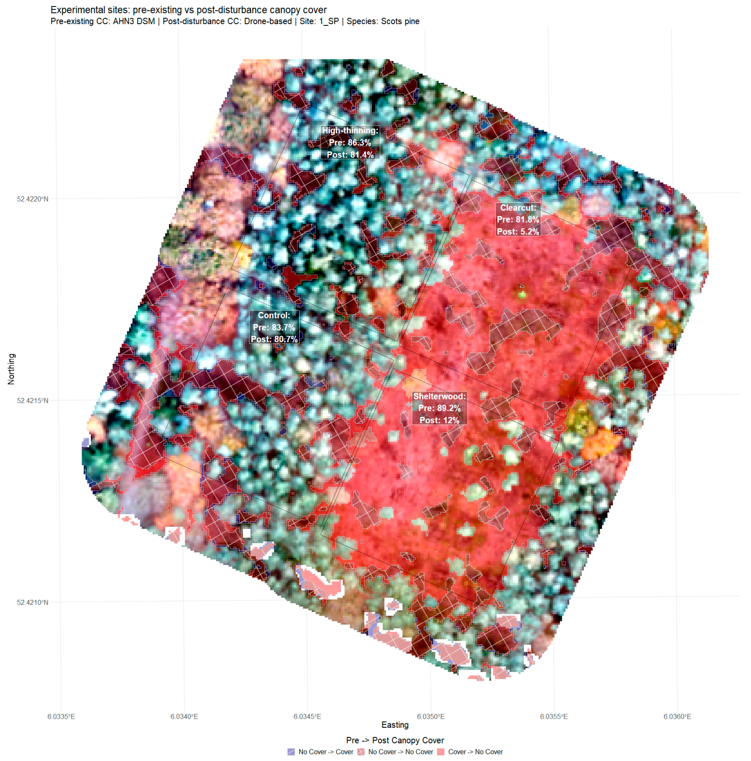
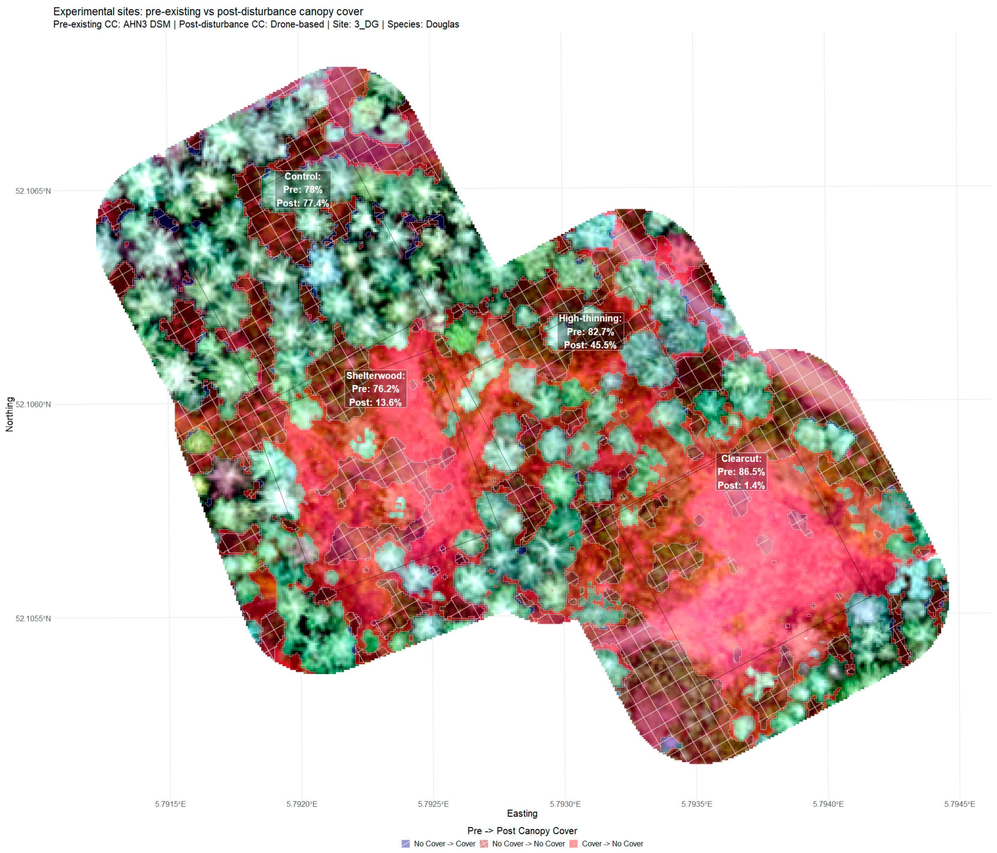
2.1. Study Area and Experimental Sites

The forest study sites are located in the Netherlands, which is characterized by a temperate oceanic climate with an equally distributed yearly average precipitation of 850 mm. Temperatures are mild, with the highest average temperatures occurring in July (18 °C) and the lowest average temperature in February (0.7 °C). Approximately 11% of the total land area of the Netherlands is covered by forest [55]. The forest is highly fragmented on a local and landscape level, managed in some form, and consists of mainly broadleaved deciduous- and coniferous-dominant forest types [55]. The forest in the Netherlands is transitioning from even-aged, monocultural stands toward a higher proportion of mixed forests [55]. Dutch forests are, therefore, relatively diverse in age, composition, management strategies, and spatial configuration.
This study makes use of a forest experiment initiated in 2019, in which fifteen ~1 ha experimental sites were established in even-aged monoculture stands on poor sandy soils within the Netherlands [52,53]. Three dominant tree species are included in the experiment, with each species accounting for five of the fifteen sites: European beech (Fagus sylvatica), Scots pine (Pinus sylvestris), and Douglas fir (Pseudotsuga menziesii). Fourteen of the fifteen sites were used; one of the sites (Beech) could not be used due to insufficient drone imagery quality. The sites vary in stem density, height, biomass distribution, and crown size/shape, depending on the site species, the tree age, and the management history (Table 1). Each site is comprised of four 50 × 50 m sub-sites, in which four different stand density treatments were carried out, which simulate common forest management practices: clearcut, shelterwood, high-thinning, and control. These represent removal of basal area of approximately 100%, 80%, 20%, and 0%, respectively (Figure 1), resulting in a varying pixel-level disturbance severity, even within the same sub-site. The ~0.25 ha sub-sites are not always arranged in a similar fashion but are located as close as possible to one another (Figure 1). The treatments were carried out between 18 February and 15 March 2019, with each treatment implementation lasting between one and three days. During the treatment implementation, the stems were immediately removed from the sites. Further details on the experimental set-up can be found in Vos, de Boer, et al. [52] and Vos, den Ouden, et al. [53].

2.2. Data

2.2.1. Digital Surface Model

In order to estimate the level of canopy cover at high resolution over each site, reference canopy cover maps were necessary for each of the 14 experimental sites for both the pre- and post-treatment periods. The pre-treatment canopy cover map was based on the Digital Surface Model (DSM) product from the third Algemeen Hoogtebestand Nederland (AHN), the Dutch Current Elevation Map. The AHN is a LiDAR-based aerial survey carried out over the Netherlands approximately every five years, with a native resolution of 0.5 m. The data from the third AHN (AHN3) used were acquired between November 2016 and March 2018. The post-treatment map was based on a drone-based photogrammetric nDSM (normalized Digital Surface Model), which had been acquired together with multispectral imagery over the sites in the months following the treatments (May–September 2019) and provided relative heights. This imagery had a native resolution of approximately 0.05 m.

2.2.2. Sentinel-1 Radar

Sentinel-1 A/B Synthetic Aperture Radar (SAR) Ground Range Detected (GRD) data were acquired for the period between January 2016 and April 2022 via the Google Earth Engine (GEE) platform [56]. These data were acquired in Interferometric Wide swath mode in VV and VH polarizations at a resolution of ~20 m (multilook factor of 5 in range direction) with a pixel spacing of 10 m. The incidence angles varied between 31° and 45°. An in-depth description of the pre-processing of the radar data can be found in Appendix A.
For the analyses related to the first objective (Section 3.2 and Section 3.3), the full radar time series was further divided into two sub-time series based on the timing of the treatment implementation in the experimental sites (Figure 2). A pre-treatment time series was defined as all observations between January 2016 and January 2019. No further observations were used in 2019 in order to ensure a roughly equal number of monthly observations across all pre-treatment years and no overlap with the occurrence of the treatments. Similarly, a post-treatment time series was defined as the three-year period between April 2019 and April 2022.

3. Methods

This study focused on assessing the sensitivity of Sentinel-1 backscatter to canopy cover loss severity while taking the effects of radar seasonality, shadow, and layover into account. Figure 2 provides an overview of the pre-processing and analyses performed.

3.1. Preparation of Reference Data

Canopy cover layers were derived from the AHN3 DSM and drone-based nDSM for pre- and post-treatment periods. Shadow and layover coverage were estimated using the post-treatment canopy cover and observation-specific Sentinel-1 incidence and look angles (Figure 2). A full description of the methods used to generate these layers can be found in Appendix A. The Sentinel-1 pixel grid was overlaid with the pre- and post-treatment canopy cover, shadow, and layover layers, providing an estimate of fractional cover for every Sentinel-1 pixel. All parameters derived at a pixel-level can be found in Table 2. Only pixels were selected which were either located entirely within a sub-site or located on the border between two sub-sites. This was done to ensure each pixel represented the tree species of the site in which it was located. In addition, each pixel was assigned a canopy cover class per time period used for further statistical analysis (Table 3). We used classes of canopy cover for two reasons: First, the resampling of each Sentinel-1 image to a common grid introduces a degree of uncertainty in the exact location of each pixel. Each original image could theoretically exhibit an offset of ~5 m from the resampled common grid, introducing minor variations in canopy cover between image acquisitions. Secondly, there was an unbalanced distribution of canopy cover due to the design of the experiment. Pixels with very high (>90%) and very low (<10%) degrees of canopy cover were more prevalent than pixels with partial cover (10–50% and 50–90%). Therefore, it was chosen to use broad classes of canopy cover when performing statistical analysis to determine significant differences between high and low-cover pixels (Table 3).

3.2. Assessing Species-Specific Backscatter Seasonality

The pre-treatment backscatter time series per tree species was analyzed to determine if seasonal C-band Sentinel-1 backscatter patterns differed over closed forests for tree species varying in seasonal phenological patterns. It was hypothesized that monthly backscatter values would differ significantly per species while inter-yearly monthly backscatter values within the same species would not.
Only pixels with a CCPre > 90% in the pre-treatment time series were used (Table 3). The mean backscatter per month was calculated and aggregated over ascending and descending orbits for the entire pre-treatment period. This resulted in 36 mean backscatter values for each pixel. A linear mixed model (LMM) that predicts mean backscatter levels was fit using the lmerTest package (v3.1.3) in R (v4.2.1) [58]. This method is used for longitudinal, non-independent data and allows for their correction by introducing random effects [59,60]. Tree species, month, and year were used as fixed effects, and pixel ID and Site ID as random effects, where pixel ID was implicitly nested within the sites. The local conditions of each site were assumed to introduce random variation which needed to be controlled for, while the pixel ID needed to be identified for repeated measurements. An analysis of variance was then performed, followed by the calculation of relative effect magnitudes of the fixed effects (partial eta squared) using the effectsize package (v0.8.6) [61]. This was done to establish if intra-yearly variation in mean backscatter was significant when considering inter-yearly fluctuations. Multiple comparisons of yearly means between tree species using the Tukey method were performed using the multcomp package (v1.4.17) [62]. Finally, the significance of differences in estimated marginal means between tree species per month was calculated using the emmeans package (v1.6.2.1) [63,64].

3.3. Assessing Backscatter Sensitivity to Canopy Cover

In order to determine the effect of canopy cover on seasonal backscatter, the post-treatment time series was analyzed. This was used instead of the pre-treatment period, as the sites exhibited virtually full coverage before the occurrence of the treatments (Appendix B). It was hypothesized that the radar backscatter would differ throughout the year based on the post-treatment remaining canopy cover (CCPost) and on tree species. Each pixel was considered to have four separate time series observations, keeping both the polarizations and orbits separate since shadow and layover caused by the absence of surrounding canopy cover could be of influence. The backscatter time series of the pixels were filtered to include only the post-treatment time period, aggregated on a monthly basis, and divided into four classes based on CCPost (Table 3). An LMM was fit per species, using the mean backscatter as a dependent variable, month, CCPost class, and orbit as fixed effects, and pixel ID and Site ID as (nested) random effects. Multiple comparisons of means were performed on the CCPost classes, followed by a comparison of estimated marginal means on a monthly basis.

3.4. Assessing Backscatter Sensitivity to Canopy Cover Loss and the Effects of Shadow and Layover

3.4.1. Backscatter Sensitivity to Canopy Cover Loss

The significance of the treatment at a pixel-level (canopy cover loss) was estimated using a causal inference approach, mimicking an operational monitoring set-up under ideal conditions in which the exact date, location, and severity of a disturbance were known. This was done by modeling the temporal trajectory of the backscatter for each pixel, polarization, and orbit direction using the entire time period (2016–2022). In total, this resulted in four polarization- and orbit direction-specific time series per pixel (Table 3).
The causal inference with Bayesian structural time series was carried out using the CausalImpact package (v1.2.7) [65]. The main output of this method is an estimation of the significance of a treatment at a known point in time. This differs from methods focused on detection, in which the probability of occurrence of an event at an unknown point in time is predicted. The treatment significance is obtained by modeling the post-treatment time series for many iterations based on the pre-treatment time series [65]. In addition, a set of correlated synthetic control time series that were unaffected by the treatment can be added to the model [65]. The model then compares the modeled range of probable post-treatment time series with the observed post-treatment time series, producing an estimate of significance. The advantage of causal inference, in which a synthetic control is constructed for each pixel, over simply using the mean of the undisturbed control pixels to estimate treatment significance is that the analysis can be focused on the temporal trajectory of the pixel of interest only. This means the significance can be determined for each pixel separately rather than in relative terms to others, which is the framework used by many operational disturbance monitoring algorithms [17,26]. In turn, the undisturbed control pixels can be used to validate that the model assumptions have been met [65].
Each time series was averaged by month in order to reduce variability introduced by potential Sentinel-1 geolocation errors, resampling artifacts, or environmental influences. Each pixel was assigned a canopy cover loss (ΔCC) class (Table 3). The treatment date per pixel was set to the month following the occurrence of the treatment. Three correlated synthetic control time series per pixel were acquired from the ERA5-Land hourly climate reanalysis dataset, aggregated on a monthly basis, and used as confounding variables: skin reservoir content, daily minimum temperatures, and snow depth (where snow depth > 0.01) [66]. These values were found to be correlated to fluctuations in the radar signal since radar is sensitive to changes in moisture content and temperatures in soil and vegetation [31,40,67,68]. Each value was calculated using only dates corresponding with co-occurring radar observations. The causal inference was applied to each time series separately, using the following parameters: nseasons = 2, season.duration = 6, prior.level.sd = 0.2, alpha = 0.05, and n_it = 1000. The seasonal parameters were chosen based on the expectation that the non-affected backscatter time series would follow a seasonal pattern with distinct summer and winter periods based on the results of the methodology presented in Section 3.2. The prior.level.sd parameter was chosen conservatively so that a maximum of ~10% of pixels with ΔCC of <10% were classified as having exhibited a significant change as a result of the treatment.

3.4.2. Effects of Shadow and Layover

We assessed the effects of shadow and layover on backscatter change magnitude (the difference between pre- and post-treatment mean backscatter values per pixel, Δγ0). It was hypothesized that besides canopy cover loss, shadow, and layover potentially influence mean post-treatment backscatter levels, thereby affecting the significance of a treatment. Weighted linear regressions were performed predicting Δγ0 using different combinations of ΔCC, Srel, and Lrel using observation variances as weights and combined with the causal inference modeling estimates of treatment significance at a pixel level. Four models per species and polarization were fit, with each model employing a different set of independent variables. A base model was fit using only ΔCC as the independent variable. Two models were fit using Srel and Lrel separately, and a full model was fit utilizing both variables and their interaction effects. Adjusted R2 values were derived per model. In addition, adjusted partial R2 values were calculated for Srel and Lrel separately, as well as for both combined [69]. This was done by fitting full and reduced versions of the regression models using the rsq package (v2.5) [70]. The adjusted partial R2 represents the fraction of variance in the full models not explained by the reduced model.

3.5. Monitoring Scenarios

Monitoring scenarios were established in order to explore the potential benefits to detection sensitivity of combining polarization and orbit information over relying on one polarization or orbit direction only. Combining orbit and polarization information is often used in the detection of forest disturbances [26,28]. In addition to increasing the number of available observations, it also allows for the mitigation of the effects of shadow and layover [36,37]. Nine scenarios were established with all combinations of orbit and polarization. No differentiation was made between species since relatively few observations were available at 30–70% ΔCC levels. The 4 baseline scenarios (A1, A2, B1, B2) represent each pixel by single orbit and polarization. The 5 additional combined scenarios (A3, B3, C1, C2, C3) incorporate information from multiple orbits and/or polarizations. In the baseline scenarios, each significant treatment occurrence was thus acknowledged independently. In the combined scenarios, the treatment was regarded as significant if one or more of the input time series was identified as having been significantly affected by the treatment.
The mean fraction of pixels that were identified as affected by the treatment (p < 0.05) was derived per ΔCC class for each scenario. Bootstrap sampling was applied with 1000 iterations per class to obtain 95% confidence intervals. In order to determine which classes experienced significant changes in fractions, pairwise McNemer chi-squared tests were applied per ΔCC class between combined and non-combined scenarios using the rstatix package (v0.7.0) [71].

4. Results

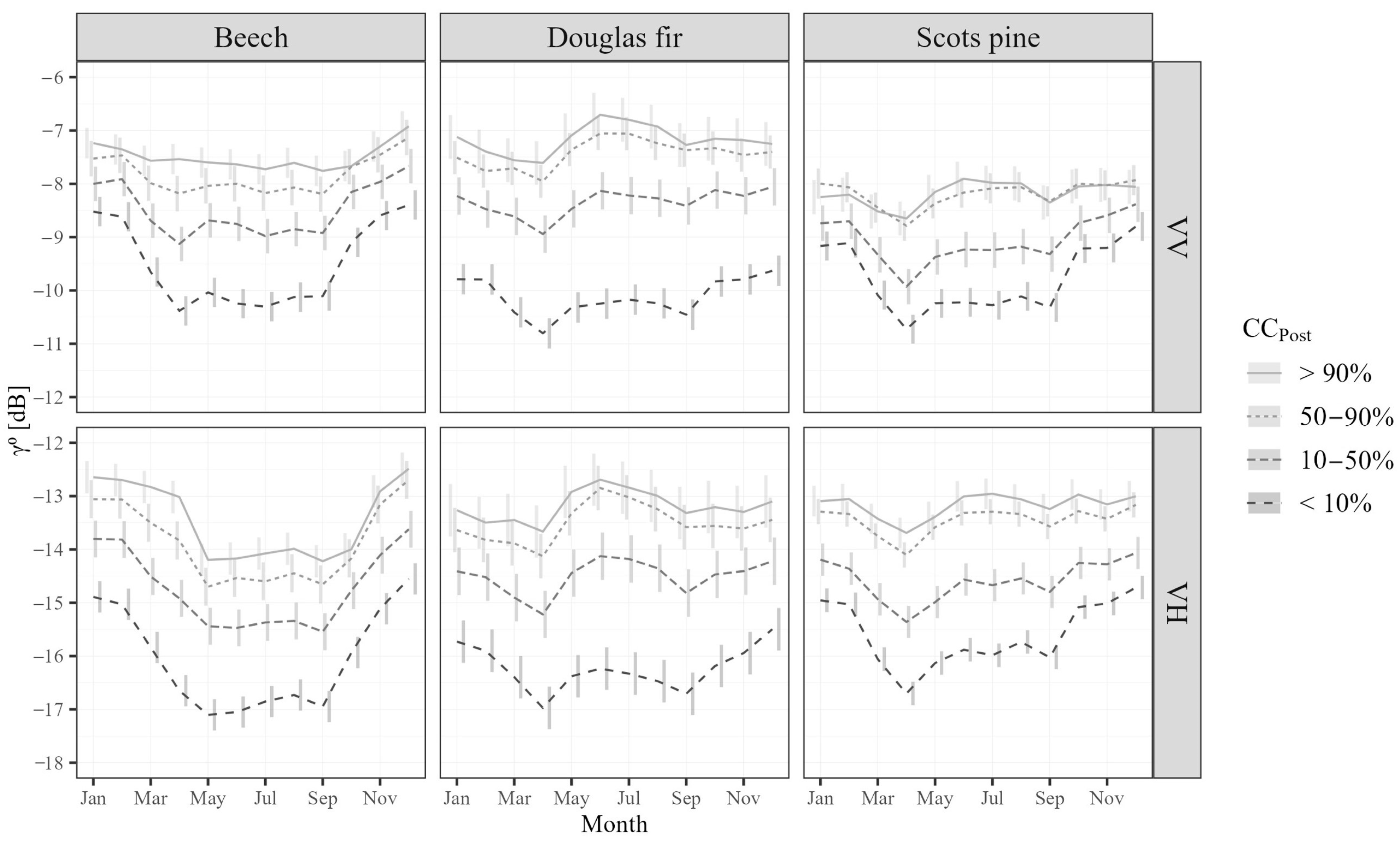
4.1. Backscatter Sensitivity to Species-Specific Seasonality

A seasonal backscatter pattern was visible for each of the three studied tree species. Beech pixels in VH polarization displayed a clear seasonal response, with relatively high values in winter (November–April) compared to the summer months (May–October) (Figure 3). This resulted in a maximum mean difference of ~1.4 dB between the summer and winter months in VH polarization. In VV polarization, the seasonal differences were smaller for Beech, at only ~0.6 dB. In contrast, the Douglas fir and Scots pine exhibited an opposite seasonal response, with higher backscatter values in the summer months and lower values in the winter. These seasonal differences were more pronounced for Douglas fir (VH = ~1.6 dB, VV = ~1.2 dB) than Scots pine (VH = ~0.8 dB, VV = ~0.6 dB), which showed relatively little seasonal variation throughout the year.
There was a significant difference overall between Scots pine and the other species (p < 0.05) in VV and between Douglas fir and Beech in VH polarization (p = 0.02). On a monthly basis, the significance varied, with marginal differences occurring, especially in summer months in both polarizations (Appendix C). The effect sizes of year and its interaction terms were smaller than the effect sizes of other fixed effects and their interaction terms, indicating that species- and month-dependent variations in backscatter were significant despite inter-yearly fluctuations in backscatter (Appendix D).

4.2. Backscatter Sensitivity to Canopy Cover

The mean backscatter of all classes of post-treatment canopy cover (Table 3) differed significantly with the exception of the >90% and 50–90% categories. These differences were marginal for all species and both polarizations. Seasonal patterns in the post-treatment period varied according to the level of canopy cover represented by each pixel (Figure 4). For Beech pixels, lower CCPost was related to an amplification of the seasonal (summer: low, winter: high) backscatter pattern occurring at full canopy cover. The maximum summer–winter difference in mean VH backscatter levels at CCPost > 90% in Beech pixels was ~−1.7 dB, compared to ~−2.5 dB at CCPost < 10%. The seasonal backscatter patterns of Douglas fir and Scots pine (summer: high, winter: low) tended to diminish or even invert at higher CCPost levels. The maximum summer–winter difference in Scots pine in VH at CCPost > 90% was ~ 0.8 dB, compared to ~−2.0 dB at CCPost < 10%. As a result, the seasonal patterns of all species tended toward a ‘summer: low, winter: high’ pattern at lower CCPost levels, regardless of their initial states. The differences between estimated marginal means on a monthly basis could not always be established significantly, especially in winter months for Beech and Scots pine in VV, where differences across the two levels were not significant (Figure 4).

4.3. Backscatter Sensitivity to Canopy Cover Loss and the Effects of Shadow and Layover

The sensitivity to canopy cover loss and the effects of shadow and layover effect are interwoven to a great degree in the case of small-scale, low-intensity disturbances. As such, these factors cannot be assessed on an individual basis. Figure 5 illustrates this interwovenness using an example from a Scots pine site (Appendix B, Figure A9) in which three 10 × 10 m Sentinel-1 pixels are selected. Pixel A did not experience canopy cover loss (ΔCC = 0%, CCPost = 100%), while pixel B (ΔCC = 67.8%, CCPost = 0%) and pixel C (ΔCC = 94%, CCPost = 0%) experienced complete canopy cover loss. The backscatter change magnitude (Δγ0) was low for pixel A, and it was therefore not deemed significantly affected. Pixel B experienced a drop in Δγ0 in both orbits and was significantly affected, as it was likely not influenced by layover and shadow in the middle of the clearing. In contrast, pixel C was located at the edge of the clearing and, therefore, likely affected by layover in the ascending orbit and by shadow in the descending orbit. As a result, it was deemed significantly affected by the treatment (canopy cover loss) in the descending orbit but not in the ascending orbit.
Across all pixels, a negative relationship was found between ΔCC and Δγ0 (Figure 6). The mean Δγ0 at 100% ΔCC was estimated to range from −2.5 dB (±0.3 dB) to −3.1 dB (±0.4 dB) in VH and −1.7 dB (±0.4 dB) to −2.3 dB (±0.4 dB) in VV using the baseline models (without the inclusion of shadow and layover variables). At 50% ΔCC, mean Δγ0 ranged from −1.2 dB (±0.2 dB) to −1.8 dB (±0.2 dB) in VH and −0.7 dB (±0.2 dB) to −1.1 dB (±0.2 dB) in VV. Across both polarizations, Scots pine exhibited the smallest drop in mean Δγ0. Beech and Douglas fir did not significantly differ from one another.
The greatest base model R2 values were found for Scots pine and Beech pixels in VH polarization (Figure 6). In general, a greater proportion of variance was explained in VH than in VV polarization. However, the unexplained variance in both polarizations was relatively high (VV: 66–65%, VH: 62–50%), especially at greater (>75%) ΔCC levels. Fitting full models, including both shadow and layover effects (Srel, Lrel), and their interaction with ΔCC (Figure 6) increased R2 values. It was observed that Srel tended to be related to greater magnitudes of Δγ0, while Lrel tended to be related to smaller magnitudes of Δγ0 (Figure 6). The increased Δγ0 related to high Lrel values resulted in canopy cover loss failing to be recognized as significant by the causal inference methodology.
Adjusted partial R2 values were greater for Lrel than for Srel (Table 4). However, Srel was not found to be significant on its own when added to the base model, while Lrel was only insignificant in the case of Beech. Still, the interaction effects between Srel and Lrel and ΔCC were significant in many cases, while the main effect was not, indicating some explanatory power. Both Srel and Lrel were found to be significant when added in tandem, with the exception of Srel for Douglas fir in VH. The additional explained variance was greater in VV than in VH polarization in all cases except for Lrel Scots pine in VH.

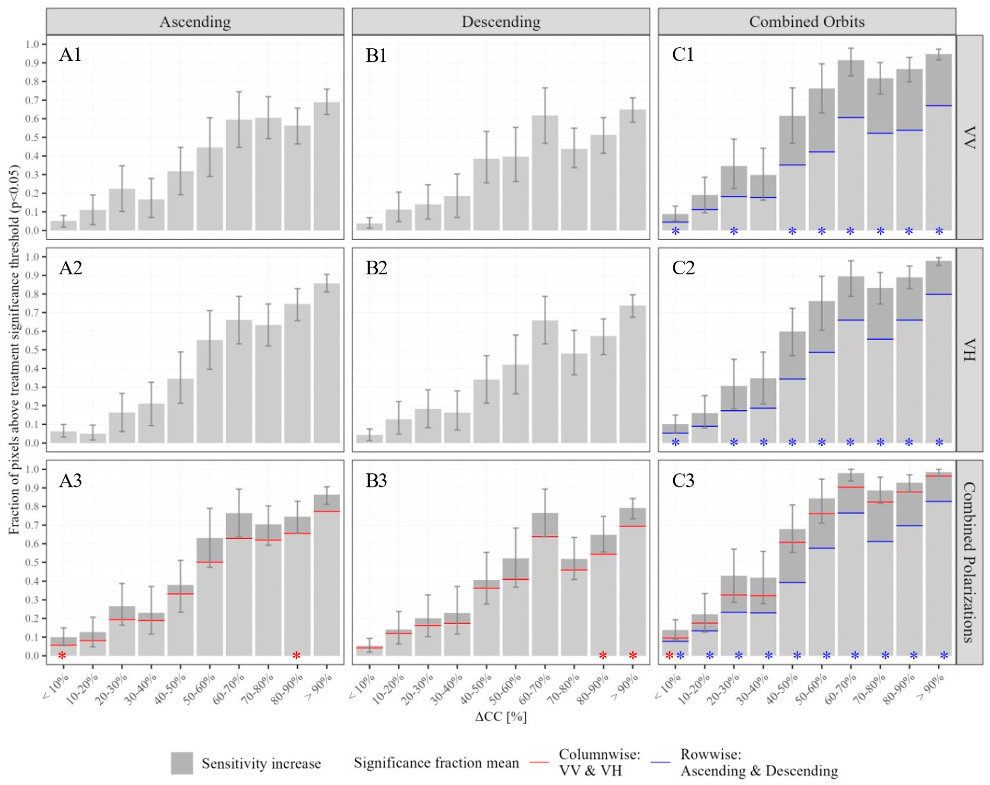
4.4. Monitoring Scenarios

The results for the nine monitoring scenarios (Figure 7) indicated that combining polarization and orbit information at a monitoring level could improve the significance fractions (hereafter referred to as ‘sensitivity’) compared to the sensitivity of each polarization or orbit individually. The combination of polarizations (scenarios A3 and B3) increased the sensitivity by 0.08 (ascending) and 0.07 (descending) on average, corresponding to mean relative increases of ~22% and ~18%. The largest increases of 0.14 (~21%) and 0.13 (~16%) were observed in the 50–60% (ascending) and 60–70% (descending) ΔCC categories, respectively. However, the results of the McNemer chi-square tests showed these increases were mostly insignificant. Combining orbit information further improved the sensitivities, exceeding the increases achieved by combining polarizations. The combination of orbit directions increased the sensitivity in VV (scenario C1) on average by 0.23 (~40%), with the greatest increase observed in the 50–60% ΔCC category (0.34, ~45%). In VH (scenario C2), the average sensitivity was increased by 0.19 (~37%), with the greatest increase in the 50–60% ΔCC category (0.27, ~36%). When both orbit and polarization information were combined (scenario C3), the sensitivity further improved compared to using only combined polarization information. On average, the sensitivities increased by 0.20 (~34%), and a maximum increase of 0.29 (~42%) in the 40–50% ΔCC pixels was found. The largest change in sensitivity from one ΔCC category to the next in the orbit-combined scenarios (C1–3) was found between the 30–40% and the 40–50% ΔCC category, with a sensitivity difference of 0.26.

5. Discussion

5.1. Backscatter Seasonality Is Species-Dependent

The mean backscatter at full canopy cover differed seasonally, with significant differences between species on a monthly basis. Beech exhibited lower backscatter in VH in summer months than in winter months, while Douglas fir and Scots pine exhibited the opposite pattern, with higher values in summer than in winter. These seasonal differences varied between 0.6 and 1.6 dB, depending on species and polarization.
Other studies demonstrated qualitatively similar but quantitatively different results. Broadleaved deciduous forests have been reported to exhibit no seasonal differences in VV and between 0.5 and 2.3 dB in VH, while coniferous forests showed differences between 1.5 and 3.0 in both polarizations [42,72]. Differences in seasonal magnitudes relative to our study might have been related to the relatively short time spans used, as these contained a maximum of 1.5 years of Sentinel-1 observations. A later study using 5 years of Sentinel-1 data [73] reported seasonal differences of 1.8 dB in VH and 0.15 dB in VV for mixed oak and hornbeam stands, similar to our study.
The observed seasonal differences in backscatter have been attributed to various factors. For instance, it has been suggested that the shedding of leaves in the winter of broadleaved deciduous trees reduces the volume scattering component when twigs and branches are masked, leading to lower backscatter [42,45]. In contrast, the higher values of backscatter in summer than winter observed with coniferous trees are suggested to be related to higher leaf area index and higher needle moisture content, while the gradual seasonal removal of moisture from needles to prevent freezing damage, the freezing of understory growth, and snow cover on trees in winter months is related with lower backscatter levels [43,45,46,47,74,75]. Overall, the results demonstrate that the seasonal characteristics of different tree species should be taken into account when developing disturbance detection methods, for instance, by developing pixel- or species-specific stable forest reference periods [26,76,77].

5.2. Canopy Cover Affects Backscatter Mean and Seasonality

The results indicate that canopy cover can affect the yearly mean backscatter, as well as backscatter seasonality, depending on species and its morphological characteristics. All broad classes of canopy cover (Table 3) in the post-treatment period differed significantly from each other, except for high (>90%) and medium-high (50–90%) classes, which demonstrated only marginal differences. This could be due to the co-occurrence of these canopy cover classes with small canopy openings. Since the incidence angles of the short wavelength Sentinel-1 observations over the experimental sites were relatively shallow (31°–45°), the radar signal was likely not able to penetrate to the understory layer through these small openings [28]. In contrast, the significant difference between other canopy cover classes is likely due to the higher contribution of the ground component, which results in lower backscattering than that of the closed canopy. This is in line with a study by Magagi et al. [78] in which C-band backscatter was found to be positively correlated with canopy density and, therefore, to ground and understory backscatter contributions.
The seasonal backscatter patterns at low canopy cover exhibited low backscatter in summer and higher backscatter in winter months, regardless of the tree species. This is likely due to the seasonal differences in moisture levels of the forest floor and understory, which have been shown to have a higher correlation with precipitation than the canopy, resulting in higher ground contributions and higher backscatter levels after precipitation events [79]. An early study with C-band performed in Canada found an opposite seasonal pattern, which could be explained by heavy, persistent snow cover and frost [45,74].
A marginal difference in backscatter was found between canopy cover classes in the winter months in VV polarization compared to VH for Beech and Scots pine, but not for Douglas fir. Relatively high co-polarized backscatter is related to higher canopy penetration, in which of the ground or understory represents a larger contribution to the overall backscatter signal, while VH is related to volume scattering from needles, twigs and branches, which is masked when deciduous foliage is present [46,73,80]. In the case of Douglas fir, the significant differences between canopy cover classes during winter in VV could be related to more needles and branches remaining visible to the sensor when neighboring trees are removed due to its conical canopy shape, with canopy biomass concentrated at a lower stem height compared to the concentration of biomass at the top of the stem of the round Scots pine and Beech canopies [48,81]. This indicates the value of VH over VV for monitoring purposes in (non-frozen) winter conditions, as VH has a more direct relation to canopy cover and is less seasonally dependent across all species studied.
Many management regimes in temperate forests employ silvicultural treatments such as tree harvest, which, depending on the intensity, can result in relatively low canopy densities [13]. Radar backscatter from sparse canopies is, therefore, characterized by highly mixed ground and canopy backscatter contributions [78]. C-band can be useful to detect intensive tree harvest or final felling, but longer wavelengths such as L-band would be advantageous for the characterization of low-intensity management strategies (differentiation between >90% and 50–90% canopy cover classes). L-band has a higher sensitivity to differences in the underlying woody biomass [24] while simultaneously being less influenced by seasonal shifts in foliage.
Methods in time series analysis that attempt to fit seasonal models on a pixel-by-pixel basis have attempted to increase the number of data points with which to fit seasonal models by using spatial context [44,77]. While methods using spatial context are suited for forests in which the seasonality is relatively homogeneous as observed by an (optical) sensor, they are likely not suitable for radar-based detection over mixed-species and sparse canopy cover, such as is the case for temperate forests. Averaging backscatter values from pixels with distinct seasonal patterns as a result of fragmented canopy cover and differing tree species could result in a canceling-out effect. Seasonal patterns of individual pixels would, therefore, be misrepresented, potentially resulting in the confusion of seasonal backscatter behavior with true removal of canopy cover. The pre-disturbance degree of canopy cover is, therefore, an important factor to consider when developing monitoring methodologies.

5.3. Backscatter Sensitivity to Canopy Cover Loss Is Affected by Shadow and Layover

Results suggest that the treatment significance related to canopy cover loss (ΔCC) is affected by radar shadow and layover due to their confounding impact on backscatter change magnitude (Δγ0). A significant Δγ0 at 100% ΔCC, approximately 2–3 dB, was observed across all species. VH polarization was found to be marginally more sensitive to ΔCC than VV, accounting for more variation in pixel-wise mean backscatter magnitude. For partial ΔCC (~50%), Δγ0 approached the absolute radiometric accuracy figure of the Sentinel-1 system, which is 1 dB [82]. Literature on backscatter change magnitude pre- versus post-disturbance is sparse. Olesk et al. reported an average of 2 dB difference for clearcutting and 1.6 dB for thinning across multiple coniferous stands [31]. The mean Δγ0 of our study are similar for Douglas and Scots pine at full and partial canopy cover, but the Δγ0 of individual pixels vary greatly, indicating that pixel-based monitoring requires pixel-scale assessment of canopy cover loss-related Δγ0.
As observed in Section 4.3, Srel tended to be related to greater magnitudes of Δγ0, while Lrel was associated with smaller magnitudes of Δγ0. A high dominance of the layover effect was found to ‘lift’ Δγ0 of observations, causing the canopy cover loss to go unrecognized as significant by the causal inference methodology. There was a large degree of uncertainty in the relationship between both shadow and layover coverage and Δγ0. This could be due to the use of overlapping orbit paths with varying local incidence angles when deriving the shadow and layover layers per pixel. This could especially have an effect on pixels located far away from forest edges, where the coverage varied depending on the orbit path. However, the effects remained significant despite these uncertainties (Table 4).
Adjusted partial R2 values were greater for Lrel than for Srel. This indicates that the shadowing effect might not be as strong as found in previous studies [36], while the layover effect can explain more variance. This could be due to several reasons. First, due to relatively low canopy densities, the radar signal was able to penetrate the canopies of the trees responsible for the shadowing effect, resulting in a non-significant decrease in the signal compared to the removal of the canopy in the pixel of interest. Second, the calculated radar shadow areas were relatively short in length, often not exceeding the resolution of ~20 m, while the layover areas were significantly longer (Figure 5). Backscatter attributed to pixels covered by shadow is, therefore, more likely to be correlated to a higher degree with the nearby forest edge, thereby reducing the explanatory power of shadow [83]. Third, the effect of layover was likely compounded with increased direct scattering, as well as trunk-ground and canopy-ground interactions, which further strengthened the backscatter response [51]. While partial R2 values of Lrel for Scots pine and Beech were relatively equal, they were comparatively low for Douglas fir. The trees in the Douglas fir sites were relatively tall and conically shaped (Table 1). However, the shadow and layover layers assumed the trees were rectangular ‘blocks’. As a result, there is likely a larger degree of overestimation in these layers for Douglas fir, especially at the edges furthest away from the trees responsible for the shadow and layover effects, compared to those in Scots pine and Beech sites. Due to the highly local and small-scale nature of the disturbances and the size of the trees, almost all pixels were affected by shadow or layover in at least one orbit. This implies that if backscatter values from both orbit directions are averaged, the increased backscatter resulting from the layover effect could average out the backscatter drop due to shadowing or canopy removal, leading to the causal inference method failing to identify a true disturbance as significant. The lower canopy density of temperate forests might be a reason why shadow effects might not be as influential as those in the dense, closed canopies of tropical forests. Higher and denser forest canopy would result in a greater degree of attenuation in the case of shadowing [28,35].
Previous studies, such as those by Carstairs et al. and Aquino et al. have made valuable progress in understanding the application of Sentinel-1 radar data for detecting forest disturbances in tropical environments [37,84]. However, their conclusions are not directly applicable to temperate forests. For instance, in Europe, Ruiz-Ramos et al. [77] encountered difficulties in accurately detecting disturbances at the edges of clearcut areas in their study on pixel-based Sentinel-1 detection of forest clearcutting, likely due to shadow and/or layover effects. Overall, the findings of this study underscore the importance of understanding and accounting for these effects when developing methods for the detection of low-intensity disturbances in temperate forests.

5.4. Combining Orbit Directions and Polarizations Increases Detection Sensitivity across Disturbances Severities

The results of the monitoring scenarios highlight the importance of combining both polarizations (VV and VH) and both orbit directions (ascending and descending) when analyzing the loss of canopy cover using Sentinel-1 data. C-band backscatter showed sensitivity to different disturbance severities. However, in the majority of cases, pixels with disturbance severities below 50% were not considered significantly affected by the treatment (Figure 7). A key observation is the increased sensitivity when ascending and descending orbits are combined, as opposed to simply combining VV and VH polarizations (~34% mean relative increase). This outcome implies that the spatial and temporal dynamics of layover and shadow effects play a significant role in determining the overall sensitivity of the Sentinel-1 system to canopy cover loss, confirming results of tropical forest monitoring in which combining polarization and orbit information also improves detection results [26].
It was found that the improvements in sensitivity are not uniform across all canopy cover loss classes. This suggests that certain forest types or conditions might benefit more from the combination of orbit information than others. For instance, pixels with medium- to high- degrees of canopy cover loss exhibited more pronounced improvements in sensitivity when orbits were combined. These pixels were also affected to a greater degree by shadow and layover, as well as additional variance introduced by incidence angles and resulting differences in canopy penetration by the signal [78].
While the benefits of combining polarizations and orbit directions have been demonstrated, further research could investigate the potential synergies and trade-offs between them. Additionally, future studies using L-band radar data should pay special attention to the characterization of shadow and layover effects to aid in the adoption of forthcoming L-band missions such as NISAR, given the uncertainty in applying C-band radar findings to longer wavelengths.

5.5. Limitations

Despite the availability of highly detailed reference data, several limitations are present in the set-up of the experimental plots and the applicability of the findings, as well as in the processing of the radar data. First, the small size and limited number of test sites require careful consideration when applying our findings to research in areas with strongly differing topographical, ecological, and climatic conditions. The sites used in this study were located exclusively on flat terrain and in managed temperate forests dominated by a single species without significant influence of sub-zero temperatures. Understanding the effect of canopy cover change and the influence of seasonality on the signal over forests located on steep terrain, under freezing conditions, and in combination with non-management-related disturbances will require additional experimental research in representative areas. In particular, the occurrence of freezing temperatures and snow cover have been shown to greatly affect C-band backscatter [68,74]. In addition, the effect on the signal of tree species mixtures in forest stands, particularly those including deciduous and evergreen species, could be an important factor to consider, as this complicates the establishment of clear, undisturbed historical periods as is often done in disturbance detection methods [21,76,77]. Shadow and layover effects could also display greater variability in mixed stands than in monospecific stands, as these are dependent on surrounding canopy density and shape, which are more uncertain in the case of mixed stands. Second, inter-observational fluctuations in backscatter on a pixel level due to radar speckle and weather effects were not taken into account but could be of concern in operational monitoring if near-real-time detections are required using individual images [21,67]. Third, the geolocation accuracy and resampling artifacts introduced during the pre-processing of Sentinel imagery add an element of uncertainty to the analysis, as mentioned in Section 3.1. These are especially crucial when performing analyses on small study sites or when developing applications for high-resolution monitoring. However, these uncertainties related to instrument detection capabilities and target size are inherent to the monitoring of subtle changes in the environment. Consequently, additional studies should be done to explore the extent of such uncertainties, for example, when introduced by the fixed pre-processing of data available for cloud-based analysis (e.g., Google Earth Engine). Overall, further highly detailed and site-level experimental studies are required across a range of climatic and topographic gradients examining disturbances from a variety of sources in order to develop accurate disturbance detection methodologies in temperate forests worldwide.

6. Conclusions

The unprecedented detail of the reference data from a network of forest sites with experimentally set disturbance levels allowed us to study the sensitivity of temporally dense C-band radar from Sentinel-1 to management-related temperate forest disturbances. Despite shorter wavelengths and lower canopy-penetrating capabilities than L-band radar, we showed that C-band radar is sensitive to medium- to high-severity pixel-level disturbances. We demonstrated that yearly backscatter patterns are species-specific and that species-specific seasonal patterns depend on per-pixel canopy cover. In addition, it was found that significant differences in post-treatment backscatter levels could be explained not only by canopy cover loss but also by layover and, to a lesser extent, shadow effects. By extension, the implementation of simple monitoring scenarios revealed significant increases in the sensitivity of Sentinel-1 across per-pixel disturbance severities when taking both ascending and descending orbits and VV and VH polarizations into account (~34%). The findings of this study can provide the underpinning for the improvement of operational Sentinel-1-based disturbance monitoring in temperate forests. Combined with dense time series of L-band data from the upcoming NISAR mission and in tandem with optical satellite data, Sentinel-1 C-band radar will prove invaluable to satisfy the increasing requirements imposed by new forest policies for consistent, frequent, and high-resolution forest disturbance monitoring.

Author Contributions

Conceptualization, S.v.d.W., J.R., F.S., G.-J.N. and M.H.; Methodology, S.v.d.W., J.R., F.S. and M.H.; Software, S.v.d.W.; Formal analysis, S.v.d.W.; Investigation, S.v.d.W. and M.V.; Resources, M.V.; Data curation, M.V.; Writing—original draft, S.v.d.W.; Writing—review & editing, J.R., F.S., G.-J.N., M.V. and M.H.; Visualization, S.v.d.W.; Supervision, J.R., F.S., G.-J.N. and M.H.; Funding acquisition, J.R., F.S., G.-J.N. and M.H. All authors have read and agreed to the published version of the manuscript.

Funding

This research was supported by the Open-Earth-Monitor Cyberinfrastructure project (grant agreement No. 101059548), The ForestWard Observatory to Secure Resilience of European Forests (FORWARDS) project (grant agreement No. 101084481), Norway’s Climate and Forest Initiative (NICFI), and the United States Government’s SilvaCarbon program. This research was made possible by the experimental field data provided by Marleen Vos and Frank Sterck, a project funded by the Dutch Research Council (NWO, No. ALWGS.2017.004) and the Dutch Climate Forest Programme funded by the Ministry of Agriculture, Nature Management and Food Quality program led by G.J. Nabuurs, Wageningen Environmental Research. Modified Copernicus Sentinel data [2016–2022] were accessed and pre-processed on the Google Earth Engine platform.

Data Availability Statement

Dataset available on request from the authors.

Acknowledgments

We thank Arjen de Jonge and Eva Meijers for providing writing assistance, and we thank the forest owners, State Forest Service, Kroondomein en Nationaal Park Hoge Veluwe for support with the experimental sites. We would like to thank seven anonymous reviewers for their insightful and constructive feedback, which led to an improved manuscript.

Conflicts of Interest

The authors declare no conflict of interest.

Appendix A

Appendix A.1. Radar Data Pre-Processing

The GRD data in the GEE archive had already undergone orbit file application, border noise removal, thermal noise removal, radiometric calibration, and orthorectification [85]. Additional pre-processing of the GRD data was performed in GEE prior to export following the methodology developed in [86], including additional border noise correction and volumetric radiometric terrain correction using the best available Digital Elevation Model (DEM) in the GEE archive (0.5 m resolution AHN2). No additional speckle filtering was applied in order to reduce spatial averaging effects. No additional corrections for incidence angle backscatter-dependency were carried out, as this effect has been shown to be minor over vegetation [87]. In addition, since monthly-aggregated values of backscatter were used, variation in backscatter due to the use of overlapping orbits over individual pixels was smoothed out. The data in both orbit directions were resampled to a common grid with 10 m pixel spacing using the nearest neighbor method and exported for further analysis in R (v4.2.1).
It is well known that C-band radar can be affected by freezing temperatures and snow cover [31,40,67,68]. Using climate data from the ERA5-Land dataset [66], it was found that over all the sites, on average, only ~5 observations per year were obtained where the daily temperature was below −5 °C, and only ~3 observations where snow cover was greater than 5 cm. Assuming minimal influence of these factors in the experimental sites, no extra corrections were carried out.

Appendix A.2. Canopy Cover Layer Generation

The drone-based nDSM (post-treatment) was aggregated, resampled, and reprojected to the same resolution and projection as the AHN3 DSM (pre-treatment). Then, the drone-based nDSM was co-registered with the AHN3 DSM to limit any spatial offset between the datasets.
Since these were not directly comparable, it was chosen to develop a binary mask representing canopy and non-canopy areas from each DSM using an adaptive filter [88]. The filter used a 151 × 151-pixel window size. It was assumed that a pixel representing the forest floor would occur somewhere within the window, which could be represented by the minimum value, and that there was a degree of non-canopy understory vegetation represented by the standard deviation. The canopy cover was assigned to the central pixel if it exceeded a threshold calculated as the minimum value, plus 0.75 times the standard deviation of values within the window.
In order to determine where the canopy cover was removed, the difference between the pre- and post-treatment canopy cover maps was determined. Maps of all sites can be found in Appendix B, in which also the pre- and post- treatment canopy cover are represented.

Appendix A.3. Shadow and Layover Layers Generation

Shadow and layover layers were derived spatially for the post-treatment period. Note that while this study refers to these geometric distortions as shadow and layover, these are partial effects, in which the signal is only partially diminished or amplified as a result of interaction with the canopy [28,51,89].
Approximate shadow and layover layers could be derived for each orbit direction and relative orbit path. These were calculated by converting the canopy cover mask for each site to vector format and assigning the corresponding site-specific mean tree height to each vector. The shadow package (v0.7.1) [90] was employed to simulate the theoretical spatial distribution of shadow and layover using the mean tree height, satellite azimuth angle, and look angle as inputs. The layover and shadow layers were calculated as a raster for each observation at 0.5 m resolution, after which the modal value, representing the most occurring shadow/layover coverage (or absence), was assigned to each 0.5 m pixel. In addition, the shadow- and layover layers were masked by the canopy cover layer to avoid overlapping shadow- and layover with the canopy cover itself.
It was assumed that within-site tree height variation and the 3D crown shape at the tree level would not significantly impact the outcomes. This is because all sites were even-aged, resulting in minor within-site tree height fluctuation and because differences in incidence angles between acquisitions smooth out shadow and layover spatially when averaged over time.

Appendix B

Figure A1. Pre-versus post-treatment canopy cover. Species: Beech. Site ID: 1_BE.
Remotesensing 16 01553 g0a1
Figure A2. Pre-versus post-treatment canopy cover. Species: Douglas Fir. Site ID: 1_DG.
Remotesensing 16 01553 g0a2
Figure A3. Pre- versus post-treatment canopy cover. Species: Scots Pine. Site ID: 1_SP.
Remotesensing 16 01553 g0a3
Figure A4. Pre- versus post-treatment canopy cover. Species: Beech. Site ID: 2_BE.
Remotesensing 16 01553 g0a4
Figure A5. Pre- versus post-treatment canopy cover. Species: Douglas Fir. Site ID: 2_DG.
Remotesensing 16 01553 g0a5
Figure A6. Pre- versus post-treatment canopy cover. Species: Scots Pine. Site ID: 2_SP.
Remotesensing 16 01553 g0a6
Figure A7. Pre- versus post-treatment canopy cover. Species: Beech. Site ID: 3_BE.
Remotesensing 16 01553 g0a7
Figure A8. Pre- versus post-treatment canopy cover. Species: Douglas Fir. Site ID: 3_DG.
Remotesensing 16 01553 g0a8
Figure A9. Pre- versus post-treatment canopy cover. Species: Scots Pine. Site ID: 3_SP.
Remotesensing 16 01553 g0a9
Figure A10. Pre- versus post-treatment canopy cover. Species: Douglas Fir. Site ID: 4_DG.
Remotesensing 16 01553 g0a10
Figure A11. Pre- versus post-treatment canopy cover. Species: Scots Pine. Site ID: 4_SP.
Remotesensing 16 01553 g0a11
Figure A12. Pre- versus post-treatment canopy cover. Species: Beech. Site ID: 5_BE.
Remotesensing 16 01553 g0a12
Figure A13. Pre- versus post-treatment canopy cover. Species: Douglas Fir. Site ID: 5_DG.
Remotesensing 16 01553 g0a13
Figure A14. Pre- versus post-treatment canopy cover. Species: Scots Pine. Site ID: 5_SP.
Remotesensing 16 01553 g0a14

Appendix C

Table A1. Pairwise marginal means contrast significance for VH polarization.
Contrast–VH Polarization
Beech—DouglasBeech—Scots PineDouglas—Scots Pine
Month1<0.001<0.001<0.001
2<0.001<0.0010.010
3<0.001<0.0010.026
4<0.001<0.0010.286
50.1300.2930.886
6<0.0010.0370.269
70.0170.3240.345
80.1520.0800.951
90.8330.7830.995
100.9990.2880.267
11<0.0010.0030.054
12<0.001<0.0010.002
Table A2. Pairwise marginal means contrast significance for VV polarization.
Contrast–VV Polarization
Beech—DouglasBeech—Scots PineDouglas—Scots Pine
Month1<0.001<0.0010.006
2<0.001<0.001<0.001
30.002<0.001<0.001
40.095<0.001<0.001
50.945<0.001<0.001
60.831<0.001<0.001
70.193<0.001<0.001
80.852<0.001<0.001
90.995<0.001<0.001
100.936<0.001<0.001
110.011<0.0010.003
120.003<0.0010.001

Appendix D

Table A3. Effect size of fixed effects expressed as partial eta squared.
VV PolarizationVH Polarization
Partial eta SquaredConfidence Interval Partial eta SquaredConfidence Interval
Fixed Effectsspecies0.81(0.49, 0.91)0.43(0.00, 0.70)
year0.00(0.00, 0.00)0.01(0.00, 0.01)
month0.10(0.09, 0.11)0.10(0.09, 0.10)
species:year0.00(0.00, 0.01)0.00(0.00, 0,00)
species:month0.05(0.05, 0.06)0.28(0.27, 0.29)
year:month0.10(0.09, 0.11)0.14(0.13, 0.15)
species:year:month0.02(0.01, 0.02) 0.02(0.02, 0.02)

References

  1. Nabuurs, G.-J.; Hatab, A.A.; Bustamante, M.; Clark, H.; Havlík, P.; Ninan, K.N.; Popp, A.; Roe, S.; Aoki, L.; Angers, D.; et al. 2022: Agriculture, Forestry and Other Land Uses (AFOLU). In IPCC, 2022: Climate Change 2022: Mitigation of Climate Change. Contribution of Working Group III to the Sixth Assessment Report of the Intergovernmental Panel on Climate Change; Cambridge University Press: Cambridge, UK; New York, NY, USA, 2022; ISBN 978-1-00-915792-6. [Google Scholar]
  2. European Commission. New EU Forest Strategy for 2030; European Commission: Brussels, Belgium, 2021. [Google Scholar]
  3. Canadian Council of Forest Ministers. Renewed Forest Bioeconomy Framework. 2021. Available online: https://www.ccfm.org/releases/renewed-forest-bioeconomy-framework/ (accessed on 15 February 2023).
  4. Bastos, A.; Ciais, P.; Friedlingstein, P.; Sitch, S.; Pongratz, J.; Fan, L.; Wigneron, J.P.; Weber, U.; Reichstein, M.; Fu, Z.; et al. Direct and Seasonal Legacy Effects of the 2018 Heat Wave and Drought on European Ecosystem Productivity. Sci. Adv. 2020, 6, eaba2724. [Google Scholar] [CrossRef] [PubMed]
  5. Cohen, W.B.; Yang, Z.; Stehman, S.V.; Schroeder, T.A.; Bell, D.M.; Masek, J.G.; Huang, C.; Meigs, G.W. Forest Disturbance across the Conterminous United States from 1985–2012: The Emerging Dominance of Forest Decline. For. Ecol. Manag. 2016, 360, 242–252. [Google Scholar] [CrossRef]
  6. McDowell, N.G.; Allen, C.D.; Anderson-Teixeira, K.; Aukema, B.H.; Bond-Lamberty, B.; Chini, L.; Clark, J.S.; Dietze, M.; Grossiord, C.; Hanbury-Brown, A.; et al. Pervasive Shifts in Forest Dynamics in a Changing World. Science 2020, 368, eaaz9463. [Google Scholar] [CrossRef]
  7. Patacca, M.; Lindner, M.; Lucas-Borja, M.E.; Cordonnier, T.; Fidej, G.; Gardiner, B.; Hauf, Y.; Jasinevičius, G.; Labonne, S.; Linkevičius, E.; et al. Significant Increase in Natural Disturbance Impacts on European Forests since 1950. Glob. Chang. Biol. 2023, 29, 1359–1376. [Google Scholar] [CrossRef] [PubMed]
  8. Seidl, R.; Thom, D.; Kautz, M.; Martin-Benito, D.; Peltoniemi, M.; Vacchiano, G.; Wild, J.; Ascoli, D.; Petr, M.; Honkaniemi, J.; et al. Forest Disturbances under Climate Change. Nat. Clim. Chang. 2017, 7, 395–402. [Google Scholar] [CrossRef] [PubMed]
  9. Ceccherini, G.; Duveiller, G.; Grassi, G.; Lemoine, G.; Avitabile, V.; Pilli, R.; Cescatti, A. Abrupt Increase in Harvested Forest Area over Europe after 2015. Nature 2020, 583, 72–77. [Google Scholar] [CrossRef] [PubMed]
  10. Palahí, M.; Valbuena, R.; Senf, C.; Acil, N.; Pugh, T.A.M.; Sadler, J.; Seidl, R.; Potapov, P.; Gardiner, B.; Hetemäki, L.; et al. Concerns about Reported Harvests in European Forests. Nature 2021, 592, E15–E17. [Google Scholar] [CrossRef] [PubMed]
  11. Sebald, J.; Senf, C.; Seidl, R. Human or Natural? Landscape Context Improves the Attribution of Forest Disturbances Mapped from Landsat in Central Europe. Remote Sens. Environ. 2021, 262, 112502. [Google Scholar] [CrossRef]
  12. Hirschmugl, M.; Gallaun, H.; Dees, M.; Datta, P.; Deutscher, J.; Koutsias, N.; Schardt, M. Methods for Mapping Forest Disturbance and Degradation from Optical Earth Observation Data: A Review. Curr. For. Rep. 2017, 3, 32–45. [Google Scholar] [CrossRef]
  13. Senf, C.; Seidl, R. Mapping the Forest Disturbance Regimes of Europe. Nat. Sustain. 2021, 4, 63–70. [Google Scholar] [CrossRef]
  14. Francini, S.; McRoberts, R.E.; D’Amico, G.; Coops, N.C.; Hermosilla, T.; White, J.C.; Wulder, M.A.; Marchetti, M.; Mugnozza, G.S.; Chirici, G. An Open Science and Open Data Approach for the Statistically Robust Estimation of Forest Disturbance Areas. Int. J. Appl. Earth Obs. Geoinf. 2022, 106, 102663. [Google Scholar] [CrossRef]
  15. Giannetti, F.; Pecchi, M.; Travaglini, D.; Francini, S.; D’Amico, G.; Vangi, E.; Cocozza, C.; Chirici, G. Estimating VAIA Windstorm Damaged Forest Area in Italy Using Time Series Sentinel-2 Imagery and Continuous Change Detection Algorithms. Forests 2021, 12, 680. [Google Scholar] [CrossRef]
  16. Lastovicka, J.; Svec, P.; Paluba, D.; Kobliuk, N.; Svoboda, J.; Hladky, R.; Stych, P. Sentinel-2 Data in an Evaluation of the Impact of the Disturbances on Forest Vegetation. Remote Sens. 2020, 12, 1914. [Google Scholar] [CrossRef]
  17. Senf, C.; Pflugmacher, D.; Hostert, P.; Seidl, R. Using Landsat Time Series for Characterizing Forest Disturbance Dynamics in the Coupled Human and Natural Systems of Central Europe. ISPRS J. Photogramm. Remote Sens. 2017, 130, 453–463. [Google Scholar] [CrossRef] [PubMed]
  18. Thonfeld, F.; Gessner, U.; Holzwarth, S.; Kriese, J.; da Ponte, E.; Huth, J.; Kuenzer, C. A First Assessment of Canopy Cover Loss in Germany’s Forests after the 2018–2020 Drought Years. Remote Sens. 2022, 14, 562. [Google Scholar] [CrossRef]
  19. Gao, Y.; Skutsch, M.; Paneque-Gálvez, J.; Ghilardi, A. Remote Sensing of Forest Degradation: A Review. Environ. Res. Lett. 2020, 15, 103001. [Google Scholar] [CrossRef]
  20. Pantze, A.; Santoro, M.; Fransson, J.E.S. Change Detection of Boreal Forest Using Bi-Temporal ALOS PALSAR Backscatter Data. Remote Sens. Environ. 2014, 155, 120–128. [Google Scholar] [CrossRef]
  21. Reiche, J.; Hamunyela, E.; Verbesselt, J.; Hoekman, D.; Herold, M. Improving Near-Real Time Deforestation Monitoring in Tropical Dry Forests by Combining Dense Sentinel-1 Time Series with Landsat and ALOS-2 PALSAR-2. Remote Sens. Environ. 2018, 204, 147–161. [Google Scholar] [CrossRef]
  22. Shimada, M.; Itoh, T.; Motooka, T.; Watanabe, M.; Shiraishi, T.; Thapa, R.; Lucas, R. New Global Forest/Non-Forest Maps from ALOS PALSAR Data (2007–2010). Remote Sens. Environ. 2014, 155, 13–31. [Google Scholar] [CrossRef]
  23. Watanabe, M.; Koyama, C.N.; Hayashi, M.; Nagatani, I.; Tadono, T.; Shimada, M. Refined Algorithm for Forest Early Warning System with ALOS-2/PALSAR-2 ScanSAR Data in Tropical Forest Regions. Remote Sens. Environ. 2021, 265, 112643. [Google Scholar] [CrossRef]
  24. Tanase, M.A.; Villard, L.; Pitar, D.; Apostol, B.; Petrila, M.; Chivulescu, S.; Leca, S.; Borlaf-Mena, I.; Pascu, I.S.; Dobre, A.C.; et al. Synthetic Aperture Radar Sensitivity to Forest Changes: A Simulations-Based Study for the Romanian Forests. Sci. Total Environ. 2019, 689, 1104–1114. [Google Scholar] [CrossRef] [PubMed]
  25. Hethcoat, M.G.; Carreiras, J.M.B.; Edwards, D.P.; Bryant, R.G.; Quegan, S. Detecting Tropical Selective Logging with C-Band SAR Data May Require a Time Series Approach. Remote Sens. Environ. 2021, 259, 112411. [Google Scholar] [CrossRef]
  26. Reiche, J.; Mullissa, A.; Slagter, B.; Gou, Y.; Tsendbazar, N.E.; Odongo-Braun, C.; Vollrath, A.; Weisse, M.J.; Stolle, F.; Pickens, A.; et al. Forest Disturbance Alerts for the Congo Basin Using Sentinel-1. Environ. Res. Lett. 2021, 16, 024005. [Google Scholar] [CrossRef]
  27. Doblas Prieto, J.; Lima, L.; Mermoz, S.; Bouvet, A.; Reiche, J.; Watanabe, M.; Sant Anna, S.; Shimabukuro, Y. Inter-Comparison of Optical and SAR-Based Forest Disturbance Warning Systems in the Amazon Shows the Potential of Combined SAR-Optical Monitoring. Int. J. Remote Sens. 2023, 44, 59–77. [Google Scholar] [CrossRef]
  28. Hoekman, D.; Kooij, B.; Quiñones, M.; Vellekoop, S.; Carolita, I.; Budhiman, S.; Arief, R.; Roswintiarti, O. Wide-Area Near-Real-Time Monitoring of Tropical Forest Degradation and Deforestation Using Sentinel-1. Remote Sens. 2020, 12, 3263. [Google Scholar] [CrossRef]
  29. Rüetschi, M.; Small, D.; Waser, L.T. Rapid Detection of Windthrows Using Sentinel-1 C-Band SAR Data. Remote Sens. 2019, 11, 115. [Google Scholar] [CrossRef]
  30. Dascălu, A.; Catalão, J.; Navarro, A. Detecting Deforestation Using Logistic Analysis and Sentinel-1 Multitemporal Backscatter Data. Remote Sens. 2023, 15, 290. [Google Scholar] [CrossRef]
  31. Olesk, A.; Voormansik, K.; Pohjala, M.; Noorma, M. Forest Change Detection from Sentinel-1 and ALOS-2 Satellite Images. In Proceedings of the 2015 IEEE 5th Asia-Pacific Conference on Synthetic Aperture Radar (APSAR), Singapore, 1–4 September 2015; IEEE: Singapore, 2015; pp. 522–527. [Google Scholar]
  32. Belenguer-Plomer, M.A.; Tanase, M.A.; Fernandez-Carrillo, A.; Chuvieco, E. Burned Area Detection and Mapping Using Sentinel-1 Backscatter Coefficient and Thermal Anomalies. Remote Sens. Environ. 2019, 233, 111345. [Google Scholar] [CrossRef]
  33. De Luca, G.; Silva, J.M.N.; Modica, G. A Workflow Based on Sentinel-1 SAR Data and Open-Source Algorithms for Unsupervised Burned Area Detection in Mediterranean Ecosystems. GISci. Remote Sens. 2021, 58, 516–541. [Google Scholar] [CrossRef]
  34. JRC. Forest Landscape in Europe: Pattern, Fragmentation and Connectivity; Publications Office: Luxembourg, 2013. [Google Scholar]
  35. Ballère, M.; Bouvet, A.; Mermoz, S.; Le Toan, T.; Koleck, T.; Bedeau, C.; André, M.; Forestier, E.; Frison, P.-L.; Lardeux, C. SAR Data for Tropical Forest Disturbance Alerts in French Guiana: Benefit over Optical Imagery. Remote Sens. Environ. 2021, 252, 112159. [Google Scholar] [CrossRef]
  36. Bouvet, A.; Mermoz, S.; Ballère, M.; Koleck, T.; Le Toan, T. Use of the SAR Shadowing Effect for Deforestation Detection with Sentinel-1 Time Series. Remote Sens. 2018, 10, 1250. [Google Scholar] [CrossRef]
  37. Carstairs, H.; Mitchard, E.T.A.; McNicol, I.; Aquino, C.; Chezeaux, E.; Ebanega, M.O.; Dikongo, A.M.; Disney, M. Sentinel-1 Shadows Used to Quantify Canopy Loss from Selective Logging in Gabon. Remote Sens. 2022, 14, 4233. [Google Scholar] [CrossRef]
  38. Fox, T.R.; Jokela, E.J.; Allen, H.L. The Development of Pine Plantation Silviculture in the Southern United States. J. For. 2007, 105, 337–347. [Google Scholar] [CrossRef]
  39. Gilliam, F.S. Forest Ecosystems of Temperate Climatic Regions: From Ancient Use to Climate Change. New Phytol. 2016, 212, 871–887. [Google Scholar] [CrossRef] [PubMed]
  40. Kaiser, P.; Buddenbaum, H.; Nink, S.; Hill, J. Potential of Sentinel-1 Data for Spatially and Temporally High-Resolution Detection of Drought Affected Forest Stands. Forests 2022, 13, 2148. [Google Scholar] [CrossRef]
  41. Pulliainen, J.; Hari, P.; Hallikainen, M.; Patrikainen, N.; Peramaki, M.; Kolari, P. Monitoring of Soil Moisture and Vegetation Water Content Variations in Boreal Forest from C-Band SAR Data. In Proceedings of the IEEE International Geoscience and Remote Sensing Symposium, IGARSS ’04, Anchorage, AK, USA, 20–24 September 2004; IEEE: Anchorage, AK, USA, 2004; Volume 2, pp. 1013–1016. [Google Scholar]
  42. Dostálová, A.; Wagner, W.; Milenković, M.; Hollaus, M. Annual Seasonality in Sentinel-1 Signal for Forest Mapping and Forest Type Classification. Int. J. Remote Sens. 2018, 39, 7738–7760. [Google Scholar] [CrossRef]
  43. Dostálová, A.; Lang, M.; Ivanovs, J.; Waser, L.T.; Wagner, W. European Wide Forest Classification Based on Sentinel-1 Data. Remote Sens. 2021, 13, 337. [Google Scholar] [CrossRef]
  44. Hamunyela, E.; Verbesselt, J.; Herold, M. Using Spatial Context to Improve Early Detection of Deforestation from Landsat Time Series. Remote Sens. Environ. 2016, 172, 126–138. [Google Scholar] [CrossRef]
  45. Ahern, F.J.; Leckie, D.J.; Drieman, J.A. Seasonal Changes in Relative C-Band Backscatter of Northern Forest Cover Types. IEEE Trans. Geosci. Remote Sens. 1993, 31, 668–680. [Google Scholar] [CrossRef]
  46. Rüetschi, M.; Schaepman, M.; Small, D. Using Multitemporal Sentinel-1 C-Band Backscatter to Monitor Phenology and Classify Deciduous and Coniferous Forests in Northern Switzerland. Remote Sens. 2017, 10, 55. [Google Scholar] [CrossRef]
  47. Udali, A.; Lingua, E.; Persson, H.J. Assessing Forest Type and Tree Species Classification Using Sentinel-1 C-Band SAR Data in Southern Sweden. Remote Sens. 2021, 13, 3237. [Google Scholar] [CrossRef]
  48. Borlaf-Mena, I.; García-Duro, J.; Santoro, M.; Villard, L.; Badea, O.; Tanase, M.A. Seasonality and Directionality Effects on Radar Backscatter Are Key to Identify Mountain Forest Types with Sentinel-1 Data. Remote Sens. Environ. 2023, 296, 113728. [Google Scholar] [CrossRef]
  49. Dubois, C.; Mueller, M.M.; Pathe, C.; Jagdhuber, T.; Cremer, F.; Thiel, C.; Schmullius, C. Characterization of land cover seasonality in sentinel-1 time series data. ISPRS Ann. Photogramm. Remote Sens. Spat. Inf. Sci. 2020; V-3-2020, 97–104. [Google Scholar] [CrossRef]
  50. Woodhouse, I.H. Introduction to Microwave Remote Sensing; Taylor&Francis: Boca Raton, FL, USA, 2006; ISBN 978-0-415-27123-3. [Google Scholar]
  51. Sun, G.; Ranson, K.J. A Three-Dimensional Radar Backscatter Model of Forest Canopies. IEEE Trans. Geosci. Remote Sens. 1995, 33, 372–382. [Google Scholar] [CrossRef]
  52. Vos, M.A.E.; de Boer, D.; de Vries, W.; den Ouden, J.; Sterck, F.J. Aboveground Carbon and Nutrient Distributions Are Hardly Associated with Canopy Position for Trees in Temperate Forests on Poor and Acidified Sandy Soils. For. Ecol. Manag. 2023, 529, 120731. [Google Scholar] [CrossRef]
  53. Vos, M.A.E.; den Ouden, J.; Hoosbeek, M.; Valtera, M.; de Vries, W.; Sterck, F. The Sustainability of Timber and Biomass Harvest in Perspective of Forest Nutrient Uptake and Nutrient Stocks. For. Ecol. Manag. 2023, 530, 120791. [Google Scholar] [CrossRef]
  54. Iwasaki, A.; Noda, T. A Framework for Quantifying the Relationship between Intensity and Severity of Impact of Disturbance across Types of Events and Species. Sci. Rep. 2018, 8, 795. [Google Scholar] [CrossRef]
  55. Schelhaas, M.-J.; Clerkx, S.; Lerink, B. Zevende Nederlandse Bosinventarisatie: 2017–2021; Wettelijke Onderzoekstaken Natuur & Milieu: Wageningen, The Netherlands, 2022. [Google Scholar]
  56. Gorelick, N.; Hancher, M.; Dixon, M.; Ilyushchenko, S.; Thau, D.; Moore, R. Google Earth Engine: Planetary-Scale Geospatial Analysis for Everyone. Remote Sens. Environ. 2017, 202, 18–27. [Google Scholar] [CrossRef]
  57. Fletcher, K. (Ed.) Sentinel-1: ESA’s Radar Observatory Mission for GMES Operational Services; ESA SP-1322/1; ESA Communications: Noordwijk, The Netherlands, 2012; ISBN 978-92-9221-418-0. [Google Scholar]
  58. Kuznetsova, A.; Brockhoff, P.B.; Christensen, R.H.B. LmerTest Package: Tests in Linear Mixed Effects Models. J. Stat. Soft. 2017, 82, 26. [Google Scholar] [CrossRef]
  59. Cnaan, A.; Laird, N.M.; Slasor, P. Using the General Linear Mixed Model to Analyse Unbalanced Repeated Measures and Longitudinal Data. Statist. Med. 1997, 16, 2349–2380. [Google Scholar] [CrossRef]
  60. Millard, K.; Thompson, D.; Parisien, M.-A.; Richardson, M. Soil Moisture Monitoring in a Temperate Peatland Using Multi-Sensor Remote Sensing and Linear Mixed Effects. Remote Sens. 2018, 10, 903. [Google Scholar] [CrossRef]
  61. Ben-Shachar, M.; Lüdecke, D.; Makowski, D. Effectsize: Estimation of Effect Size Indices and Standardized Parameters. JOSS 2020, 5, 2815. [Google Scholar] [CrossRef]
  62. Hothorn, T.; Bretz, F.; Westfall, P. Simultaneous Inference in General Parametric Models. Biom. J. 2008, 50, 346–363. [Google Scholar] [CrossRef]
  63. Lenth, R. emmeans: Estimated Marginal Means, aka Least-Squares Means. Available online: https://CRAN.R-project.org/package=emmeans (accessed on 15 February 2023).
  64. Searle, S.R.; Speed, F.M.; Milliken, G.A. Population Marginal Means in the Linear Model: An Alternative to Least Squares Means. Am. Stat. 1980, 34, 216–221. [Google Scholar] [CrossRef]
  65. Brodersen, K.H.; Gallusser, F.; Koehler, J.; Remy, N.; Scott, S.L. Inferring Causal Impact Using Bayesian Structural Time-Series Models. Ann. Appl. Stat. 2015, 9, 247–274. [Google Scholar] [CrossRef]
  66. Muñoz-Sabater, J.; Dutra, E.; Agustí-Panareda, A.; Albergel, C.; Arduini, G.; Balsamo, G.; Boussetta, S.; Choulga, M.; Harrigan, S.; Hersbach, H.; et al. ERA5-Land: A State-of-the-Art Global Reanalysis Dataset for Land Applications. Earth Syst. Sci. Data 2021, 13, 4349–4383. [Google Scholar] [CrossRef]
  67. Benninga, H.-J.; van der Velde, R.; Su, Z. Impacts of Radiometric Uncertainty and Weather-Related Surface Conditions on Soil Moisture Retrievals with Sentinel-1. Remote Sens. 2019, 11, 2025. [Google Scholar] [CrossRef]
  68. Cohen, J.; Rautiainen, K.; Lemmetyinen, J.; Smolander, T.; Vehviläinen, J.; Pulliainen, J. Sentinel-1 Based Soil Freeze/Thaw Estimation in Boreal Forest Environments. Remote Sens. Environ. 2021, 254, 112267. [Google Scholar] [CrossRef]
  69. Zhang, D. A Coefficient of Determination for Generalized Linear Models. Am. Stat. 2017, 71, 310–316. [Google Scholar] [CrossRef]
  70. Zhang, D. Package ‘Rsq’ 2022. Available online: https://cran.r-project.org/web/packages/rsq/rsq.pdf (accessed on 15 February 2023).
  71. Kassambara, A. Practical Statistics in R II—Comparing Groups: Numerical Variables, 1st ed.; Datanovia: Montpellier, France, 2019. [Google Scholar]
  72. Dostálová, A.; Milenković, M.; Hollaus, M.; Wagner, W. Influence of Forest Structure on the Sentinel-1 Backscatter Variation—Analysis with Full-Waveform LIDAR Data. In Proceedings of the Living Planet Symposium, Prague, Czech Republic, 9–13 May 2016; Volume 740, p. 202. [Google Scholar]
  73. Soudani, K.; Delpierre, N.; Berveiller, D.; Hmimina, G.; Vincent, G.; Morfin, A.; Dufrêne, É. Potential of C-Band Synthetic Aperture Radar Sentinel-1 Time-Series for the Monitoring of Phenological Cycles in a Deciduous Forest. Int. J. Appl. Earth Obs. Geoinf. 2021, 104, 102505. [Google Scholar] [CrossRef]
  74. Lemmetyinen, J.; Ruiz, J.J.; Cohen, J.; Haapamaa, J.; Kontu, A.; Pulliainen, J.; Praks, J. Attenuation of Radar Signal by a Boreal Forest Canopy in Winter. IEEE Geosci. Remote Sensing Lett. 2022, 19, 1–5. [Google Scholar] [CrossRef]
  75. Philpot, C.; Mutch, R. The Seasonal Trends in Moisture Content, Ether Extractives, and Energy of Ponderosa Pine and Douglas-Fir Needles; Intermountain Forest & Range Experiment Station, Forest Service, US Department of Agriculture: Ogden, UT, USA, 1971.
  76. Puhm, M.; Deutscher, J.; Hirschmugl, M.; Wimmer, A.; Schmitt, U.; Schardt, M. A Near Real-Time Method for Forest Change Detection Based on a Structural Time Series Model and the Kalman Filter. Remote Sens. 2020, 12, 3135. [Google Scholar] [CrossRef]
  77. Ruiz-Ramos, J.; Marino, A.; Boardman, C.; Suarez, J. Continuous Forest Monitoring Using Cumulative Sums of Sentinel-1 Timeseries. Remote Sens. 2020, 12, 3061. [Google Scholar] [CrossRef]
  78. Magagi, R.; Bernier, M.; Ung, C.H. Quantitative Analysis of RADARSAT SAR data over a Sparse Forest Canopy. IEEE Trans. Geosci. Remote Sens. 2002, 40, 1301–1313. [Google Scholar] [CrossRef]
  79. Pulliainen, J.T.; Mikhela, P.J.; Hallikainen, M.T.; Ikonen, J.-P. Seasonal Dynamics of C-Band Backscatter of Boreal Forests with Applications to Biomass and Soil Moisture Estimation. IEEE Trans. Geosci. Remote Sens. 1996, 34, 758–770. [Google Scholar] [CrossRef]
  80. Frison, P.-L.; Fruneau, B.; Kmiha, S.; Soudani, K.; Dufrêne, E.; Le Toan, T.; Koleck, T.; Villard, L.; Mougin, E.; Rudant, J.-P. Potential of Sentinel-1 Data for Monitoring Temperate Mixed Forest Phenology. Remote Sens. 2018, 10, 2049. [Google Scholar] [CrossRef]
  81. Ulaby, F.; Long, D. Microwave Radar and Radiometric Remote Sensing; University of Michigan Press: Ann Arbor, MI, USA, 2014; ISBN 978-0-472-11935-6. [Google Scholar]
  82. Schmidt, K.; Tous Ramon, N.; Schwerdt, M. Radiometric Accuracy and Stability of Sentinel-1A Determined Using Point Targets. Int. J. Microw. Wirel. Technol. 2018, 10, 538–546. [Google Scholar] [CrossRef]
  83. Eriksson, L.E.B.; Fransson, J.E.S.; Soja, M.J.; Santoro, M. Backscatter Signatures of Wind-Thrown Forest in Satellite SAR Images. In Proceedings of the 2012 IEEE International Geoscience and Remote Sensing Symposium, Munich, Germany, 22–27 July 2012; IEEE: Munich, Germany, 2012; pp. 6435–6438. [Google Scholar]
  84. Aquino, C.; Mitchard, E.T.A.; McNicol, I.M.; Carstairs, H.; Burt, A.; Puma Vilca, B.L.; Obiang Ebanéga, M.; Modinga Dikongo, A.; Dassi, C.; Mayta, S.; et al. Reliably Mapping Low-Intensity Forest Disturbance Using Satellite Radar Data. Front. For. Glob. Chang. 2022, 5, 1018762. [Google Scholar] [CrossRef]
  85. Google Developers Sentinel-1 Algorithms. Available online: https://developers.google.com/earth-engine/guides/sentinel1 (accessed on 15 February 2023).
  86. Mullissa, A.; Vollrath, A.; Odongo-Braun, C.; Slagter, B.; Balling, J.; Gou, Y.; Gorelick, N.; Reiche, J. Sentinel-1 SAR Backscatter Analysis Ready Data Preparation in Google Earth Engine. Remote Sens. 2021, 13, 1954. [Google Scholar] [CrossRef]
  87. Bauer-Marschallinger, B.; Cao, S.; Navacchi, C.; Freeman, V.; Reuß, F.; Geudtner, D.; Rommen, B.; Vega, F.C.; Snoeij, P.; Attema, E.; et al. The Normalised Sentinel-1 Global Backscatter Model, Mapping Earth’s Land Surface with C-Band Microwaves. Sci Data 2021, 8, 277. [Google Scholar] [CrossRef]
  88. D’Odorico, P.; Schönbeck, L.; Vitali, V.; Meusburger, K.; Schaub, M.; Ginzler, C.; Zweifel, R.; Velasco, V.M.E.; Gisler, J.; Gessler, A.; et al. Drone-based Physiological Index Reveals Long-term Acclimation and Drought Stress Responses in Trees. Plant Cell Environ. 2021, 44, 3552–3570. [Google Scholar] [CrossRef]
  89. Penner, J.; Long, D. Ground-Based 3D Radar Imaging of Trees Using a 2D Synthetic Aperture. Electronics 2017, 6, 11. [Google Scholar] [CrossRef]
  90. Dorman, M.; Erell, E.; Vulkan, A.; Kloog, I. Shadow: R Package for Geometric Shadow Calculations in an Urban Environment. R J. 2019, 11, 287. [Google Scholar] [CrossRef]
Figure 1. Distribution of the 14 ~1 ha experimental sites throughout the forested land cover in the Netherlands. (AC) are examples of typical sites for each tree species: Beech, Scots pine, and Douglas fir, respectively.
Remotesensing 16 01553 g001
Figure 2. Workflow schematic. Section 3.1: overview of the processing of reference data and parameters used. Section 3.2 and Section 3.3: assessment of occurrence of species-specific seasonality and sensitivity of backscatter to canopy cover (objective i). Section 3.4: testing for a significant effect of canopy cover loss on the entire time series and the additional impacts of shadow and layover on the backscatter change magnitude (objective ii). Section 3.5: Implementing simple monitoring scenarios to highlight implications for future monitoring efforts (objective iii).
Remotesensing 16 01553 g002
Figure 3. The calendar month mean backscatter values per tree species for the period 1 January 2016–1 January 2019 in vertical–vertical (VV) and vertical–horizontal (VH) polarizations. γ0 denotes the backscatter coefficient. The gray bars depict the 95% confidence intervals. N pixels = 192, 179, 229 for Beech, Douglas fir, and Scots pine, respectively.
Remotesensing 16 01553 g003
Figure 4. The calendar month median backscatter values for differing levels of post-treatment canopy cover (CCPost). These were calculated over the period 1 April 2019–1 April 2022 for all species in vertical–vertical (VV) and vertical–horizontal (VH) polarizations. γ0 denotes the backscatter coefficient. The gray bars depict the 95% confidence intervals. N pixels = 259, 357, 343 for Beech, Douglas fir, and Scots pine, respectively.
Remotesensing 16 01553 g004
Figure 5. Causal inference results for three Scots pine pixels located at the same site, where (A) experienced no canopy cover loss, (B) experienced canopy cover loss with no shadow or layover effects, and (C) experienced canopy cover loss and orbit-dependent shadow and layover effects. Only VH polarization is shown. The dotted red line represents the treatment date at this site (March 2019). The black dashed line represents the backscatter coefficient (γ0) as modeled by the CausalImpact package. The solid line represents the observed monthly averaged γ0. The gray area delineates the 95% CI. LS denotes the relative layover-shadow fraction. LS > 0 represents layover effect-dominated pixels, while LS < 0 represents shadow-dominated pixels. The viewing geometry of the radar system is displayed in the top left corner of each inset map. Azimuth is the along-path viewing angle, while range is the cross-path viewing angle.
Remotesensing 16 01553 g005
Figure 6. Scatterplots depicting the relationship between canopy cover loss (ΔCC) and mean backscatter magnitude difference between pre- and post-treatment periods (Δγ0). Each pixel is represented by two points, one for each orbit direction. Each point is thus the result of one CausalImpact model run. No significant effect of canopy cover loss was found for the ‘hollow’ points. The colors represent the relative fraction of shadow and layover (Srel and Lrel). The black line represents the fit of the base linear models using only ΔCC as the independent variable. Values in the bottom left of each plot represent the adjusted R2 of the base model and the full model.
Remotesensing 16 01553 g006
Figure 7. Overview of the baseline (A1,B1,A2,B2) and combined monitoring scenarios (A3,B3,C1C3), where each sub-plot represents a scenario in which a specific combination of orbit (columns) and polarization (rows) was used. The fraction of pixels for which a significant effect of canopy cover loss was found are depicted per-pixel-wise canopy cover loss (ΔCC) class. The error bars represent the 0.025–0.975 quantile range of the within-class bootstrapping. The red lines represent the column-wise means of the single-polarization significance fractions, while the blue lines represent the row-wise means of the single-orbit significance fractions. The * denote which combined-scenario ΔCC classes were significantly different (p < 0.05) from both corresponding baseline scenarios. The dark gray bars represent the mean increase of significance fraction in the corresponding combined monitoring scenario.
Remotesensing 16 01553 g007
Table 1. Species-specific site characteristics pre-treatment [52,53]. Stand density includes trees with diameter at breast height (DBH) > 10 cm. The median stand density was calculated rather than the mean as the density distribution of the Beech sites was heavily skewed. Modeled tree biomass distribution represented as mean percentage ± mean relative standard error, as these were originally split into sub-categories of ‘stem’ and ‘branch’. No information is available for the mean biomass proportion of Beech foliage, as measurements were carried out in the leaf-off season.
SpeciesSitesMedian Stand DensityMean HeightMean Age Tree Biomass Distribution [%]Tree Characteristics
StemBranchesFoliage
nn/hamYears%%%
Beech424022.97371.2 ± 3.929.1 ± 3.8-Broadleaved deciduous, 6–10 cm long oblong leaves, 5–15 m crown diameter, round/oblong crown shape.
Douglas fir515035.86889.3 ± 4.310.5 ± 1.51.8 ± 0.2Coniferous, 1.5–3.5 cm long needles arranged in two rows along each twig, 5–10 m crown diameter, conical crown shape.
Scots pine545018.55778.4 ± 5.221.0 ± 2.43.6 ± 0.4Coniferous, 3–7 cm long needles in bundles of 2, 2–5 m crown diameter, conical/ovoid crown shape.
Table 2. All parameters derived at Sentinel-1 pixel level. * Note: these are the absolute maximum and minimum values; the noise equivalent sigma zero is ~−22 dB [57].
ParameterSymbolDescriptionRange
RadarVV Backscatter coefficientγ0VVGround range detected radiometrically terrain-corrected backscatter coefficient in vertical–vertical (VV) and vertical–horizontal polarizations (VH), respectively.~−50 to 1 [dB] *
VH Backscatter coefficientγ0VH
CanopyCanopy cover pre-treatmentCCPreTree canopy cover as a percentage of total Sentinel-1 pixel area before and after date of treatment, respectively.0 to 100 [%]
Canopy cover post-treatmentCCPost
Canopy cover lossΔCCDifference in pre- vs post-treatment canopy cover as a percentage of total Sentinel-1 pixel area:
CC = CC Post CC Pre
0 to 100 [%]
Geometric effectsLayover coverageLLayover cover as a percentage of total
Sentinel-1 pixel area.
0 to 100 [%]
Shadow coverageSShadow cover as a percentage of total
Sentinel-1 pixel area.
0 to 100 [%]
Relative layover fractionLRelLayover normalized by post-treatment non-canopy cover:
L Rel = L 100 CC Post
0 to 1
Relative shadow fractionSRelShadow normalized by post-treatment non-canopy cover:
S Rel = S 100 CC Post
0 to 1
Relative layover-shadow fractionLSRelative layover fraction minus relative shadow fraction:
LS = L Rel   S Rel
−1 to 1
Table 3. Overview of periods by which the time series were split. Pre- and post-treatment time periods were chosen so that each calendar month was included an equal number of times. ‘Combined orbits’ refers to the aggregation of observations at a data level regardless of orbit direction.
PeriodCanopy ParametersCanopy Cover ClassesOrbit-Polarization Combinations
Pre-treatment:
1 January 2016–1 January 2019
CCPre >90%VV-combined orbits
VH-combined orbits
Post-treatment:
1 April 2019–1 April 2022
CCPost<10%, 10–50%, 50–90%, >90%VV-ascending
VV-descending
VH-ascending
VH-descending
Entire:
1 January 2016–1 April 2022
ΔCC<10%, 10–20%, 30–40%, 40–50%, 50–60%, 60–70%, 70–80%, 80–90%, >90%VV-ascending
VV-descending
VH-ascending
VH-descending
Table 4. Overview of adjusted partial R2 values and coefficient significance per full model. The adjusted partial R2 represents the fraction of variance in the full models not explained by the base model (using only ΔCC). Significant (p < 0.05) coefficients within each full model are indicated by an *. All models were significant overall.
ModelSpeciesPolarizationCoefficient SignificanceAdjusted Partial R2
SrelSrel × ΔCCLrelLrel × ΔCC
Combined (Srel, Lrel)BeechVV*-**0.33
Douglas fir*-**0.21
Scots pine*-**0.39
BeechVH****0.24
Douglas fir--**0.15
Scots pine****0.37
Shadow only (Srel)BeechVV-* 0.05
Douglas fir-*0.07
Scots pine-*0.06
BeechVH--0.00
Douglas fir-*0.05
Scots pine--0.01
Layover only (Lrel)BeechVV -*0.27
Douglas fir**0.17
Scots pine**0.34
BeechVH-*0.22
Douglas fir-*0.13
Scots pine**0.35
Disclaimer/Publisher’s Note: The statements, opinions and data contained in all publications are solely those of the individual author(s) and contributor(s) and not of MDPI and/or the editor(s). MDPI and/or the editor(s) disclaim responsibility for any injury to people or property resulting from any ideas, methods, instructions or products referred to in the content.

