Aboveground Biomass Inversion Based on Object-Oriented Classification and Pearson–mRMR–Machine Learning Model

Abstract

Cities play a crucial role in the carbon cycle. Measuring urban aboveground biomass (AGB) is essential for evaluating carbon sequestration. Satellite remote sensing enables large-scale AGB inversion. However, the apparent differences between forest and grassland biomass pose a significant challenge to the accurate estimation of urban AGB using satellite-based data. To address this limitation, this study proposed a novel AGB estimation method using the eastern part of the Zhahe mining area in Huaibei City as the study area, which integrates land cover classification, feature selection, and machine learning modelling to generate high quality biomass maps of different vegetation types in an urban area with complex feature distribution. Utilizing the GEE platform and Sentinel-2 image, we developed an object-oriented machine learning classification algorithm, combining SNIC and GLCM to extract vegetation information. Optimal feature variables for forest and crop-grass AGB inversion were selected using the Pearson–mRMR algorithm. Finally, we constructed nine machine learning models for AGB inversion and selected the model with the highest accuracy to generate the AGB map of the study area. The results of the study are as follows: (1) Compared with the pixel-based classification method, the object-oriented classification method can extract the boundaries of different vegetation types more accurately. (2) Forest AGB is strongly correlated with vegetation indices and physiological parameters, while agri-grass AGB is primarily associated with vegetation indices and vegetation physiological parameters. (3) For forest AGB modelling, the RF-R model outperforms other machine learning models with an R² of 0.77. For agri-grass AGB modelling, the XGBoost-R model is more accurate, with an R² of 0.86. (4) The mean forest AGB in the study area was 4.60 kg/m², while the mean agri-grass AGB was 0.71 kg/m². High AGB values were predominantly observed in forested areas, which were mainly distributed along roads, waterways, and mountain ranges. Overall, this study contributes to a better understanding of the health of local urban ecosystems and provides valuable insights for ecosystem protection and the sustainable use of natural resources.

1. Introduction

As one of the most widely distributed ecosystems, urban ecosystems are an important source of natural benefits, goods, and services for humans [1]. Urban ecosystems mainly include natural and man-made elements, with natural elements such as water bodies, vegetation, and soil, and man-made elements such as buildings, roads, and infrastructure. As an important interfering part of the carbon cycle in the ecosystem, cities produce a large amount of carbon emissions, and at the same time can achieve carbon sequestration through the photosynthesis of vegetation. The aboveground biomass (AGB) of urban areas is an important factor for evaluating the health of urban ecosystems, including the AGB of urban forests, grasslands, etc., and is an important element for evaluating the carbon cycle and health of urban ecosystems. However, today’s urban expansion is directly manifested in the reduction of regional AGB, which in turn weakens the carbon sequestration capacity of ecosystems [2]; particularly, the old industrial base-type coal cities and their transformative development significantly impact the carbon cycle and carbon sequestration capacity in urban ecosystems [3]. Moreover, although the area of urban ecosystems is only less than 1% of the earth’s area, 76% of coal consumption occurs in urban areas [4]. Therefore, studying the inversion method for AGB measurement in coal cities and periurban areas is crucial for scientifically evaluating the carbon sequestration capacity of coal urban ecosystems.

Traditional AGB calculation primarily relies on the sample inventory method, where survey samples are established in the region to extrapolate the regional AGB based on the samples [5]. However, this method falls short in meeting the demand for large scale AGB calculation, and the calculated AGB distributions lack detailed granularity, making it challenging for use in urban ecosystems with complex feature distributions. Satellite remote sensing, with the characteristics of a large simultaneous observation area and short cycle of information acquisition, has been widely used for various types of vegetation AGB calculation. Zhang et al. [6] used MODIS data to calculate the vegetation index, combined with topographic and climatic data, and measured AGB data modelling to estimate the AGB of forests on the Tibetan Plateau; Sun et al. [7] used Sentinel-1/2 satellite images, combined with topographic meteorological data, to estimate the AGB carbon stock in wetlands around Bohai Bay; Li et al. [8] achieved the estimation of the AGB of grassland in the Yellow River source by using the AGB calculation model established by the Sentinel-2 data and the physiological parameters of vegetation. Various modeling methods are employed for AGB calculation and are commonly categorized into linear regression models based on statistical analysis and inverse models based on machine learning. In general, there are mostly complex nonlinear relationships between remotely sensed variables and measured AGB, and machine learning models are more sensitive to nonlinear relationships and tend to exhibit higher computational accuracy than linear regression models [9]. Wang et al. [10] incorporated remote sensing variables, topographic data, and texture features into a support vector regression (SV-R) model to estimate the forest AGB of Lutou Forest. While achieving a validation set coefficient of determination of 0.62 with high accuracy, the generalization ability of the model was not further validated in other study areas; Tian et al. [11] combined vegetation indices and point cloud data to calculate the AGB of different species of mangrove communities in Beibuwan Bay using eight machine learning algorithms, and found that the limit of incorporating the point cloud texture feature extreme gradient boosting (XGBoost) and random forest (RF) algorithms can better simulate the mangrove AGB, with algorithmic coefficients of determination of 0.83 and 0.79, respectively, but the influence of climatic factors on the AGB was not considered; Li et al. [8] introduced ground measurement data, climate data, and geospatial data into a deep neural network (DNN) to establish an AGB estimation model for alpine meadows on the Tibetan Plateau. The model demonstrated better generalization in the Yongqu River Basin; however, its inversion effect was less satisfactory in regions with complex geomorphology.

The remote sensing estimation of AGB in urban ecosystems is an important tool for ecological environment monitoring. Most of the current studies on AGB estimation mainly focus on simple ecosystems with a single distribution of vegetation types, while there are fewer studies on vegetation in urban ecosystems with complex feature distribution. In this paper, the study area has complex and diverse land cover types, there are several mining shafts and mine ecological restoration areas, the distribution and growth of vegetation have more complex impacts, the distribution of vegetation is not uniform, and it is easy to observe extreme values locally; therefore, higher spatial resolution remote sensing imagery and other data are needed in order to achieve the accurate extraction of the mine surface cover types as well as a more accurate classification and identification of complex feature types. The utilization of the Google Earth Engine (GEE) enables rapid access to diverse data types, facilitating sophisticated modeling [12]. This paper takes the Zhahe mining area in eastern Huaibei City, which is the base of the coal industry, as the study area. Firstly, based on the GEE platform, we use the object-oriented machine learning algorithm and Sentinel-2 remote sensing data, vegetation index, and gray level dependence matrix (GLDM) to achieve the high precision classification of forest and agri-grass (crop + grass) features in the study area [13]; coupled with the Pearson correlation coefficient (Pearson correlation coefficient) and max-Relevance and Min Redundancy (mRMR), and combined with the measured AGB data, the Pearson–mRMR feature variable selection algorithm was used to select the vegetation index, topography data, texture data, and vegetation physiological parameters. The optimal machine learning models for the AGB of various vegetation types were obtained through the validation of the measured AGB data, and the forest AGB and the agri-grass AGB in the study area were calculated by using nine types of machine learning models, including the RF regression (RF-R) model and the XGBoost regression (XGBoost-R) model. Finally, the optimal machine learning models were used to draw the spatial distribution maps of forest and agri-grass AGB in the study area, which provided a reference for the scientific evaluation of the carbon sequestration capacity and stability of ecosystems in the study area.

2. Materials and Methods

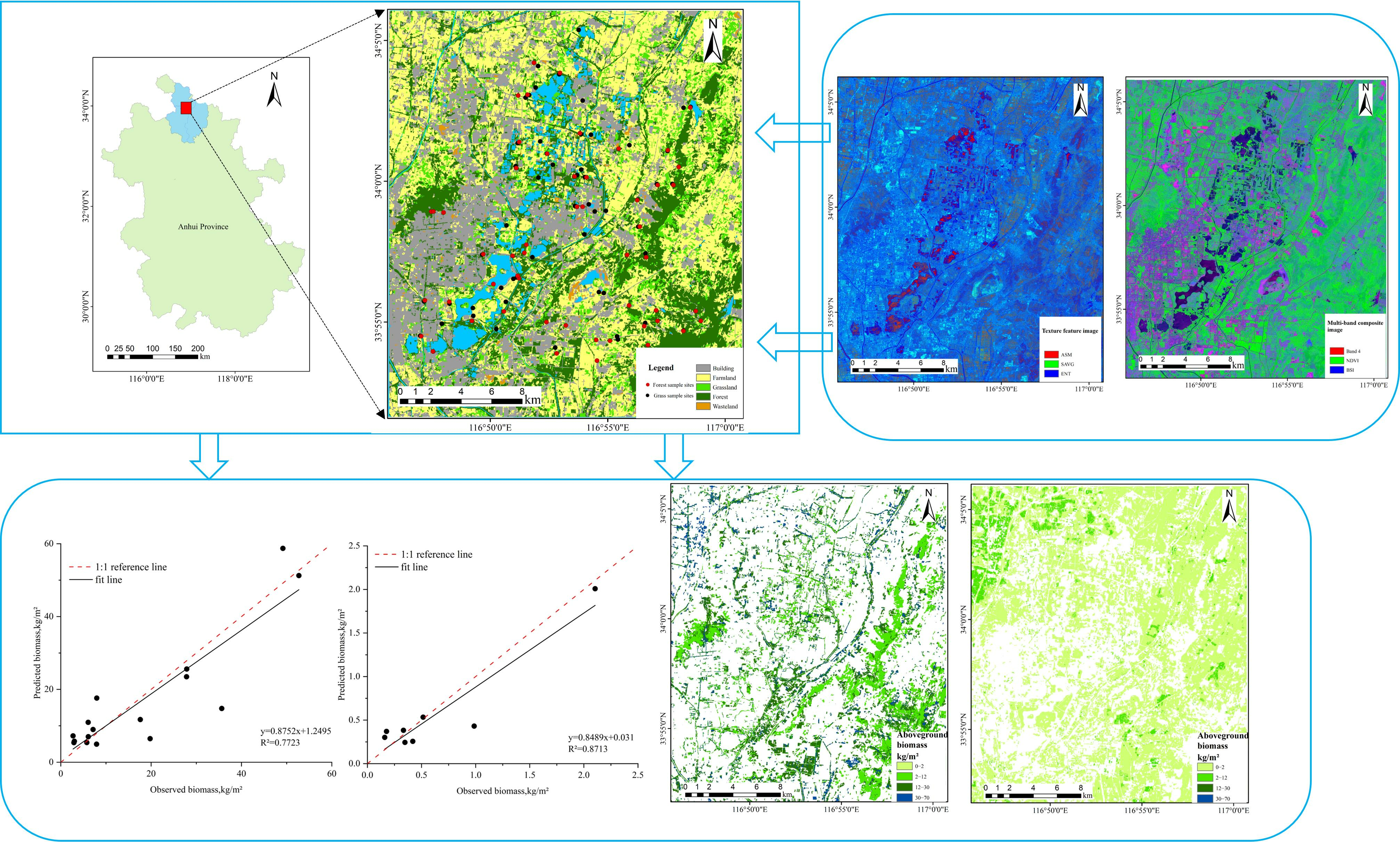
2.1. Overview of the Study Area

The study area is located in Zhahe Mining Area (116°23′E–117°02′E, 33°16′N–34°14′N) between the east side of Xiangshan Mountain and the west side of Longji Mountain in Huaibei City, northern Anhui Province, with the terrain tilted from northwest to southeast and the terrain is relatively flat, which belongs to the warm temperate zone with a semi-moist monsoon climate, with four distinctive seasons, cold winters, hot summers, and the precipitation concentrating in the summer and autumn. The multi-year average precipitation is 816.7 mm [14]. The study area is rich in mineral resources, dominated by coal, natural gas, iron ore, limestone, and kaolin. Among them, coal resources are the richest, and coal mining is mainly underground, and the coal mining area accounts for more than 70% of the urban area of the study area [15]; Figure 1 shows the distribution of the study area and the AGB sampling sites.

2.2. Data Acquisition and Pre-Processing

2.2.1. Sampling for Field Survey

Field sampling was conducted in the study area from 12 to 18 July 2023, with a total of 88 sampling points, including 52 forest sampling points and 36 grass and crop sampling points. The grass and crop samples collected during the sampling process were herbaceous plants. Considering that insufficient data for a single category may result in overfitting issues for the model, the sampled data for grass and crops were combined and collectively referred to as agri-grass data in order to participate in the subsequent AGB inversion modelling calculations.

During the sampling process, precise positioning is conducted for each sampling point to obtain the latitude and longitude coordinates of each point. Three sample squares (0.5 m × 0.5 m) were set up in each agri-grass sampling site. All the vegetation samples above the ground surface in the sample squares were harvested and the fresh weight was measured with a balance with an accuracy of 0.01 g, and then sealed and stored in a kraft paper bag; the samples were dried in the laboratory for 24 h using a constant temperature-drying oven at 85 °C. The samples were taken out for cooling for 10 min and then weighed to determine the dry weights. Subsequently, the data were converted to represent the agri-grass AGB of the sample site within a 10 m × 10 m area. For each forest sampling point, one forest survey plot (15 m × 15 m) and three agri-grass survey plots (0.5 m × 0.5 m) are established. Within the forest plot, detailed records are made of the dominant tree species, the diameter at breast height (DBH) of representative trees, canopy height, and crown radii in both the north–south and east–west directions. The forest AGB within each plot is computed using the allometric growth equations specific to different tree species in the study area, as outlined in

Table 1. AGB calculation formula for different tree species in the study area.

Serial Number	Tree Species	Calculation Formula		Reference
1	Ginkgo biloba	$W_S=0.96\times {(D^{2}H)}^{0.1114}$	$W_B=0.96\times {(D^{2}H)}^{0.0193}$	[15]
		$W_L=0.98\times {(D^{2}H)}^{0.0159}$	$W_T=W_S+W_B+W_L$
2	Populus	$W_S=0.98\times {(D^{2}H)}^{0.0635}$	$W_B=0.98\times {(D^{2}H)}^{0.171}$
		$W_L=0.99\times {(D^{2}H)}^{0.0568}$	$W_T=W_S+W_B+W_L$
3	Koelreuteria paniculata	$W_S=0.88\times {(D^{2}H)}^{0.011}$	$W_B=0.89\times {(D^{2}H)}^{0.0005}$
		$W_L=0.97\times {(D^{2}H)}^{0.00003}$	$W_T=W_S+W_B+W_L$
4	Ligustrum lucidum	$W_S=0.1833\times {(D^{2}H)}^{0.6504}$	$W_B=0.0972\times {(D^{2}H)}^{0.6441}$
		$W_L=0.1495\times {(D^{2}H)}^{0.5085}$	$W_T=W_S+W_B+W_L$
5	Pinus	$W_S=0.0237\times {(D^{2}H)}^{1.0015}$	$W_B=0.0016\times {(D^{2}H)}^{1.1628}$
		$W_L=0.0017\times {(D^{2}H)}^{1.0033}$	$W_T=W_S+W_B+W_L$
6	Other Broadleaved Forests	$W_S=0.045\times {(D^{2}H)}^{0.874}$	$W_B=0.02\times {(D^{2}H)}^{0.839}$
		$W_L=0.01\times {(D^{2}H)}^{0.78}$	$W_T=W_S+W_B+W_L$

Note: W_S is stem AGB, W_B is branch AGB, W_L is leaf AGB, W_L is above ground AGB, D is diameter at breast height, H is tree height.

.

Simultaneously, the agri-grass AGB is determined through the harvest–drying–weighing method. The fresh weight is measured with a precision of 0.01 g using a scale, and the samples are then sealed in paper bags for preservation. The corresponding areas of forest AGB and agri-grass AGB are then aggregated, adjusted to a 10 m × 10 m scale, and subsequently utilized for the computation of the forest AGB at the specific sampling point.

2.2.2. Remote Sensing Image Data

The satellite remote sensing images used are Sentinel-2 and Landsat-8 OLI/TIRS data. The Sentinel-2 remote sensing data are from the GEE platform. The imaging date was 8 July 2023. They data are L2A class data, which have been processed using orthorectification, geometrical refinement correction, and atmospheric correction. The Sentinel-2 L2A image has a spatial resolution of 10 m. It is cropped and resampled to a 10 m resolution on the GEE platform based on the imaging time and the study area’s extent. Additionally, the Sentinel-2 image is further processed on the GEE platform, considering factors such as cloudiness; the Landsat-8 OLI/TIRS image data were obtained from the U.S. Geological Survey (USGS). The image with suitable cloud cover and the nearest capture time to the sampling time (5 August 2023) was selected. The processing level is L1TP, and Landsat-8 OLI/TIRS data consist of 11 bands with a 30 m spatial resolution; the data are resampled to a 10 m spatial resolution.

2.2.3. DEM Data

The DEM data use the Copernicus Digital Elevation Model (COP-DEM) published by the European Space Agency with a spatial resolution of 30 m; the data are resampled to 10 m to make the spatial resolution consistent with the Sentinel-2 data.

2.2.4. Calculation of Feature Variables

Based on the results of the existing literature and multi-band operation parameters, 487 feature variables were constructed, including the band combination operation parameters, vegetation index, terrain parameters, texture characteristics, and vegetation physiological parameters. Notably, not all 487 variables were utilized in the modeling process; some variables were filtered out in subsequent steps. Among them, the band combination operation parameters, vegetation index, texture characteristics, and some vegetation physiological parameters were calculated from the Sentinel-2 data; the terrain parameters were calculated from the DEM data. Land surface temperatures (LSTs) were calculated based on the Landsat8 OLI/TIRS image using a radiative transfer model [16]. Net Primary Productivity (NPP) values were calculated from the improved CASA model using meteorological data, Sentinel-2 data, and land cover classification data. The other vegetation physiological parameters were calculated based on Sentinel-2 data [17]. The Gray-Level Co-occurrence Matrix (GLCM) was calculated from the B3, B4, and B8 bands of the Sentinel-2 data [18].

Table 2. Calculation formulae for the main feature variables.

Parameter Type	Parameter Name	Definition
Multi-band Operation Parameters	Band Addition	$\mathrm{B}i+\mathrm{B}j$
	Band Subtraction	$\mathrm{B}i-\mathrm{B}j$
	Band Multiplication	$\mathrm{B}i·\mathrm{B}j$
	Band Division	$\mathrm{B}i/\mathrm{B}j$
	Difference Ratio Sum	$\left(\mathrm{B}i+\mathrm{B}j\right)/\left(\mathrm{B}i-\mathrm{B}j\right)$
	SumRatio Difference	$\left(\mathrm{B}i-\mathrm{B}j\right)/\left(\mathrm{B}i+\mathrm{B}j\right)$
Vegetation Indices	Normalized Difference Vegetation Index (NDVI)	$\begin{array}{l}\left(\mathrm{B}8-\mathrm{B}4\right)/\left(\mathrm{B}8+\mathrm{B}4\right)\hfill \end{array}$
	Enhanced Vegetation Index (EVI)	$2.5\times (\mathrm{B}8-\mathrm{B}4)/(\mathrm{B}8+6.0\times \mathrm{B}4-7.5\times \mathrm{B}3+1)$
	Normalized Difference Greenness Red Index (NGRVI)	$(\mathrm{B}3-\mathrm{B}4)/(\mathrm{B}3+\mathrm{B}4)$
	Canopy Chlorophyll Content Index (CCCI)	$\left(\left(\mathrm{B}8-\mathrm{B}5\right)/\left(\mathrm{B}8+\mathrm{B}5\right)\right)/\left(\left(\mathrm{B}8-\mathrm{B}4\right)/\left(\mathrm{B}8+\mathrm{B}4\right)\right)$
	Global Vegetation Moisture Index (GVMI)	$\left(\left(\mathrm{B}8+0.1\right)-\left(\mathrm{B}5+0.02\right)\right)/\left(\left(\mathrm{B}8+0.1\right)+\left(\mathrm{B}5+0.02\right)\right)$
	MERIS Terrestrial Chlorophyll Index (MTCI)	$(\mathrm{B}8-\mathrm{B}5)/(\mathrm{B}5-\mathrm{B}4)$
	Normalized Difference Greenness Red-edge Index (NGRVIreg)	$(\mathrm{B}3-\mathrm{B}5)/(\mathrm{B}3+\mathrm{B}5)$
	Modified Nonlinear Vegetation Index (MNLI)	$1.5(\mathrm{B}{8}^2-\mathrm{B}3)/(\mathrm{B}{8}^2+\mathrm{B}3+0.5)$
	Chlorophyll Absorption Ratio Index (CARI)	$\left|a·\mathrm{B}4+\mathrm{B}4+b\right|/\sqrt{a^2+1},a=(b5-b3)/150,b=(1-a)\mathrm{B}3$
Terrain Parameters	Elevation	Elevation(m)
	Slope	Slope (°)
	Topographic Wetness Index (TWI)	$\ln (a/\tan (slope))$
Textural Features	Angular Second Moment (ASM)	${\displaystyle \sum _i{\displaystyle \sum _{j}P{(i,j)}^2}}$
	Entropy (ENT)	$-{\displaystyle \sum _i{\displaystyle \sum _{j}p(i,j)\log (p(i,j)}})$
	Sum Average (SAVG)	${\displaystyle {\sum }_{i=2}^{2N_g}i·P_{x+y}(i)}$$, N_g$ is the number of grayscale levels in the $\mathrm{image}, P_{x+y}(i)$ represents the probability that the sum of pixelpairs in the Gray-Level Co-occurrence Matrix (GLCM) is i
VegetationPhysiologicalParameters	Fraction of Photosynthetically Active Radiation (FPAR)	Proportion of photosynthetically active radiation absorbed by the vegetation canopy
	Chlorophyll Content in the Leaf (CAB)	Vegetation leaf chlorophyll content
	Net Primary Productivity (NPP)	The net amount of light energy absorbed by a plant during photosynthesis
	Canopy Water Content (CWC)	Vegetation canopy water content
	Fraction of Vegetation Cover (FVC)	$(\mathrm{N}\mathrm{D}\mathrm{V}\mathrm{I}-\mathrm{N}\mathrm{D}\mathrm{V}{\mathrm{I}}_{\mathrm{s}\mathrm{o}\mathrm{i}\mathrm{l}})/(\mathrm{N}\mathrm{D}\mathrm{V}{\mathrm{I}}_{\mathrm{v}\mathrm{e}\mathrm{g}}-\mathrm{N}\mathrm{D}\mathrm{V}{\mathrm{I}}_{\mathrm{s}\mathrm{o}\mathrm{i}\mathrm{l}})$
	Land Surface Temperature (LST)	Surface temperature (°C)

Note: B_i, B_j are different bands of the Sentinel-2 image. LST parameters were calculated using Landsat-8 TIRS data.

shows the formulas for some of the main feature variables.

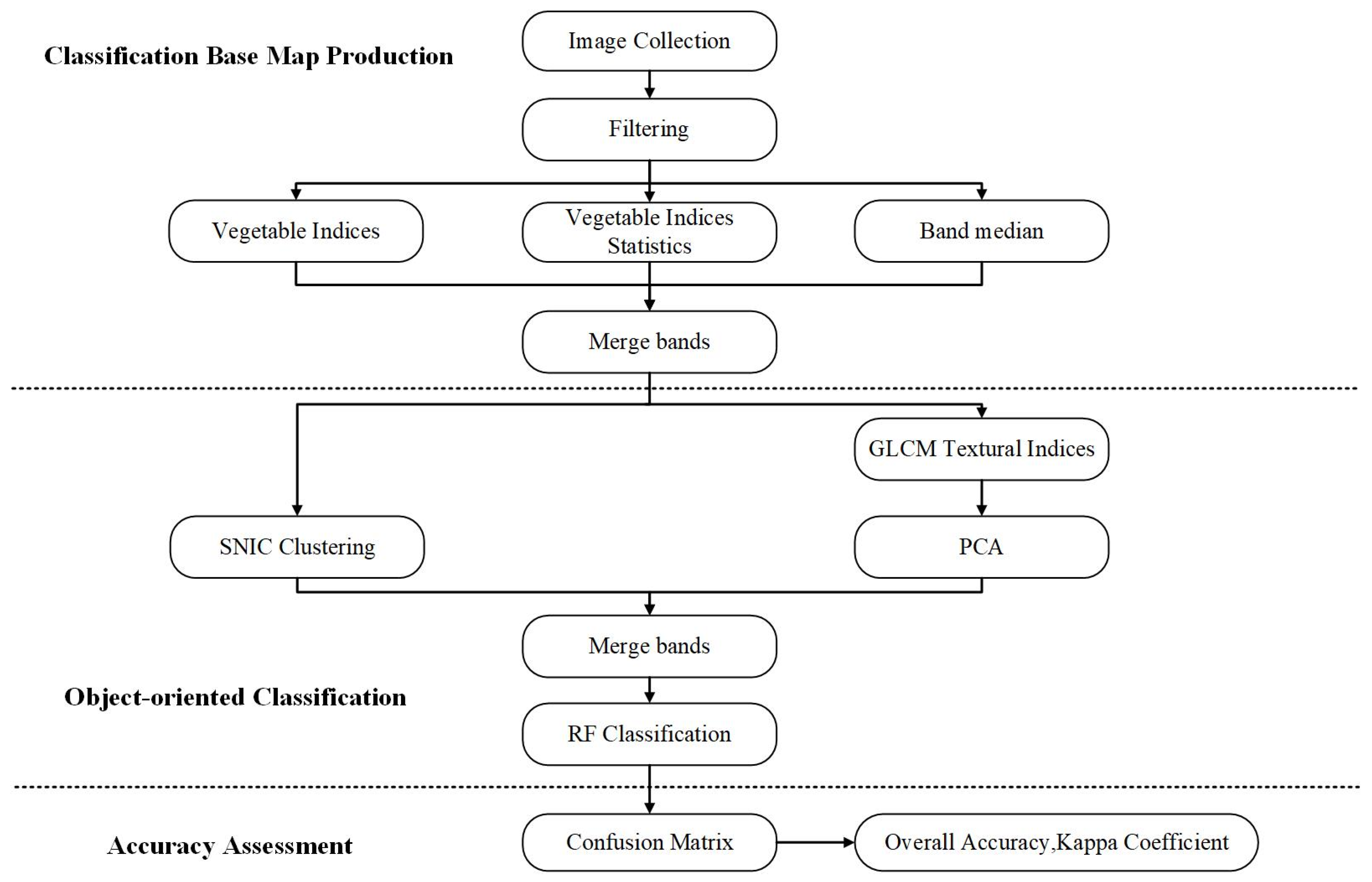
2.3. Object-Oriented Supervised Classification Algorithm

The object-oriented machine learning classification algorithm combining Simple Non-Iterative Clustering (SNIC) and GLCM features was used on the GEE platform to classify the study area features into water bodies, construction land, grassland, cultivated land, forest land, and bare land, and the workflow is shown in Figure 2. Prior to classification, preprocessing was applied to the Sentinel-2 images. Given that the Normalized Difference Vegetation Index (NDVI) effectively highlights differences between vegetated and non-vegetated areas [19,20], and the Bare Soil Index (BSI) is more effective in distinguishing between arable land and bare land [21], the single-band data were processed, the BSI and statistical data (minimum, maximum, standard deviation) of the BSI were merged into the same layer to generate the classification base map. Relying on the ArcMap processing system to produce training data, and the feature type data obtained from the field survey were used as validation data. The training dataset comprised 264 points, while the validation dataset consisted of 100 points.

Next, spatial clustering and texture information calculation were performed using the SNIC clustering algorithm to classify similar and continuous pixels into a group, using the grey scale covariance matrix to calculate texture features based on the classification base map, and standardizing the data to obtain the first principal component (PC1), which contains most of the texture information, through Principal Component Analysis (PCA). The PC1 mean value of each object included in the clusters was calculated to reflect the texture features of that object. Then, they were combined with the bands generated with SNIC clustering to create a dataset that contains both texture information and SNIC clustering information.

Finally, the trained random forest classifier was combined with texture information and clustering details to achieve land cover classification using an object-oriented approach. The confusion matrix was calculated using both the training and validation set data to further evaluate the classification accuracy.

2.4. AGB Inversion Techniques

2.4.1. Machine Learning Algorithm Models

In order to find the optimal AGB machine learning inversion model, nine machine learning regression algorithms and models are constructed for forest and agri-grass AGB inversion in the study area.

(1)

SV-R. The support vector regression (SV-R) model is a machine learning model for regression prediction of data, which is based on the principle of using a kernel function to map the input data into a high dimensional space, and to find a hyperplane in the high dimensional space that is closest to the sample data, in order to minimize the error between predicted and true values, and then to achieve high precision regression prediction [22].Compared with the ordinary linear model, it can better deal with nonlinear relationships and has a strong generalization ability to high dimensional data.

(2)

RF-R. The random forest regression (RF-R) algorithm is an integrated learning algorithm based on decision tree regression, which improves the performance and generalization ability of the model by integrating the prediction results from multiple decision trees [23]. Self-sampling and random feature selection are performed on the training sample data to generate multiple decision trees, and the final regression results are obtained by taking a weighted average of the prediction results of multiple decision trees.

(3)

XGBoost-R. The extreme gradient boosting regression (XGBoost-R) algorithm is a machine learning algorithm based on gradient-boost decision tree (GBDT); XGBoost is similar to GBDT and belongs to the gradient-boosting algorithm, which iteratively trains the decision tree to improve the accuracy of prediction results. However, unlike GBDT, XGBoost uses a second-order Taylor expansion to optimize the loss function, and a regularization term is added to the objective function to control the complexity of the model. The XGBoost model is the result of the integration of multiple weak learners, each of which fits the residuals of the previous one to improve the model accuracy through multiple rounds of iterations [24].

(4)

KNN-R. The core of the K-Nearest Neighbor Regression (KNN-R) algorithm is to achieve regression prediction by measuring the distance between sample data. Based on the calculated distance, the k feature data closest to the new sample data are selected, and the selected k feature data take the weighted average as the prediction data [25].

(5)

LWL-R. The Locally Weighted Linear Regression (LWL-R) algorithm is based on the introduction of a kernel function, which assigns a higher weight to the training data that are closest to the predicted data by calculating the distance between the training data and the target data [26]. The weights need to be recalculated for calculating each training data, and a weighted least squares model combined with a weight matrix is used to fit a local linear model to the predicted data.

(6)

Ridge-R. The Ridge Regression (Ridge-R) model is an improved linear regression model, which introduces an L2 van regularization term in the cost function to prevent overfitting as well as to improve the generalization of the model as compared to ordinary linear regression models [27]. The Ridge-R algorithm works better when the degree of feature covariance is high.

(7)

PLS-R. The Partial Least Squares Regression (PLS-R) model is suitable for scenarios where there are multiple correlations between variables and less modelling data; unlike a traditional regression model, which directly fits the training data to the predicted data, the PLS-R model reduces the dimensionality of the data by searching for the least squares variables to build the regression model [28].

(8)

Poly-R. The Polynomial Regression (Poly-R) modelling idea is more similar to ordinary linear regression; both directly use training data to fit predicted data. However, the Poly-R model also introduces higher powers of the training features, which makes the data dimensionality increase and builds a model that can better fit the nonlinear data [29].

(9)

Enet-R. The Elastic-net Regression (Enet-R) algorithm incorporates Lasso regression and Ridge-R regularization methods. L1 regularization and L2 regularization are introduced to control model complexity, handle covariance features, and find a balance between feature selection and model stability [30].

2.4.2. Feature Selection Algorithm

In order to eliminate redundant features and identify the optimal subset that enhances model inversion accuracy, we employ the Pearson correlation coefficient and the minimum redundancy maximum relevance (mRMR) algorithms for the optimal selection of feature variables.

(1)

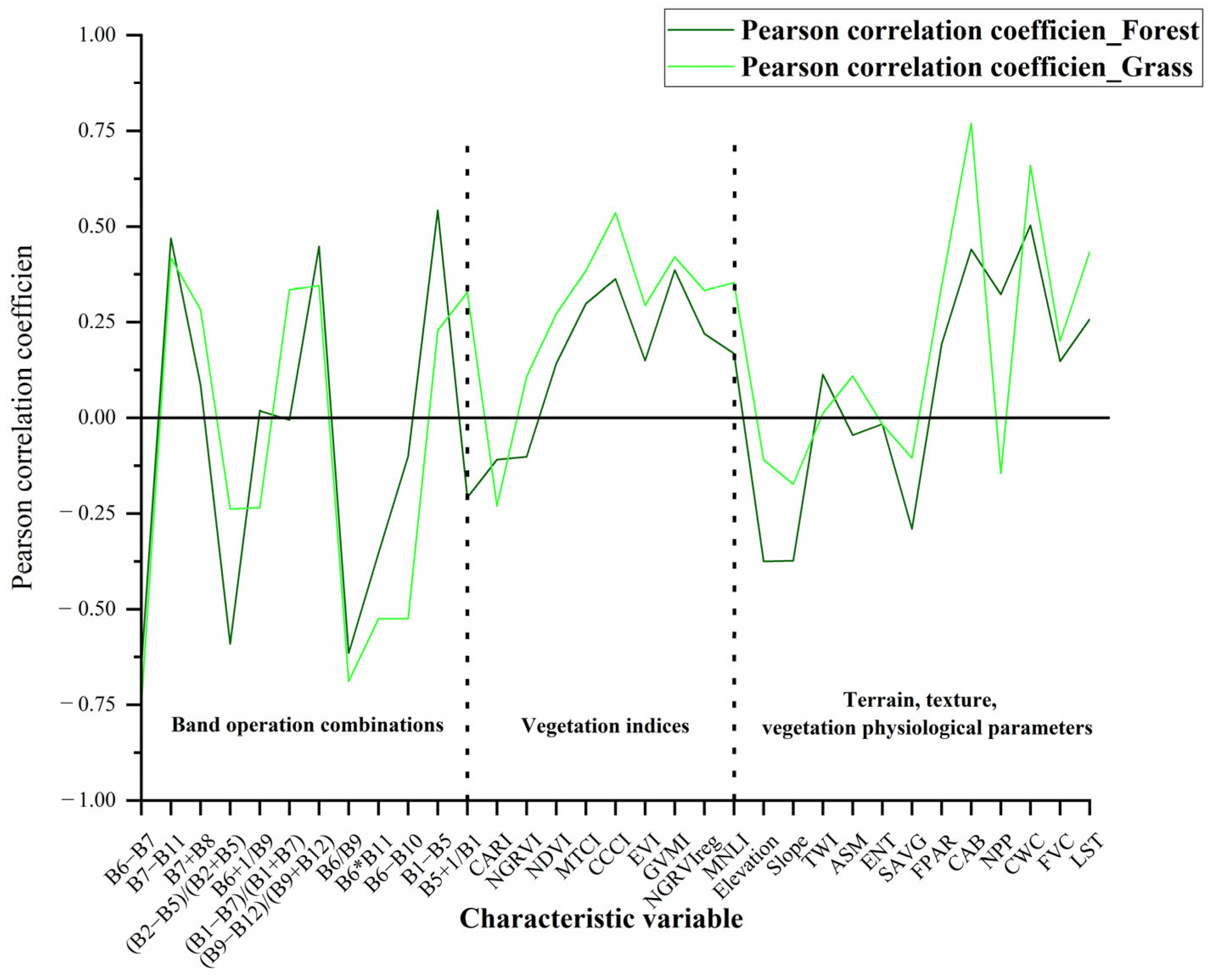
Pearson correlation coefficient (r). The Pearson correlation coefficient can be used to assess the correlation between each feature variable and the measured real measurements, calculated as follows:

$$r=\frac{{\displaystyle \sum (X_i-\overline{X})(Y_i-\overline{Y})}}{\sqrt{{\displaystyle \sum {(X_i-\overline{X})}^2{\displaystyle \sum {(Y_i-\overline{Y})}^2}}}}$$

(1)

where X_i and Y_i are the corresponding feature variables and real measurement data of the sampling points, $\overline{X}$ and $\overline{Y}$ are the mean value of the feature variables and the mean value of the real measurements of the sampling points, and the correlation coefficients take the values between −1 and 1; a larger absolute value represents a stronger correlation between the two variables [31].

(2)

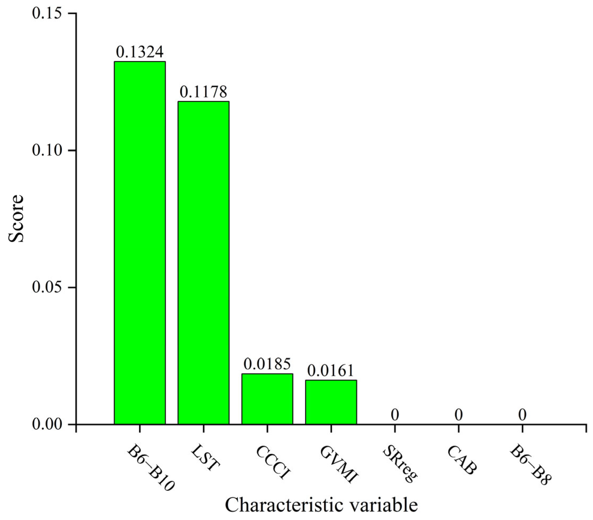
mRMR feature selection method. The mRMR algorithm’s core is to increase the correlation between feature variables and targets while reducing the redundancy between feature variables [32]. Using mutual information as a measure of correlation between feature variables, the mutual information between feature variables can be calculated using the following equation.

$$I(x,y)={\displaystyle \sum _{i,j}p(x_i,y_j)\log \frac{p(x_i,y_j)}{p(x_i)p(y_j)}}$$

(2)

where p(x,y) is the joint probability density between two variables, and p(x), p(y) are the marginal probabilities of two variables, respectively. According to Equation (2), the screening condition for the minimum redundant subset is as follows:

$$W_I=\frac{1}{{\left|S\right|}^2}{\displaystyle \sum _{i,j\in S}I(g_i,g_j)},\min W_I$$

(3)

where S is the feature subset, |S| is the number of features in the subset, and g_i, g_j are different feature variables. In order to maximize the correlation between the subset feature variables and the target, the feature subset needs to satisfy the following conditions:

$$V_I=\frac{1}{\left|S\right|}{\displaystyle \sum _{i\in S}I(h,g_i),\max V_I}$$

(4)

where h is the target feature. mRMR algorithm’s final criterion is a linear combination of maximizing relevance and minimizing redundancy, denoted as:

$$mRMR=V_I-\lambda W_I$$

(5)

where λ is a regulation parameter to balance the weight of correlation combined redundancy.

In the study area, after calculating the Pearson correlation coefficient of all 487 feature variables and removing the autocorrelation variables, the mRMR feature selection algorithm was used to select the remaining feature variables based on the rankings of the feature variable scores, and six forest AGB modelling features and four agri-grass AGB modelling features were finally screened out.

2.4.3. PmM Model for AGB Remote Sensing Inversion

Using the Pearson–mRMR feature variable optimal screening algorithm, the optimal screening of the study area band combination operation parameters, vegetation indices, terrain parameters, texture features, and vegetation physiological parameters, using SV-R, RF-R, XGBoost-R, KNN-R, LWL-R, Ridge-R, PLS-R, Poly-R, and Enet-R machine learning (ML) algorithms and models, were combined with the screened model application feature variables to construct the Pearson–mRMR–machine learning (PmM) model for optimal forest and agri-grass AGB inversion in the study area. The technical route of the PmM model for the remote sensing inversion of AGB is shown in Figure 3.

(1)

Firstly, apply the object-oriented machine learning algorithm on GEE to classify the features in the study area, obtaining high accuracy distribution maps for forests and agri-grasses;

(2)

Then, calculate the combination data of the number of bands, vegetation indices, topographic data, texture characteristics, and physiological parameters of vegetation in the study area, and use the drying–weighing method to obtain the agri-grass AGB data, and use the heterogeneous growth equation to obtain the forest AGB data;

(3)

Preliminarily screen the feature variables with high correlation with measured AGB data of forest and agri-grass using Pearson correlation coefficient, and further screen the screened feature variables using the mRMR algorithm to obtain feature variables for final inverse modelling and application of forest and agri-grass, respectively;

(4)

Divide the sample dataset. Set the ratio of the training set and validation to 8:2 for both forest and agri-grass samples. Set the parameters according to the characteristics of each machine learning algorithm. Evaluate the models using the training set R², validation set R², and root mean square error RMSE.

(5)

Select the optimal machine learning model to map the distribution of forest and agri-grass AGB in the study area.

2.4.4. AGB Inversion Model Accuracy Assessment Methods

(1)

Data input and model parameter adjustment

Input the characteristic variables of forests and agricultural grasses into the AGB inversion model, respectively, adjust the model parameters by considering the model characteristics and incorporating a priori experience during modeling. Obtain optimal parameters based on each evaluation index.

(2)

Evaluation of model accuracy

After the establishment of machine learning models for forests and agricultural grasses in the study area, the coefficient of determination (R²), the root mean square error (RMSE), and the mean absolute error (MAE) were used to compare the gap between the predicted data and the measured data of each model. The formulas were calculated as follows:

$$R_{train}^2=1-\frac{{\displaystyle \sum _{i=1}^n{(y_{train,i}-{\widehat{y}}_{train,i})}^2}}{{\displaystyle \sum _{i=1}^n{(y_{train,i}-{\overline{y}}_{train,i})}^2}}$$

(6)

where n is the number of samples in the training set, $y_{train,i}$ is the actual value of the ith sample in the training set, ${\widehat{y}}_{train,i}$ is the predicted data of the ith sample in the training set, and ${\overline{y}}_{train,i}$ is the mean value of the measured data of the samples in the training set.

The validation set was calculated as follows:

$$R_{val}^2=1-\frac{{\displaystyle \sum _{i=1}^m{(y_{val,i}-{\widehat{y}}_{val,i})}^2}}{{\displaystyle \sum _{i=1}^m{(y_{val,i}-{\overline{y}}_{val,i})}^2}}$$

(7)

$$RMS{E}_{val}=\sqrt{\frac{1}{m}{\displaystyle \sum _{i=1}^m{(y_{val,i}-{\widehat{y}}_{val,i})}^2}}$$

(8)

$$MA{E}_{val}=\frac{1}{m}{\displaystyle \sum _{i=1}^m\left|y_{val,i}-{\widehat{y}}_{val,i}\right|}$$

(9)

where m is the number of samples in the validation set, $y_{val,i}$ is the actual value of the ith sample in the validation set, ${\widehat{y}}_{val,i}$ is the predicted data for the ith sample in the validation set, and ${\overline{y}}_{val,i}$ is the mean value of all the measured sample data in the validation set.

3. Results

3.1. The Measured AGB of Different Vegetation Cover Types

The statistical results of the measured forest and agri-grass AGB are presented in

Table 3. Measured AGB data in the study area.

	Maximum Value (kg/m2)	Minimum Value (kg/m2)	Average Value (kg/m2)
Observed Forest AGB	84.27	2.11	17.77
Observed Grass AGB	5.27	0.10	0.61

. The estimation results reveal that the AGB of agri-grass varies from 0.10 to 2.10 kg/m², with a mean value of 0.48 kg/m². The majority of agri-grass samples exhibit a comparatively lower AGB, and overall, the distribution of agri-grass AGB is narrow, with most samples concentrated at lower levels. In contrast, the AGB of forests ranges from 2.11 to 84.27 kg/m², with a mean value of 17.77 kg/m². Forests generally demonstrate higher AGB, and the mean value is significantly greater than that of agri-grass AGB. This difference may be attributed to variations in growth environments and tree species, with some sampling points in forests showing a notably low AGB.

3.2. Feature Classification Results and Accuracy Evaluation

Figure 4 displays the outcomes of the random forest feature classification, combining texture information and a simple clustering method. The features in the study area primarily include water bodies, construction land, arable land, grassland, forest land, and unused land. Notably, the construction area exhibits a higher density and a larger range of water bodies, while forests and agri-grasses are predominantly distributed along water systems and mountain ranges. Arable land, on the other hand, has the widest distribution range in the study area.

Figure 5 shows a comparison of the accuracy of the two classification methods, with an overall classification accuracy of 88% and a Kappa coefficient of 84% for the pixel-based classification method. These results indicate that the feature classification method used in this study is more effective in extracting the distribution of forests and agricultural grasslands.

3.3. Feature Correlation Analysis and Feature Selection Results

Figure 6 shows the Pearson correlation between the calculated feature variables of forest and agri-grass and the corresponding measured AGB. On the whole, the AGB of forests and agricultural grasses has a better correlation with the feature variables, higher correlation with some parameters of the band combination operation, poorer correlation with some texture features, positive correlation with most of the vegetation indices and vegetation physiological parameters, and negative correlation with terrain parameters; for the same feature variable, the correlation coefficients between the feature variables corresponding to different vegetation cover types and the measured AGB do not significantly differ. Specific analyses showed that for forest AGB data, band combination parameters (B6 − B7, (B2 − B5)/(B2 + B5), B6/B9, B7 − B11, (B9 − B12)/(B9 + B12), B1 − B5), vegetation indices (MTCI, CCCI, GVMI), topographic parameters (Elevation, Slope), texture features (SAVG), and vegetation physiological parameters (CAB, CWC) were highly correlated with the measured AGB; for agri-grass data, the band combination data B6 − B7, B7 − B11, B6/B9, B6 × B11, B6 − B10, the vegetation indices MTCI, CCCI, GVMI, NGRVI_reg, and MNLI, and the vegetation physiological parameters FPAR, CAB, CWC, and LST showed a strong correlation with the measured agri-grass AGB data, and topographic data and textural data showed a low correlation with the agri-grass AGB data.

Figure 7 and Figure 8 illustrate the mRMR screening outcomes for forest and agri-grass feature variables. In the case of forest modeling, the features were ranked based on their mRMR scores in descending order, with the top-ranking features being B6 − B7, CCCI, B1 − B5, DEM, B5 + 1/B1, Slope, B6 + 1/B7, and B5 + 1/B2. However, the scores of B6 + 1/B7, B5 + 1/B2, and NPP were all 0, indicating they did not meet the criteria of high relevance and low redundancy. Therefore, the top six features with the highest scores were selected as the final variables for modeling. For agri-grass modeling, B6 − B10 and LST received high mRMR scores, suggesting a strong correlation with the target variables and minimal redundancy among features. Despite lower scores, CCCI and GVMI were also included in the modeling to prevent underfitting due to a limited number of variables. As a result, the modeling features for agri-grass comprised band combination parameters B6 − B10, vegetation indices CCCI and GVMI, along with the vegetation physiological parameter LST.

3.4. Modelling Results

3.4.1. Forest AGB Inversion Model and Validation

Forest modeling features are extracted from the remote sensing image for each sampling point based on their coordinates. These features are then combined with the measured AGB data to establish a machine learning estimation model for forest AGB. The AGB modeling data, consisting of 52 sets, were divided into two groups: 36 for model construction and 16 for model validation. As can be seen from Figure 9, the R² of the validation dataset exhibits that the LWL-R model < RF-R model, and the R² of the validation set of the training set of the RF-R model and the LWL-R model is higher. Both of them reach more than 0.7, with a better model generalization ability, and there is a more serious overfitting phenomenon in the XGBoost-R model; the RMSE of the validation set exhibits that the RF-R model < LWL-R model, and the MAE from low to high is LWL-R model < RF-R model; the training set R² of RF-R model reaches 0.91, while the validation set R² is 0.77, the validation set RMSE is 5.21 kg/m², and the validation set MAE is 9.28 kg/m². The simulated AGB and the measured AGB are used to validate the identified best forest AGB model (Figure 10), and the slope of the linear regression formula reaches 0.8752. The comprehensive multi-indicator analysis showed that the RF-R model has high accuracy and stability, and the inversion values can fit the measured results better, so the RF-R model is optimal for estimating the forest AGB.

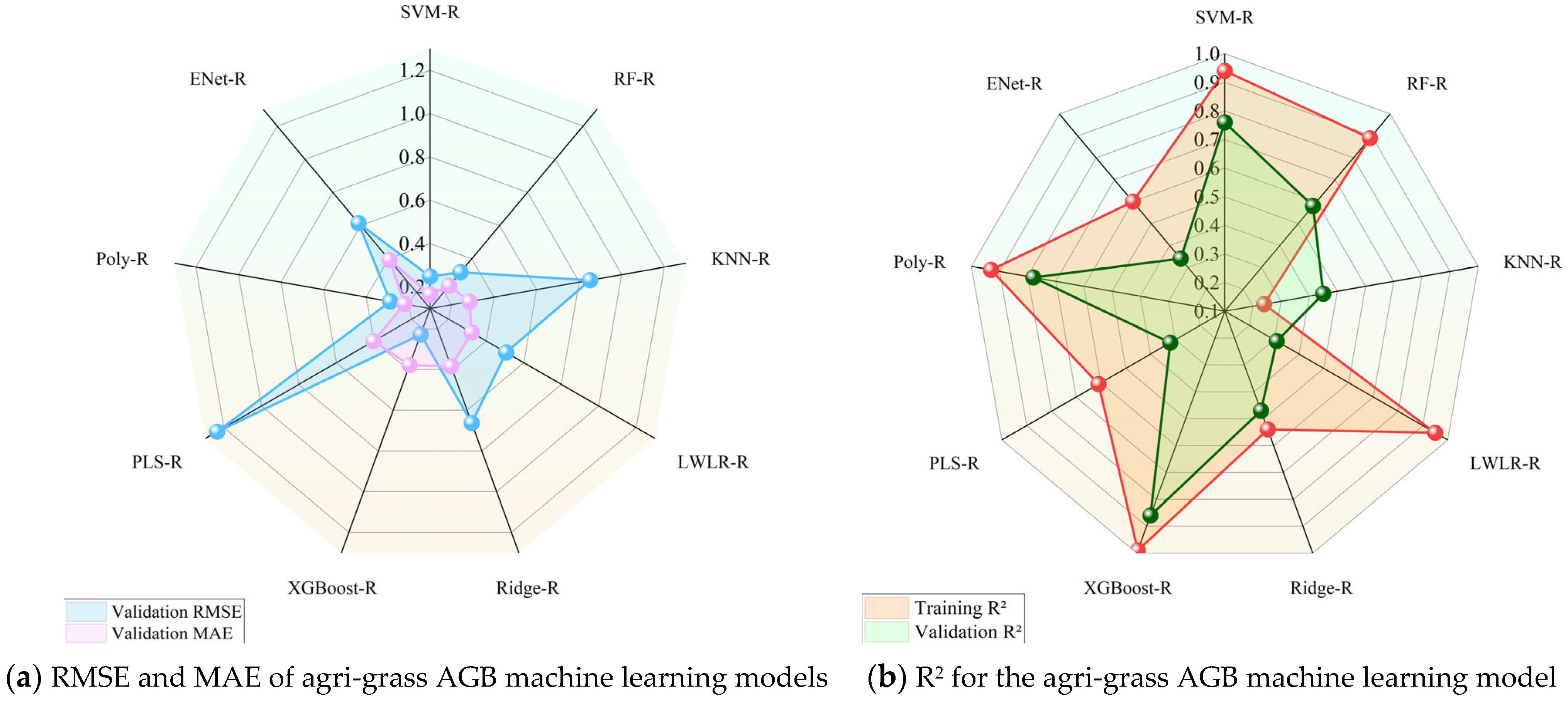
3.4.2. AGB Inversion Model and Validation on Agri-Grass Land

The features for agri-grass modeling were extracted using the coordinates of the agri-grass sampling points and were combined with 28 sets of measured agri-grass AGB data to establish a machine learning estimation model for agri-grass AGB. Additionally, eight sets of measured AGB data were reserved for validation purposes. As depicted in Figure 11, the modeling accuracy of the XGBoost-R, Poly-R, and SV-R models is high, with the R² of both the training and validation sets exceeding 0.7. Notably, the R² of the validation set is ranked in the following order: Poly-R < SV-R < XGBoost-R. Similarly, the RMSE of the validation set is ordered as follows: XGBoost-R < SV-R < Poly-R; the MAE is ordered as follows: SV-R < Poly-R < XGBoost-R. Compared with other machine learning models, the XGBoost-R model has the highest validation set R² and the lowest validation set RMSE, which are 0.86 and 0.23 kg/m², respectively. Figure 12 illustrates the accuracy results of the best agri-grass AGB model, with the slope of the linear regression formula reaching 0.8489. The agri-grass AGB inversion results exhibit high consistency with the measured values, indicating optimal model performance.

3.5. AGB Distribution in the Study Area

The established RF-R and XGBoost-R models were employed to estimate the aboveground biomass (AGB) of forests and grasslands in the study area, respectively. The combined results of forest and grassland AGB estimation are illustrated in Figure 13. The inversion results reveal that the predicted AGB values for forests in the study area range from 0 to 69 kg/m², with an average of 4.60 kg/m². On the other hand, the predicted AGB values for grasslands in the study area range from 0 to 5.26 kg/m², with an average of 0.71 kg/m². The spatial distribution of AGB demonstrates significant variability across the study area, with high AGB values predominantly concentrated along the western Xiangshan Mountain and the eastern Longji Mountain areas, ranging between 2 kg/m² and 12 kg/m²; this observation aligns with the vegetation distribution depicted in Figure 13 and the landcover classification shown in Figure 4, indicating that forests mainly cover these areas. Notably, elevated AGB values (12–30 kg/m²) are observed along road networks and water systems, where tall trees like poplar and pine trees are frequently found. This distribution leads to abrupt increases in local AGB values. Additionally, the AGB of the ecological restoration wetland of the South Lake ranges from 0 to 30 kg/m², with an average of 1.4 kg/m², which is significantly higher than that of the surrounding urban areas. This suggests the effectiveness of ecological reclamation efforts in improving the environmental quality of peripheral urban areas and enhancing the urban carbon cycle. Conversely, lower AGB values are observed in farmlands surrounding the town, primarily consisting of herbaceous plants and crops; the AGB of the northwestern cultivated area exceeds 2 kg/m², which is slightly higher than that of other areas also classified as cultivated areas.

It is worth noting that the AGB exceeded 30 kg/m² in some areas, which were mainly located in the northwest and east of the study area, distributed along roads and rivers, as well as Xiang Mountain and Longji Mountain. During field sampling, we found that the areas of high AGB values along the roads and rivers in the northwest were mainly distributed by mature poplar forests, and these trees were generally over 25 m tall with a diameter at DBH of over 80 cm. In contrast, the high value areas of Xiang Mountain are dominated by artificially planted lateral cypresses and cedars, which have a diameter at DBH of more than 100 cm and a tree height of more than 20 meters. In the eastern Longji Mountain, the AGB high value areas are mainly composed of tall cypress trees that grow naturally on the mountain, and these trees are more densely distributed. The existence of these high value areas may be due to the fact that the vegetation types and vegetation structures in these areas are different from those in the surrounding areas, resulting in a significant increase in their AGB values.

4. Discussion

In this study, remote sensing data and derived data, such as band combinations, vegetation indices, textural features, topographic parameters, and vegetation physiological parameters, were used to estimate the AGB in the urban and surrounding areas of the study area. The best independent variables were selected by using correlation coefficients and mutual information. Compared with single type ecosystems such as forest ecosystems and grassland ecosystems, urban areas are more complex in terms of topography and features, and the distribution of vegetation is more fragmented and spatially heterogeneous, so the influence of man-made features on the distribution of AGB must be considered in the estimation of AGB; therefore, more accurate feature classification data are required for the estimation of AGB in urban areas. The accurate identification of boundaries between different feature types significantly impacts AGB inversion [7]. In this study, we use an object-oriented machine learning classification method to achieve an overall classification accuracy of 95%, with a Kappa coefficient of 93%, which is 7% and 10% higher than pixel-based classification methods, respectively. Our method better identifies boundaries between vegetation and non-vegetation areas, as well as between different vegetation types, thereby obtaining more accurate spatial distributions of AGB.

The feature variables were screened by the Pearson–mRMR feature variable preference method, and in this study, we found that the red-edge bands B5 and B6 and the near-red band B8 of the Sentinel-2 image were more correlated with the vegetation AGB than the visible bands, which is similar to the results of Morada et al. [33]. The elevation variable had some effect on forest AGB, probably because the distribution of different tree species in the forest as well as their growth conditions are constrained by climatic conditions such as temperature and precipitation, and elevation affects climate more vertically than horizontally; thus, elevation affects forest AGB to a certain extent [34]. We found that the LST was more important for agri-grass AGB, and a higher surface temperature increased the photosynthetic rate of agri-grass, which in turn positively affected the vegetation growth; John et al. [35]. and Liu et al. [36]. obtained similar results.

This study showed that the RF-R model estimated the urban area forest low AGB with higher accuracy, which is consistent with the findings of Bai et al. [37]. For the agri-grass AGB inversion model, the XGBoost-R model inversion was the best. However, in this study, the forest AGB inversion using the RF-R model suffered from the overestimation of low values and underestimation of high values, and other scholars had the same problem in estimating forest AGB using the RF-R model [38]. The reasons may be that the measured forest AGB values in the study area vary greatly, resulting in the RF-R model being affected by extreme values. Additionally, the heterogeneity of the features in the study area is more obvious. For the areas with low forest AGB values, some forest pixels are affected by the spectra of other features, which are not pure pixels of the forests; therefore, the AGB estimated using the spectral information is higher than the actual value. Conversely, in areas with high forest AGB values, the reflectance spectrum of the vegetation with high forest AGB values are easily saturated, resulting in a slightly lower AGB than the actual AGB for the inverse performances.

In this study, it was found that the predicted agri-grass AGB obtained using the XGBoost-R model was lower than the actual value, which may be due to the fact that the distribution of agri-grass is more sparse, and the reflectance of agri-grass in the image element is interfered by the soil background and the adjacent features, so that the actual reflectance obtained is that of the mixed image element, which in turn leads to the underestimation of the overall agri-grass AGB.

The AGB inversion model, employing the land cover classification feature selection machine learning algorithm, offers several advantages. The precise feature classification results enable the accurate delineation of the boundaries of various vegetation types, facilitating the extraction and modeling of AGB features for different vegetation types. Additionally, the feature extraction algorithm optimizes and filters the acquired feature variables, enhancing the model’s ability to learn the non-linear relationship between variables and predicted features.

However, despite the model’s advantages, certain limitations must be acknowledged. Firstly, due to traffic limitations, sampling points are relatively scarce in the western Xiang Mountain region and the eastern Longji Mountain region, potentially resulting in less accurate AGB estimation in these corresponding regions. Secondly, the machine learning model’s internal mechanism is intricate, making the operation process challenging to control. Thirdly, this study primarily establishes the AGB inversion model for mining urban ecosystems, requiring further validation of the model’s validity and accuracy in other ecosystems.

Estimating AGB in urban ecosystems presents unique challenges, primarily due to the complex feature distribution and human modification of surrounding ecosystems. Large-scale AGB estimation modeling necessitates more field data to enhance the model’s reliability for AGB inversion in various urban ecosystems. Therefore, extensive field data collection is imperative to improve AGB inversion accuracy in urban ecosystems. Besides passive optical, topographic, and meteorological data, utilizing additional field data, such as soil data, can provide insights into the complex relationship between AGB and the environment. Integrating these additional data sources, including vegetation physiological parameters, climate data, and soil data, can further enhance AGB inversion model accuracy and applicability. Additionally, the emergence of deep learning presents opportunities to construct more complex AGB inversion models. Deep learning can extract richer and higher-level features from large datasets, capturing more intricate data relationships [39]. By collecting more comprehensive field data and employing advanced deep learning modeling methods, future research can explore more complex deep learning architectures to better capture non-linear data relationships, enhancing model robustness and generalization. Employing these methodologies can achieve more accurate and comprehensive urban ecosystem AGB inversion, providing effective support for urban ecological environment protection and management, and serving as a reference for urban ecosystem protection and rational forest resource utilization.

5. Conclusions

In this study, we first developed an object-oriented feature classification model using GEE to generate high-precision vegetation distribution maps. Using field measurement data, band combination data, vegetation indices, topographic data, texture features, and vegetation physiological parameters, we constructed nine machine learning models for estimating forest AGB and crop AGB, respectively. Subsequently, the optimal machine learning model was used to generate a spatial distribution map of the AGB in the study area. Our results are as follows:

(1)

The overall classification accuracy and Kappa coefficient of the object-oriented feature classification model are improved by 7% and 9%, respectively, compared with the classification model based on image elements; the object-oriented feature classification model is able to better distinguish between vegetation and non-vegetation as well as the boundaries between different types of vegetation.

(2)

For forest AGB inversion, the RF-R model is more accurate than other machine learning models, with an R² of 0.76 and an RMSE of 5.21 kg/m². For agri-grass AGB inversion, the XGBoost-R model achieved a higher accuracy with an R² of 0.86 and RMSE of 0.23 kg/m². Therefore, RF-R and XGBoost-R models were used to estimate forest and agri-grass AGB in the study area, respectively.

(3)

For forest AGB, the multi-band operation parameters B6 − B7, B1 − B5, B5 + 1/B1, the CCCI, and the topographic parameters elevation and slope were more highly correlated with the forest AGB. For agri-grass AGB, the multi-band operation parameters B6 − B10, the CCCI and GVMI, and vegetation physiological parameter LST were more correlated with grassland AGB.

(4)

The average AGB value was 4.60 kg/m² for forests and 0.71 kg/m² for agricultural grasslands, similar to the results of other studies. The high AGB values in the study area are mainly distributed along the water system, roads, and mountains, and the above areas are mostly distributed with tall perennial trees; lower AGB values are observed in farmlands surrounding the town, primarily consisting of herbaceous plants and crops.

Overall, the AGB distribution mapped by the constructed model is useful for assessing the ecological restoration of the mining area and the sustainable use of forest resources. Future research could address the limitations associated with limited ground reference data by utilizing advanced deep learning techniques and wider datasets to improve the accuracy and applicability of the model.

References

1. Blanco, E.; Pedersen Zari, M.; Raskin, K.; Clergeau, P. Urban Ecosystem-Level Biomimicry and Regenerative Design: Linking Ecosystem Functioning and Urban Built Environments. Sustainability 2021, 13, 404. [Google Scholar] [CrossRef]
2. Li, L.; Zhou, X.; Chen, L.; Chen, L.; Zhang, Y.; Liu, Y. Estimating Urban Vegetation Biomass from Sentinel-2A Image Data. Forests 2020, 11, 125. [Google Scholar] [CrossRef]
3. Yin, K.; Lu, D.; Tian, Y.; Zhao, Q.; Yuan, C. Evaluation of Carbon and Oxygen Balances in Urban Ecosystems Using Land Use/Land Cover and Statistical Data. Sustainability 2014, 7, 195–221. [Google Scholar] [CrossRef]
4. Sullivan, P. Energetic Cities: Energy, Environment and Strategic Thinking. World Policy J. 2010, 27, 11–13. [Google Scholar] [CrossRef]
5. Fang, J.; Wang, Z. Forest biomass estimation at regional and global levels, with special reference to China’s forest biomass. Ecol. Res. 2001, 16, 587–592. [Google Scholar] [CrossRef]
6. Zhang, P.; Liang, Y.; Liu, B.; Ma, T.; Wu, M. Remote sensing estimation of forest aboveground biomass in Tibetan Plateau based on random forest model. Chin. J. Ecol. 2023, 42, 415–424. [Google Scholar] [CrossRef]
7. Sun, S.; Wang, Y.; Song, Z.; Chen, C.; Zhang, Y.; Chen, X.; Chen, W.; Yuan, W.; Wu, X.; Ran, X.; et al. Modelling Aboveground Biomass Carbon Stock of the Bohai Rim Coastal Wetlands by Integrating Remote Sensing, Terrain, and Climate Data. Remote Sens. 2021, 13, 4321. [Google Scholar] [CrossRef]
8. Li, X.; Jay, G.; Shi, Y. Aboveground Biomass Simulation and Its Temporal-Spatial Variation of Yongqu River Basin in the Alpine Meadow in the Yellow River Source Zone. Acta Agrestia Sin. 2023, 31, 1964–1976. [Google Scholar]
9. Mo, Y.; Kearney, M.S.; Riter, J.C.A.; Zhao, F.; Tilley, D.R. Assessing biomass of diverse coastal marsh ecosystems using statistical and machine learning models. Int. J. Appl. Earth Obs. Geoinf. 2018, 68, 189–201. [Google Scholar] [CrossRef]
10. Wang, P.; Tan, S.; Zhang, G.; Wang, S.; Wu, X. Remote Sensing Estimation of Forest Aboveground Biomass Based on Lasso-SVR. Forests 2022, 13, 1597. [Google Scholar] [CrossRef]
11. Tian, Y.; Huang, H.; Zhou, G.; Zhang, Q.; Tao, J.; Zhang, Y.; Lin, J. Aboveground mangrove biomass estimation in Bei-bu Gulf using machine learning and UAV remote sensing. Sci. Total Environ. 2021, 781, 146816. [Google Scholar] [CrossRef]
12. Gorelick, N.; Hancher, M.; Dixon, M.; Ilyushchenko, S.; Thau, D.; Moore, R. Google Earth Engine: Planetary-scale geospatial analysis for everyone. Remote Sens. Environ. 2017, 202, 18–27. [Google Scholar] [CrossRef]
13. Tassi, A.; Vizzari, M. Object-Oriented LULC Classification in Google Earth Engine Combining SNIC, GLCM, and Machine Learning Algorithms. Remote Sens. 2020, 12, 3776. [Google Scholar] [CrossRef]
14. Yu, Z.; Zhao, M.; Gao, Y.; Wang, T.; Zhao, Z.; Wang, S. Spatial-Temporal Evolution and Prediction of Carbon Storage in Jiuquan City Ecosystem Based on PLUS-InVEST Model. Environ. Sci. 2024, 45, 300–313. [Google Scholar] [CrossRef]
15. Zhou, G.; Yin, G. Carbon Storage in Chinese Forest Ecosystems—Biomass Equation, 1st ed.; Science Press: Beijing, China, 2018; pp. 40–80. [Google Scholar]
16. Du, C.; Ren, H.; Qin, Q.; Meng, J.; Li, J. Split-Window algorithm for estimating land surface temperature from Landsat 8 TIRS data. In Proceedings of the 2014 IEEE Geoscience and Remote Sensing Symposium, Quebec City, QC, Canada, 13–18 July 2014; pp. 3578–3581. [Google Scholar] [CrossRef]
17. Yu, D.; Shi, P.; Shao, H.; Zhu, W.; Pan, Y. Modelling net primary productivity of terrestrial ecosystems in East Asia based on an improved CASA ecosystem model. Int. J. Remote Sens. 2009, 30, 4851–4866. [Google Scholar] [CrossRef]
18. Haralick, R.M.; Shanmugam, K.; Dinstein, I. Textural Features for Image Classification. IEEE Trans. Syst. Man Cybern. 1973, 6, 610–621. [Google Scholar] [CrossRef]
19. Singh, R.; Singh, N.; Singh, S. Normalized Difference Vegetation Index (NDVI) Based Classification to Assess the Cha-nge in Land Use/Land Cover (LULC) in Lower Assam, India. Int. J. Adv. Remote Sens. GIS 2016, 5, 1963–1970. [Google Scholar] [CrossRef]
20. Lunetta, R.S.; Knight, J.F.; Ediriwickrema, J.; Lyon, J.G.; Worthy, L.D. Land-cover change detection using multi-temporal MODIS NDVI data. Remote Sens. Environ. 2006, 105, 142–154. [Google Scholar] [CrossRef]
21. Jridi, L.; Kalaitzidis, C.; Alexakis, D.D. Quantitative Landscape Analysis Using Earth-Observation Data: An Example from Chania, Crete, Greece. Land 2023, 12, 999. [Google Scholar] [CrossRef]
22. Qun’ou, J.; Lidan, X.; Siyang, S.; Meilin, W.; Huijie, X. Retrieval model for total nitrogen concentration based on UAV hyper spectral remote sensing data and machine learning algorithms—A case study in the Miyun Reservoir, China. Ecol. Indic. 2021, 124, 107356. [Google Scholar] [CrossRef]
23. Li, Y.; Miao, Y.; Zhang, J.; Cammarano, D.; Li, S.; Liu, X.; Tian, Y.; Zhu, Y.; Cao, W.; Cao, Q. Improving Estimation of Winter Wheat Nitrogen Status Using Random Forest by Integrating Multi-Source Data Across Different Agro-Ecological Zones. Front. Plant Sci. 2022, 13, 890892. [Google Scholar] [CrossRef] [PubMed]
24. Chen, T.; Guestrin, C. XGBoost: A Scalable Tree Boosting System. In Proceedings of the 22nd ACM SIGKDD International Conference on Knowledge Discovery and Data Mining, San Francisco, CA, USA, 18–22 November 2016; pp. 785–794. [Google Scholar] [CrossRef]
25. Aguirre-Salado, C.A.; Treviño-Garza, E.J.; Aguirre-Calderón, O.A.; Jiménez-Pérez, J.; González-Tagle, M.A.; Valdéz-Lazalde, J.R.; Sánchez-Díaz, G.; Haapanen, R.; Aguirre-Salado, A.I.; Miranda-Aragón, L. Mapping aboveground biomass by integrating geospatial and forest inventory data through a k-nearest neighbor strategy in North Central Mexico. J. Arid. Land 2013, 6, 80–96. [Google Scholar] [CrossRef]
26. Rahman, M.; Chen, N.; Elbeltagi, A.; Islam, M.M.; Alam, M.; Pourghasemi, H.R.; Tao, W.; Zhang, J.; Shufeng, T.; Faiz, H.; et al. Application of stacking hybrid machine learning algorithms in delineating multi-type flooding in Bangladesh. J. Environ. Manag. 2021, 295, 113086. [Google Scholar] [CrossRef] [PubMed]
27. Hang, R.; Liu, Q.; Song, H.; Sun, Y.; Zhu, F.; Pei, H. Graph Regularized Nonlinear Ridge Regression for Remote Sensing Data Analysis. IEEE J. Sel. Top. Appl. Earth Obs. Remote Sens. 2017, 10, 277–285. [Google Scholar] [CrossRef]
28. Bi, K.; Gao, S.; Niu, Z.; Zhang, C.; Huang, N. Estimating leaf chlorophyll and nitrogen contents using active hyperspe-ctral LiDAR and partial least square regression method. J. Appl. Remote Sens. 2019, 13, 034513. [Google Scholar] [CrossRef]
29. Dianat, R. Change detection in remote sensing images using modified polynomial regression and spatial multivariate alteration detection. J. Appl. Remote Sens. 2009, 3, 033561. [Google Scholar] [CrossRef]
30. Li, J.; Qian, Y.; Jia, S. Regularized logistic regression method for change detection in multispectral data via Pathwise Coordinate optimization. In Proceedings of the 2010 IEEE International Conference on Image Processing, Hong Kong, China, 26–29 September 2010; pp. 2309–2312. [Google Scholar] [CrossRef]
31. Chabert, M.; Tourneret, J.Y. Bivariate pearson distributions for remote sensing images. In Proceedings of the 2011 IEEE International Geoscience and Remote Sensing Symposium, Vancouver, BC, Canada, 24–29 July 2011; pp. 4038–4041. [Google Scholar] [CrossRef]
32. Lv, C.; Lu, Y.; Lu, M.; Feng, X.; Fan, H.; Xu, C.; Xu, L. A Classification Feature Optimization Method for Remote Sensing Imagery Based on Fisher Score and mRMR. Appl. Sci. 2022, 12, 8845. [Google Scholar] [CrossRef]
33. Moradi, F.; Darvishsefat, A.A.; Pourrahmati, M.R.; Deljouei, A.; Borz, S.A. Estimating Aboveground Biomass in Dense Hyrcanian Forests by the Use of Sentinel-2 Data. Forests 2022, 13, 104. [Google Scholar] [CrossRef]
34. Wang, X. Dendroecological Studies of Dominant Tree Species Alongan Altitudinal Gradient on Changbai Lountain. Ph.D. Thesis, Beijing Forestry University, Beijing, China, 2015. [Google Scholar]
35. John, R.; Chen, J.; Giannico, V.; Park, H.; Xiao, J.; Shirkey, G.; Ouyang, Z.; Shao, C.; Lafortezza, R.; Qi, J. Grassland canopy cover and aboveground biomass in Mongolia and Inner Mongolia: Spatiotemporal estimates and controlling factors. Remote Sens. Environ. 2018, 213, 34–48. [Google Scholar] [CrossRef]
36. Li, F.; Miao, Y.; Feng, G.; Yuan, F.; Yue, S.; Gao, X.; Liu, Y.; Liu, B.; Ustin, S.L.; Chen, X. Improving estimation of su-mmer maize nitrogen status with red edge-based spectral vegetation indices. Field Crops Res. 2014, 157, 111–123. [Google Scholar] [CrossRef]
37. Bai, L.; Shu, Y.; Guo, Y. Estimating aboveground biomass of urban trees by high resolution remote sensing image: A case study in Hengqin, Zhuhai, China. IOP Conf. Ser. Earth Environ. Sci. 2020, 569, 012053. [Google Scholar] [CrossRef]
38. Liu, K.; Wang, J.; Zeng, W.; Song, J. Comparison of three modeling methods for estimating forest biomass using TM, GLAS and field measurement data. In Proceedings of the 2017 IEEE International Geoscience and Remote Sensing Symposium (IGARSS), Fort Worth, TX, USA, 23–28 July 2017; pp. 5774–5777. [Google Scholar] [CrossRef]
39. Hosseiny, B.; Mahdianpari, M.; Hemati, M.; Radman, A.; Mohammadimanesh, F.; Chanussot, J. Beyond Supervised Learning in Remote Sensing: A Systematic Review of Deep Learning Approaches. IEEE J. Sel. Top. Appl. Earth Obs. Remote Sens. 2024, 17, 1035–1052. [Google Scholar] [CrossRef]
Figure 1. Map of the study area with AGB sampling site locations.
Remotesensing 16 01537 g001
Figure 2. Workflow of object-oriented supervised classification method combining SNIC and GLCM.
Remotesensing 16 01537 g002
Figure 3. Flowchart of PmM model for AGB remote sensing inversion.
Remotesensing 16 01537 g003
Figure 4. Results of object-oriented feature classification.
Remotesensing 16 01537 g004
Figure 5. Comparison of the accuracy of different classification methods.
Remotesensing 16 01537 g005
Figure 6. Correlation between mainly characteristic variables and measured AGB.
Remotesensing 16 01537 g006
Figure 7. Importance ranking of forest characteristic variables.
Remotesensing 16 01537 g007
Figure 8. Importance ranking of agri-grass characteristic variables.
Remotesensing 16 01537 g008
Figure 9. Accuracy of machine learning model inversion results for forest AGB.
Remotesensing 16 01537 g009
Figure 10. Comparison between AGB based on RF-R modelling inversion and measured AGB.
Remotesensing 16 01537 g010
Figure 11. Accuracy of agri-grass AGB machine learning model.
Remotesensing 16 01537 g011
Figure 12. Comparison of AGB based on XGBoost-R modelling with measured AGB.
Remotesensing 16 01537 g012
Figure 13. Spatial distribution of AGB in the study area.
Remotesensing 16 01537 g013