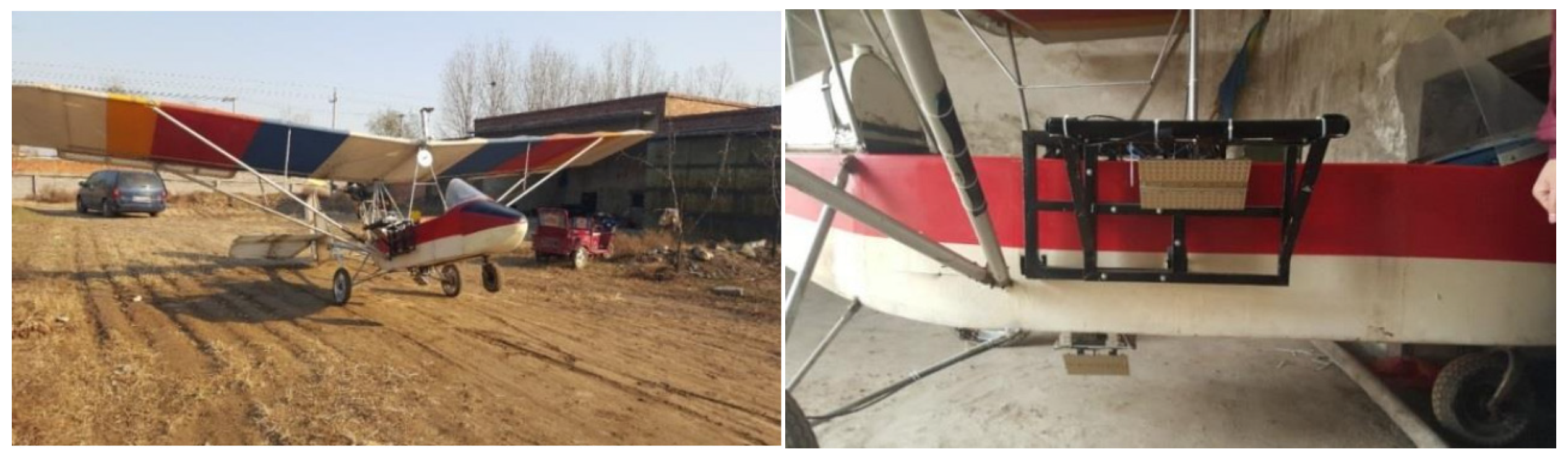
1. Introduction
Radar-based positioning and navigation methods include one-dimensional terrain contour matching [
1,
2] and two-dimensional SAR image matching navigation [
3,
4]. Radar, as an additional sensor, is used to address the drift problem caused by errors in the IMU, especially in situations where GNSS signals are lost or interrupted. The principle of digital terrain matching navigation is that as the aircraft flies over certain specific terrain areas along its flight path, it uses radar altimeters to measure the terrain elevation profile along the path. These real-time measurements are then correlated with pre-stored reference maps to determine the aircraft’s geographical position. Existing terrain matching methods mainly involve correlating altimeter-measured terrain profiles with those in reference maps, which is a line matching approach that lacks resolution in the cross-track direction, leading to potential mismatches, and requiring areas with typical terrain slope characteristics for matching.
Apart from one-dimensional terrain matching, SAR matching navigation achieves a two-dimensional resolution. It matches real-time radar-acquired images with stored SAR images in its database to correct current positional errors. However, SAR scene matching navigation is affected by seasonal changes in terrain features, requiring typical landmarks for reliable matching performance and is challenging to map in areas with significant terrain variations, leading to poor navigation accuracy in mountainous regions. Researchers have focused on two main areas: one is the matching of heterogeneous SAR images, proposing algorithms tailored to SAR image features to improve matching precision and robustness [
5,
6]. The other involves using the positional information of SAR matching points and SAR’s slant range data to establish the relationship between the aircraft and matching points to calculate the aircraft’s position [
3,
7,
8].
InSAR uses interferometry to accurately measure terrain elevation and achieve two-dimensional imaging. It effectively combines the advantages of terrain matching navigation and the SAR image matching navigation methods. InSAR interferometric matching navigation has different working modes. When the terrain undulations in the navigation area are obvious, the InSAR interferometric matching navigation mode is enabled, and the generated interferograms with terrain undulation characteristics are used for matching to achieve platform positioning. When the terrain within the navigation area is relatively flat, single-channel SAR images can be used to complete SAR image matching navigation. Therefore, introducing InSAR technology into positioning and navigation systems offers significant advantages and broad application scenarios. The European Defence Agency (EDA) conducted preliminary analyses of the potential of InSAR-assisted navigation [
9,
10,
11], exploring InSAR parameters and demonstrating the feasibility of InSAR-assisted navigation. They also studied the impact of position and attitude angle errors on phase and positioning errors, as well as the characteristics of digital terrain models. Subsequently, researchers established a platform position inversion model using matched interferogram offsets and proposed using interferometric phase and Doppler frequency to infer the platform’s attitude angles [
12,
13]. Further, a mountain branch point-based InSAR interferometric fringe matching algorithm was proposed to achieve precise matching between interferometric fringes [
14]. Later, researchers began to theoretically analyze high-speed platform positioning based on wrapped InSAR interferograms, providing simulation experiments [
15].
While InSAR demonstrates advantages in accuracy and robustness for matching positioning and navigation compared to traditional SAR, there has not been a complete methodological workflow with real flight data validation for InSAR interferogram matching positioning and navigation so far. Most studies have been based on theoretical analysis and simulations. Therefore, this paper proposes a comprehensive three-dimensional platform positioning method based on InSAR interferogram matching, establishing a robust and high-precision platform positioning and navigation system. The rest of the paper is organized as follows:
Section 2 presents the proposed three-dimensional positioning framework based on InSAR interferogram matching.
Section 3 proposes a method for constructing reference interferograms using external source DEM.
Section 4 proposes a feature matching algorithm suitable for interferometric fringe images, achieving precise matching between actual interferograms and reference interferograms.
Section 5 proposes a three-dimensional positioning model for the platform based on InSAR altimetry geometry.
Section 6 conducts actual InSAR airborne flight experiments, obtaining corresponding positioning results and analyzing positioning accuracy. Finally,
Section 7 presents the conclusions of the paper.
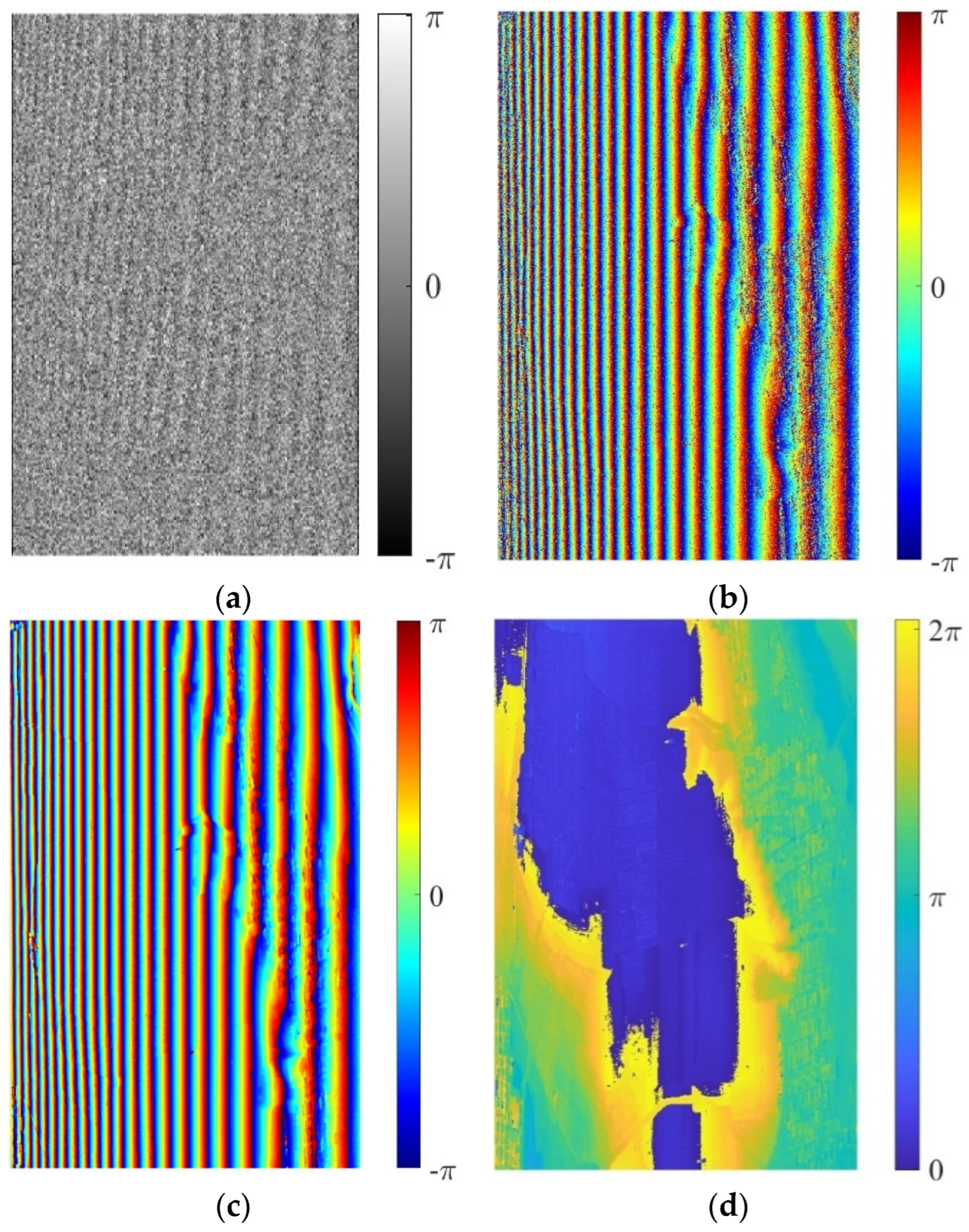
4. Interference Fringe Feature Extraction and Matching
In this section, we need to achieve precise matching between actual interferometric fringes and reference interferometric fringes. In interference fringe matching, due to the influence of drift errors, flight attitude errors, and interference parameter errors, the interference fringe will produce geometric distortion and nonlinear phase errors, so the algorithm based on template matching is not applicable under such conditions. On the other hand, deep learning-based methods are not suitable since there is no relevant interference fringe database. Therefore, we adopt a feature-based image matching algorithm framework.
The classical SIFT algorithm [
19] establishes a linear scale space using Gaussian filters. However, it may not preserve significant phase changes and edge information in the interferometric fringes, affecting the detection of feature points. Instead, we use non-linear diffusion filtering to construct the scale space. When applied to images, non-linear diffusion filtering [
20] represents the brightness of the image through the divergence of the flow function. Non-linear diffusion filtering is expressed by a partial differential equation as follows:
Here,
represents the interferometric phase value,
t is the diffusion time,
div and
are the divergence and gradient operators, and
is the conductivity function. By choosing an appropriate conductivity function, diffusion can be adapted to the local structure of the image. Perona and Malik proposed a way to construct the conductivity function [
21]:
Here,
is the gradient of the interferometric phase
after Gaussian smoothing, and the function
g is defined as:
Here,
K is the contrast factor, controlling the diffusion level. A larger value retains less edge information. By solving the non-linear partial differential equation using the Additive Operator Splitting (AOS) algorithm, we obtain images corresponding to different times in the non-linear scale space:
Here,
I is the identity matrix, and
represents the derivative along the
I direction. After establishing the nonlinear scale space, all pixel points were compared with the surrounding and adjacent pixel points in the two layers above and below. After obtaining feature points, a three-dimensional quadratic function was used for fitting to obtain subpixel positioning results for feature points. The use of nonlinear diffusion filtering to extract feature points in the nonlinear scale space can suppress noise while preserving edge information, thereby increasing the quantity and accuracy of feature points. As shown in
Figure 6, a comparison was made between feature points detected in the linear scale space using the SIFT algorithm and those detected using nonlinear diffusion filtering. It can be observed that the SIFT algorithm detects fewer feature points, and edge points and corners on the fringe map are not sufficiently detected under the smoothing effect of Gaussian linear space. In contrast, the feature points detected using the nonlinear diffusion filter retain edge points and corners, resulting in a higher number of detected feature points.
After determining the positions of feature points, a selection process is applied using the interferometric coherence coefficient to filter out feature points with low coherence. A descriptor is then constructed to form a subset of features. Once key points are selected in the scale space, these key points, being extrema in the scale space, undergo wavelet transformation [
22,
23,
24,
25] to separate multiscale features around the key points, achieving effective feature extraction. Rectangular sub-images are established with key points as centers to describe key point information using sub-region image features, enabling mutual matching between key points in two images. Two layers of 2D discrete wavelet transforms are performed on the sub-region around key points. Since interference fringes contain a significant amount of noise in high-frequency components and texture information in low-frequency components, the first layer’s low-frequency components and the second layer’s low-frequency components are used for feature extraction. Simultaneously, low-frequency components obtained through wavelet decomposition possess translation invariance, enhancing the robustness of fringe matching and making it more resistant to noise, distortions, and other interferences.
After removing the flat ground effect from the interference fringes, which reflects terrain undulation information with a gradually changing gradient, analyzing local gradient information around feature points can effectively describe the current feature points. Histogram of oriented gradient (HOG) is a technique used for texture-based image analysis [
24,
25,
26], simplifying images by extracting gradient information. HOG extracts features that have a locally distinctive shape based on edges or gradient structures. Through block operations, HOG makes local geometric and intensity changes easy to control. If the translation or rotation of an image is much smaller than the scale of local spatial and directional units, the detected differences are minimal. Detecting HOG features in the wavelet domain of two heterogeneous images can effectively describe the texture information around feature points in both images, making it suitable for matching between two images with rich texture features.
First, the low-frequency approximate image extracted through wavelet transformation is divided into blocks. The gradients
in the
and
directions for each pixel in each block are calculated using gradient templates:
For the input image
I, performed convolution operations with the template, respectively, to obtain the gradients
and
in the
x and
y directions:
Thus, we obtained the magnitude
and orientation
of the gradient. Then, we divided
into several ranges, counted the occurrences of gradient directions in different ranges, and formed a histogram of gradient directions. We connected the histograms of gradient directions for each block region to create the HOG feature. This process resulted in a feature vector for each keypoint’s surrounding region in the wavelet domain. The first-level low-frequency components were divided into 4 × 4 cells, and the orientation gradients were calculated for each block region to form a histogram of gradient directions. The second-level low-frequency components were divided into 8 × 8 cells, aiming to increase gradient information around key points and improve matching accuracy.
Figure 7 clearly shows the process of descriptor construction.
Once the descriptor was constructed, the next step involved using the minimum Euclidean distance method for real-time matching of feature vectors between actual and reference interferograms. This process eliminates outlier matches, resulting in pairs of matching points. The three-dimensional position information of the matching points can be obtained by querying latitude, longitude, and height information. The algorithmic flowchart for interferometric fringe feature matching is illustrated in
Figure 8, with the technical process on the left and key step results on the right.
5. Platform Three-Dimensional Positioning Model Based on InSAR Geometry
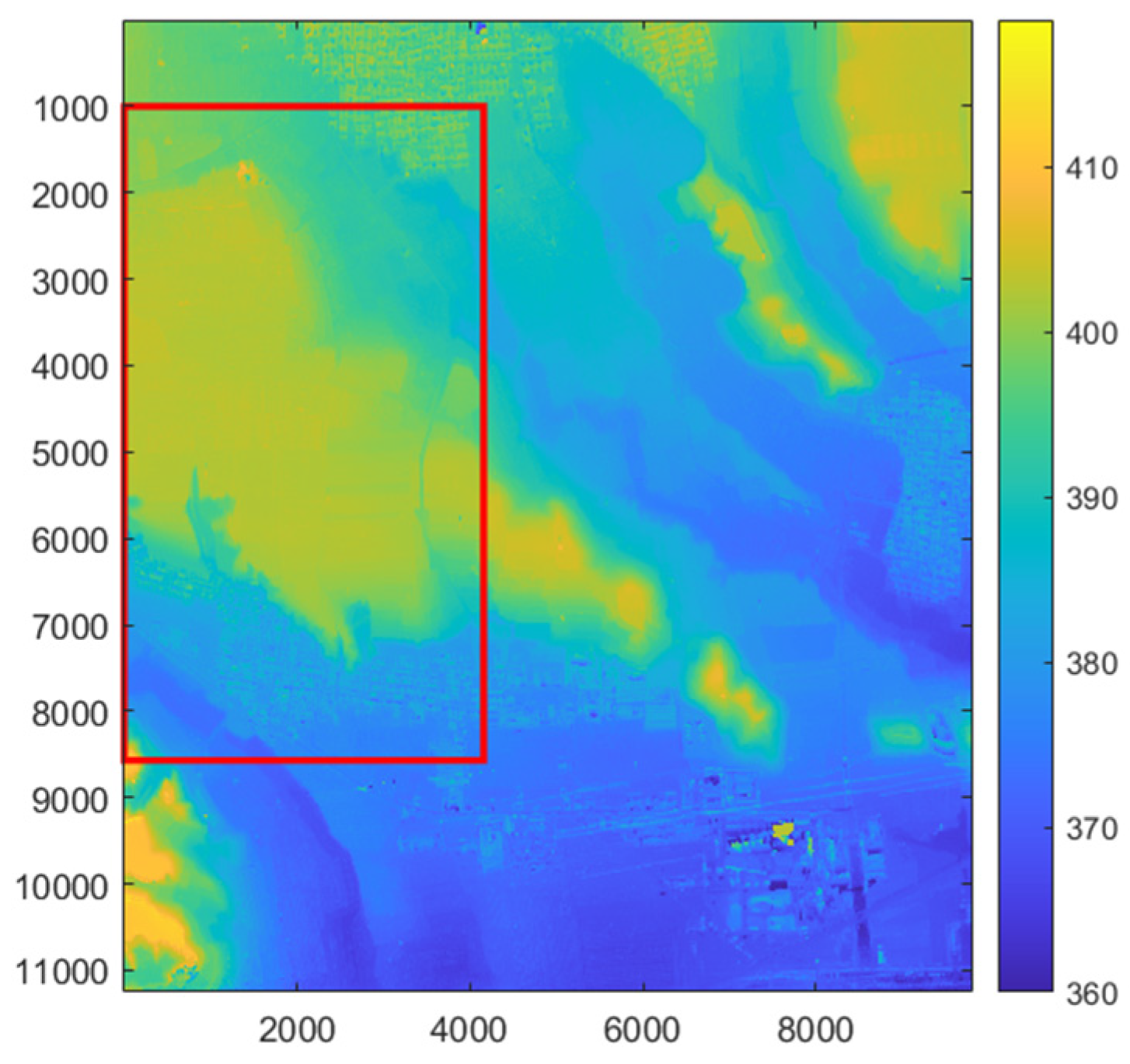
Through the matching of the interferograms, the corresponding position and elevation information for the tie points was obtained, and we established the inversion model of the platform position as shown in
Figure 9. The
x-axis represents the flight direction of the platform, the
z-axis represents the elevation direction, and the
y-axis forms a right-handed coordinate system with the
x-axis and
z-axis.
and
represent the positions of the master and slave radar antennas, respectively,
P represents the matched tie point, and
is the slant range vector from the master antenna to point
P, referred to as the look vector.
is the baseline vector, where
represents the length of the cross-track baseline and
represents the length of the along-track baseline. Orthogonal unit vectors constitute a moving coordinate system, where
is in the flight direction,
is in the same direction as the cross-track baseline, and
is determined using the right-hand rule.
In the moving coordinate system, the unit look vector can be represented as:
where
,
,
, and
represents the inner product operation between vectors. Therefore, the representation of the unit look vector in the moving coordinate system can be calculated as [
27,
28,
29]:
where
is the Doppler centre frequency,
is the platform velocity. The positive or negative sign is determined by the side-looking direction of the radar. The unit look vector is transformed from the moving coordinate system to the carrier coordinate system using the transformation matrix
:
where transformation matrix
is given by:
where
is the angle between the baseline and the
x-y plane. Therefore, the three-dimensional position vector of the platform
can be represented as:
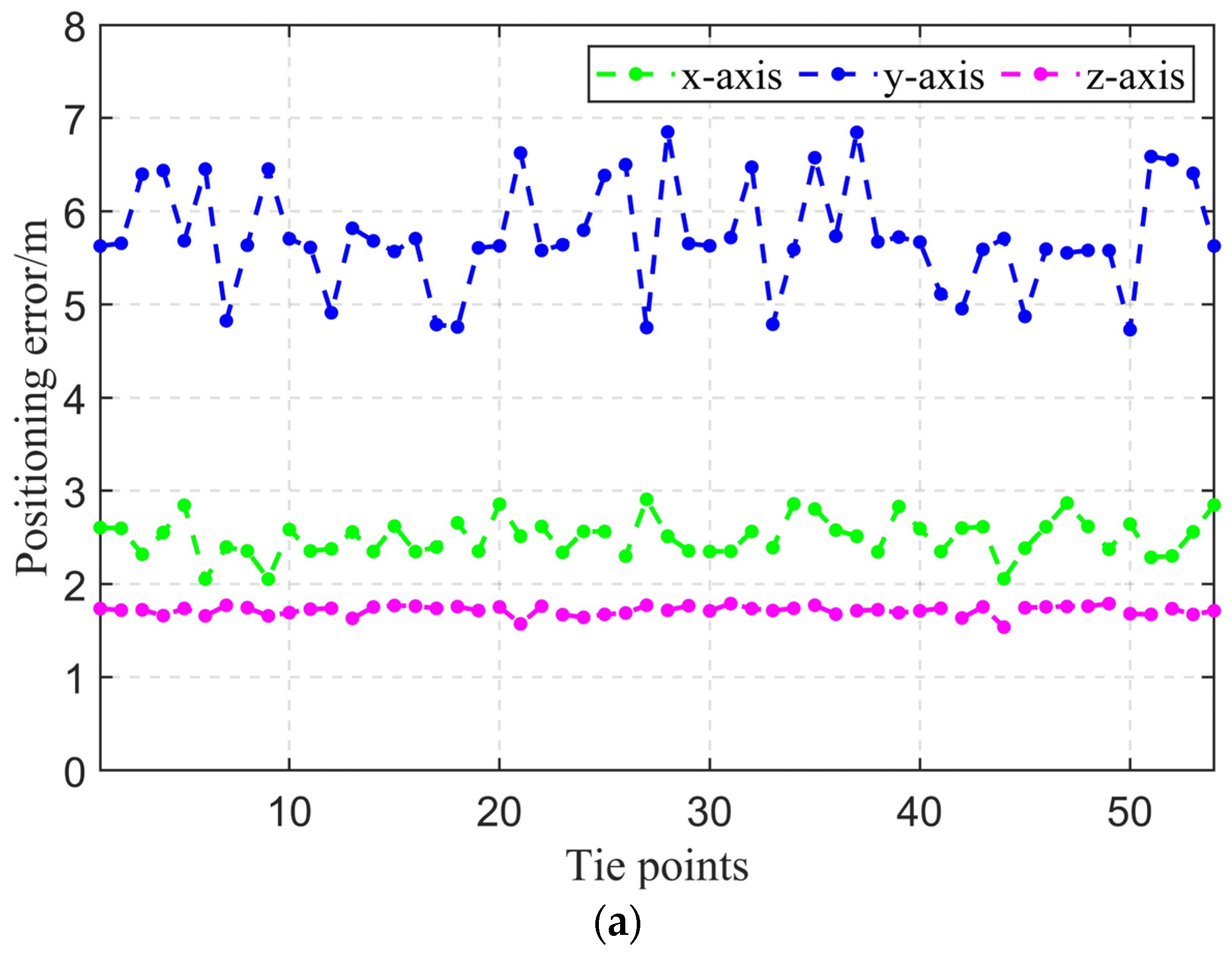
7. Discussion
In this paper, we introduced the application of interferometry techniques to the method of positioning for airborne SAR platforms, utilizing interferograms for matching and positioning. This approach combines the advantages of traditional SAR images and terrain matching positioning methods, leveraging the long-term elevation stability provided by DEMs generated through InSAR mapping, as well as the three-dimensional positioning capabilities of InSAR, thereby improving the final positioning accuracy to be within 10 m. The high precision of InSAR fringe matching is primarily due to the additional information in the elevation dimension provided by InSAR compared to SAR, enhancing the positioning capability from two dimensions to three dimensions. On the other hand, InSAR fringes reflect the undulating nature of the terrain, offering more stability compared to SAR images and thus providing higher stability in the matching process. The error of the results is explained below and some issues are discussed.
7.1. Positioning Error Analysis
The errors in InSAR interference fringe matching navigation mainly include matching errors, platform attitude angle errors, and interference system parameter errors. The interference parameter errors can be eliminated after calibration, so we will not go into details here. Therefore, this section discusses the matching error and platform attitude angle error and their impact on platform positioning, and conducts an error analysis based on the actual parameters of airborne InSAR.
7.1.1. Platform Attitude Angle Error
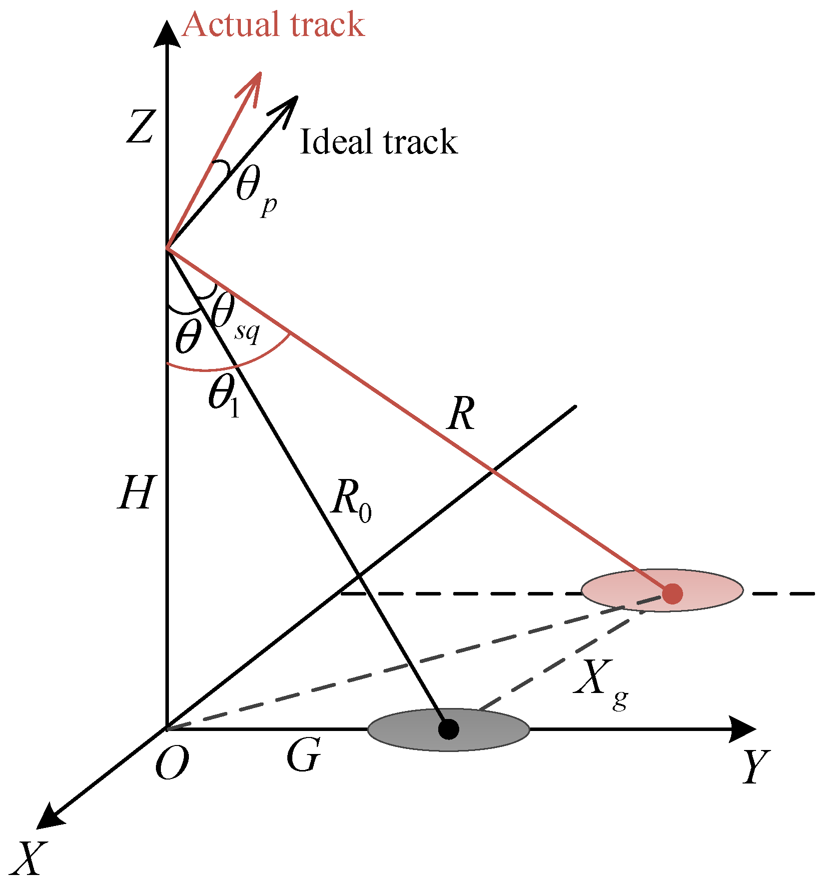
Figure 16 illustrates the positioning error in a plane under the presence of yaw angle error. Since the attitude angle mainly affects the accuracy of plane positioning, an analysis of positional offsets in the azimuthal and range directions is conducted. In the diagram, the aircraft flies along the ideal trajectory. The actual trajectory and the beam illumination area when there is a certain yaw angle error, denoted as
, the actual are indicated in red. The platform flies along the azimuthal direction
x-axis, range direction
y-axis, and vertical direction
z-axis, with
H representing the platform’s flying height. Neglecting terrain fluctuations, the actual slant range matches the ideal trajectory’s slant range, denoted as
. The initial look angle is
, the actual look angle is
, and the slant angle is
. The positioning offset is represented as
.
The slant range
, initial range positioning distance
,
, and
are derived from the geometric relationships in the diagram.
Therefore, the positioning errors in the azimuthal direction
and in the range direction
are:
From the equation, we can determine the influence of yaw angle error on positioning offsets. Using the airborne flight parameters provided in this paper for simulation, with a platform flying height of 1898.86 m and a yaw angle range set to [−0.2, 0.2] degrees, and considering the actual downward viewing angle, which ranges from 30° to 60° from near slant range to far slant range. The results are shown in
Figure 17. It can be observed that the azimuthal positioning error is greatly influenced by yaw angle error, and this influence becomes more pronounced as the downward viewing angle increases. However, the impact on range direction positioning is minimal.
Figure 18 depicts the conceptual illustration of positioning errors in a plane under the presence of pitch angle error. Similar to the analysis method for yaw angle, the aircraft flies along the ideal trajectory. The actual trajectory and the beam illumination area when there is a certain pitch angle error, denoted as
, are depicted in red. The platform flies along the azimuthal direction
x-axis, range direction
y-axis, and vertical direction
z-axis, with H representing the platform’s flying height. Initially, under the ideal conditions, the slant range is denoted as
, while after introducing yaw angle error, it is represented as
. The initial downward viewing angle is
, the actual downward viewing angle is
, and the slant viewing angle is
. The positioning offset is represented as
.
The slant range
, initial range positioning distance
, and
are derived from the geometric relationships depicted in the diagram.
Therefore, the positioning errors in the azimuthal direction, represented by ∆x, and in the range direction, represented by ∆y, are:
From the equation we can determine the influence of pitch angle error on positioning offsets. Using the airborne flight parameters provided in this paper for simulation, with a platform flying height of 1898.86 m and a yaw angle range set to [−0.2, 0.2] degrees, and considering the actual downward viewing angle, which ranges from 30° to 60° from the near slant range to the far slant range. The results are shown in
Figure 19. It can be observed that pitch angle mainly affects azimuthal positioning error and remains relatively constant regardless of changes in the downward viewing angle. The impact on range positioning is minimal.
7.1.2. Fringe Matching Error
Matching errors mainly stem from two aspects: the accuracy of the reference map and the accuracy of the matching algorithm. The spatial resolution and elevation accuracy of the reference map are critical factors determining its quality. A lower spatial resolution implies that each pixel in the image represents a larger actual ground area, which may result in the inability to accurately identify smaller ground features during the matching process, thereby increasing positioning errors. Additionally, if the reference map exhibits geometric distortions, such as shape distortions caused by imaging angles or differences in ground heights, it directly affects the accuracy of positioning. These geometric distortions may cause the matching algorithm to fail to correctly align the reference map with the actual observed image, introducing additional positioning errors. Moreover, inaccuracies in feature point or region extraction during the matching algorithm’s process can also lead to misalignment and matching errors.
According to the geometric positioning model, the matching error transfer relationship in the
x direction,
y direction, and
z direction is:
That is, the matching error and the reference DEM error directly affect the positioning error. Therefore, improving the accuracy of the matching algorithm and using high-precision reference maps can increase the positioning accuracy in equal proportions.
7.2. High-Precision Needs and Future Prospects
The generation of interference fringes is a basic and critical step. It is worth mentioning that in the actual navigation process, the system is a continuous iterative process. After the satellite signal is rejected, the InSAR matching navigation process is started in time, and combined filtering with the INS is performed to obtain the corrected position and attitude information. And imaging, matching, and positioning are continuously performed to reasonably control the interval, accurate position, and attitude information. In addition, even in the absence of precise positioning information to achieve high-precision imaging, image generation and interference processes can be achieved through self-focusing algorithms to obtain interference fringes.
In InSAR matching positioning, the interferometric baseline parameters have a significant impact on the generation of interferograms and the accuracy of three-dimensional positioning, leading to considerable nonlinear distortion in the phase of the reference interferogram and significant errors in the three-dimensional positioning. Therefore, calibration of the interferometric parameters is necessary to ensure high positioning accuracy. Our method involves using matching points on the reference DEM as control points and optimizing the interferometric parameters using the least squares method to ensure the accuracy of these parameters.
Our next step is to optimize the efficiency of the program and adopt parallel processing to meet the needs of real-time operation on airborne platforms, aiming to implement a complete positioning and navigation system.


