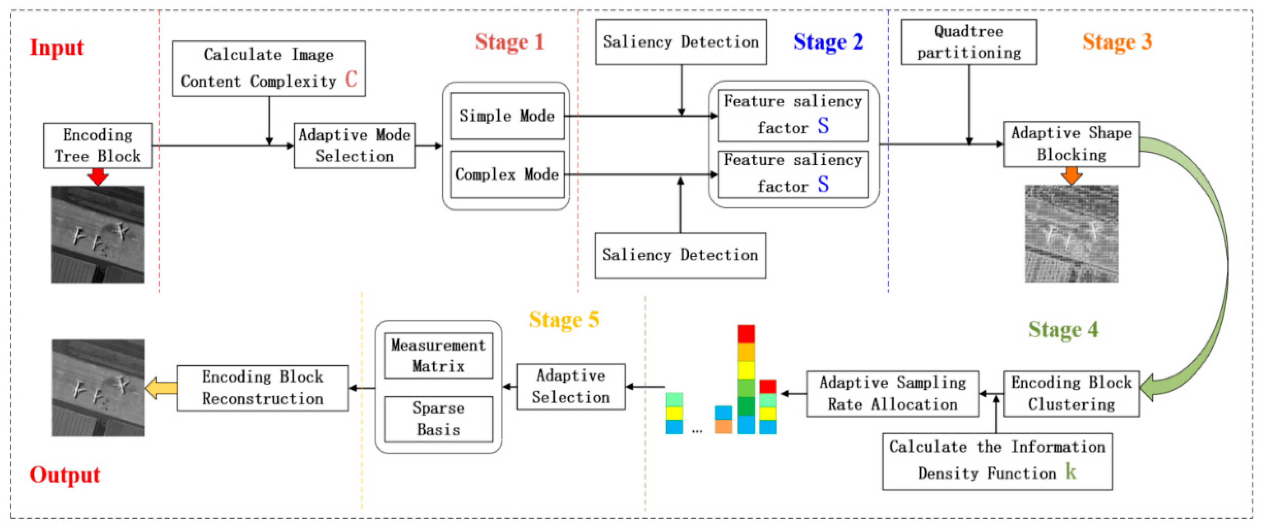
Firstly, this framework uses the maximum between-class variance method to calculate the image content complexity and adaptively selects the coding mode. By extracting image feature factors, a saliency model of the corresponding mode is established to guide the adaptive morphological segmentation of the coding tree block. Then, by using the information density function to detect the sparsity of the encoding block, the sparsity of the image is explored as much as possible to achieve adaptive sampling rate allocation for the image. Finally, the reconstruction matrix and sparse basis are adaptively selected based on the coding block category, and the iteration threshold is set according to the known sparsity. OMP algorithm is used to reconstruct the coding block.
3.1. Adaptive Mode Selection Stage
The image adaptive mode selection stage proposed in this section mainly includes two parts: first, image content analysis, defining the global image complexity calculation function; second, scene model classification, setting threshold parameters for adaptive mode discrimination.
In view of the image content, this article defines an image complexity calculation method based on the maximum between-class variance. According to the grayscale characteristics of the image, the variance is used to calculate the uniformity of the grayscale distribution, and the image is divided into two parts, the foreground and the background. The larger the inter class variance between foreground and background, the greater the difference between the two parts that make up the image, and the more obvious the contrast between foreground and background. And when part of the background is mistakenly classified into the foreground or part of the foreground is mistakenly classified into the background, the difference between the two parts will be reduced, maximizing the inter-class variance means minimizing the probability of misclassification [
22]. Based on the above analysis, by calculating the maximum inter class variance of the encoding tree block, the optimal threshold of the image block is obtained, and the optimal threshold is used for image segmentation. The image complexity
is defined as the number of foreground pixels of the encoding tree block, and the complexity threshold
is set to complete the adaptive mode selection of the encoding tree block.
Based on the maximum between-class variance to evaluate the complexity of image content, the specific mathematical method is as follows: assuming that image pixels can be divided into background and foreground parts according to the threshold, the image with a size of
has a total pixel size of
,
and
are the number of foreground and background pixels, respectively, then the proportion of background and foreground pixels
and
can be expressed as:
If
represents the number of pixels with a grayscale value of
in the background, and
represents the mathematical expectation of the background pixels relative to the entire image, the average grayscale value of the background pixels can be expressed as:
Similarly,
represents the mathematical expectation of foreground pixels relative to the entire image, and the average grayscale value of foreground pixels can be expressed as:
Then the average gray value of the image within the
gray level range is:
The between-class variance is:
Assuming that when the gray level is
, the between-class variance is the largest
, then the image complexity
can be expressed as:
For the scene model, the main purpose of this section is to adaptively select an appropriate processing method based on the image content and maximize the use of the richness of the image to select an appropriate sampling method. According to the global complexity calculation model, the complexity threshold is set as the judgment threshold for the image content complexity . The original image is adaptively divided into two categories: simple and complex. The complex type corresponds to scenery such as cities, forests and clouds, simple types correspond to features such as oceans. In addition, considering the great increase in the resolution of remote sensing images, the image content information represented by a single coding tree block is greatly reduced, and there is a significant disparity between the foreground and background of a single coding tree block (for example: the content of the coding tree block is all ocean), resulting in a bimodal or multimodal between-class variance function, and misjudgment of the maximum between-class variance occurs. Based on this, the optimal threshold constraint is added during mode adaptive selection.
The specific steps of coding tree block adaptive mode selection based on the maximum between-class variance are as follows:
Step 1: Divide each frame/scene of the original remote sensing image into -sized coding tree blocks (CTB).
Step 2: Calculate the histogram of the CTB and normalize it.
Step 3: Set the foreground and background classification thresholds , and iterate from 0.
Step 4: Calculate the between-class variance .
Step 5: , return to step 4 until .
Step 6: Calculate the maximum between-class variance and the optimal threshold .
Step 7: Calculate the image content complexity .
Step 8: Adaptive mode selection, define the adaptive mode selection threshold and the optimal threshold constraint condition . When , it is in simple mode; When and , it is a simple mode; When and , it is a complex pattern.
3.2. Feature Factor Extraction Stage
In addition to conventional statistical features such as variance and information entropy, two-dimensional images also have visual saliency features such as texture and edge information. The edges of an image are the most basic features, and feature maps can be extracted based on the mutation of grayscale, color, and texture structure. The saliency model studied in this section is mainly a pure mathematical calculation method. The purpose of establishing the saliency model is to provide a basis for the adaptive segmentation task of images. The edge detection operator is used to extract the edge roughness information of images, and the corresponding saliency models are constructed for the complex and simple modes in the pattern selection stage. By setting the saliency factor threshold of the global feature map, the quadtree is guided to adaptively partition the image in the next stage.
The edges of images have two attributes: direction and amplitude. Edges can usually be detected through first-order derivatives or second-order derivatives, where the first derivative takes the maximum value as the corresponding edge position, and the second derivative takes the zero crossing point as the corresponding edge position. The research object of this article is that remote sensing images contain noise and radiation stripes. The purpose of the research is to alleviate the resource constraints on the satellite and speed up the processing timeliness. Therefore, noise and processing time are the primary considerations when selecting operators. For this purpose, this section mainly discusses the first-order gradient operator, Sobel operator, Roberts operator, Prewitt operator, Kirsch operator and LoG operator [
23,
24].
Figure 2 shows the edge texture maps of remote sensing images of several typical landmarks such as cities, forests, clouds, and oceans using different operators. It can be observed from the figure that for images with rich content and texture details such as cities, forests, and clouds, the edge details extracted by Sobel operator, Roberts operator, and Prewitt operator are more comprehensive. However, the Sobel operator and Prewitt operator have the phenomenon that the edge is too wide when extracting natural scenes such as forests and clouds, which is not suitable for expressing the saliency of these types of features. For scenes with relatively simple ocean image content, the Sobel operator and Prewitt operator have good performance in extracting sea surface details. Compared to the edge contours of ships, the Prewitt operator is superior. Based on the above analysis, with edge roughness as the salient feature, the Roberts operator and Prewitt operator are used to establish the saliency expressions for complex (such as cities, forests, clouds) and simple (such as oceans) models, respectively.
Based on this, the Roberts operator is used to detect complex CTBs and construct an urban forest pattern saliency model. The correlation between the CTBs and the two Roberts operators can be expressed as:
Among them,
represents the CTB,
, and
are the horizontal and vertical Roberts operators. If the threshold
is set, the local feature saliency factor of complex patterns can be expressed as:
Similarly, use the Prewitt operator to detect simple CTBs and construct a simple pattern saliency model. The correlation
between the CTB and two Prewitt operators can be expressed as:
and
are Prewitt’s two direction operators. If the threshold
is set, the local feature salience factor of the ocean model can be expressed as:
3.4. Sampling Rate Adaptive Allocation Stage
After the CB undergoes two-dimensional discrete cosine transform (DCT), most of the energy is concentrated in the low-frequency part in the upper left corner of the coefficient matrix, while the high-frequency coefficients are distributed in the lower right corner. The expression only contains the cosine term, and the CB can be represented by fewer spectral coefficients. Moreover, when the absolute value of the low-frequency coefficients is greater than the absolute value of the high-frequency coefficients, the CB becomes sparser and the greater the proportion of the low frequency part. In this section. is used as the sparsity judgment threshold of the DCT coefficient . After DCT of the CB, the maximum amplitude coefficient is used to normalize the absolute value of the coefficient. If the normalized coefficient is less than the threshold , the coefficient determined to be smaller is set to 0. Otherwise, the coefficient is regarded as the larger DCT coefficient. represents the number of larger coefficients among the DCT coefficients of each coding block. In this process, the threshold is constant across all encoding blocks, but varies between coding blocks. is used as a measure of sparsity, defined as the information density function of the coding block.
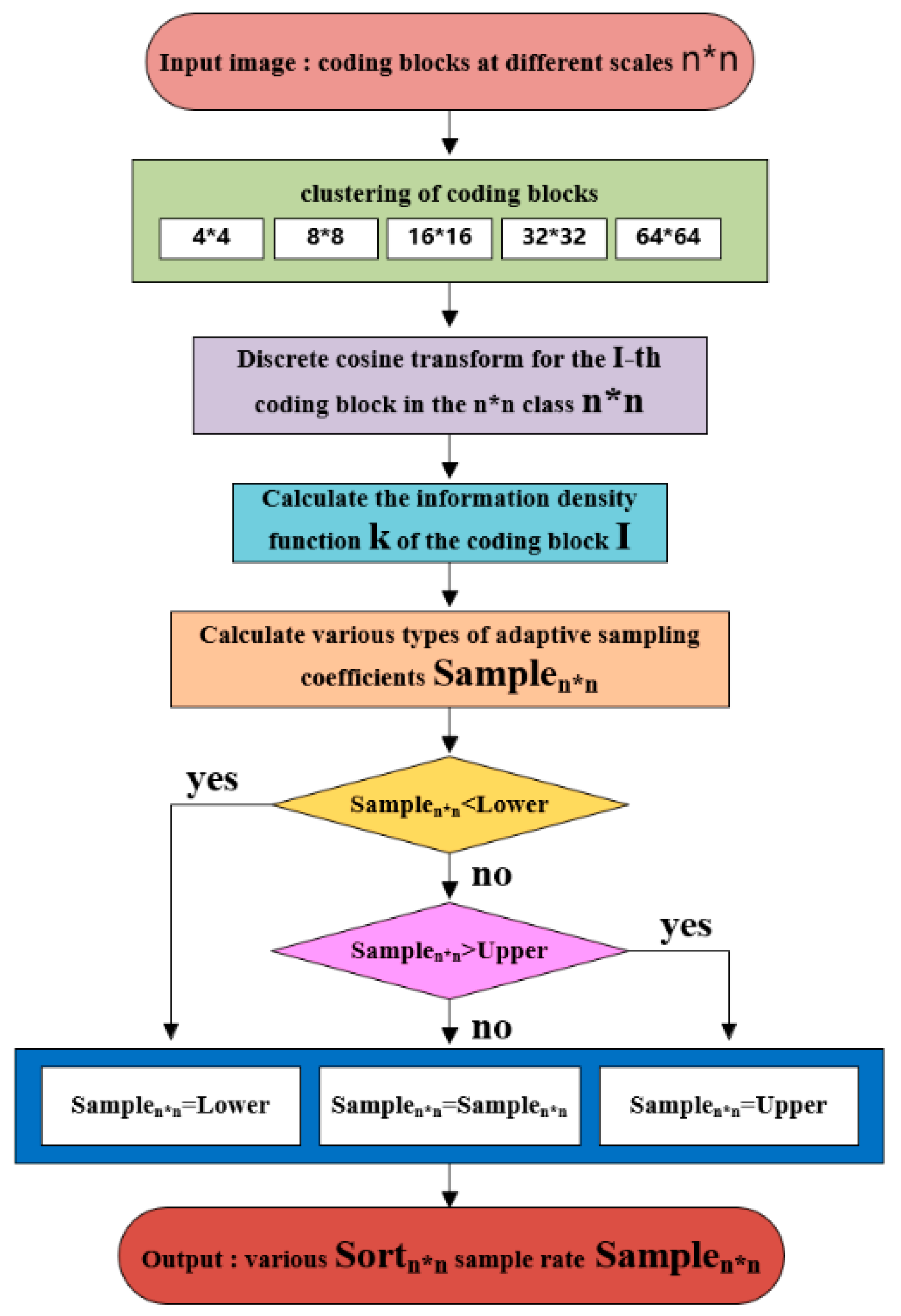
From the above analysis, it can be seen that the smaller the is, the sparser the coding block is, and the better image reconstruction can be achieved through fewer sampling points. This section adaptively allocates the sampling rate to the image block by calculating the information density function of the CT. However, in the actual image processing process, an image may contain many -sized CTBs, and a CTB can be adaptively divided into multiple CBs of different sizes, especially high-resolution and large-width remote sensing images. Assigning a sampling rate to each CB undoubtedly increases the burden of on-board storage and transmission. Based on this, this article adopts clustering method to cluster CBs with the same size in an image into one category, and assign the same sampling rate to the CBs in the category according to their average information density. In fact, for large-scale images, there may be hundreds to thousands of CBs in a class. Considering the compression timeliness issue, if the number of CBs in the category is less than 10, the average information density of all blocks is calculated; while if it is greater than 10, 10 CBs are randomly selected to calculate the average information density.
Furthermore, according to the principle of compressed sensing, image reconstruction relies on both the measurement results and the prior of signal sparsity. Therefore, the number of measurements
depends largely on the sparsity
of the CB, rather than the length
of the CB. For high-quality reconstruction of the CB, the following constraints must be satisfied [
25]:
where
is a constant. In practical situations, according to the rule of thumb, the number of measured values
must be at least three times greater than the sparsity
.
Figure 3 is a flow chart of the sampling rate adaptive allocation method based on information density function and the specific algorithm is shown in Algorithm 2.
| Algorithm 2. Sampling rate adaptive allocation algorithm based on information density function. |
| Task: Adaptive allocation of sample rate to different scale CBs |
|
| Step: |
| according to the size. |
| , randomly select 10 CBs to calculate the DCT coefficients. |
| (3) Calculate the CB information density function : |
|
| : |
|
| : |
|
|
3.5. Image Adaptive Reconstruction Stage
Most traditional compressed sensing reconstruction algorithms use a fixed observation matrix for the observation samples of all CBs, such as Gaussian random matrix, Bernoulli random matrix, partial Fourier matrix, Toeplitz matrix, Hadamard matrix, etc. This naturally ignores the image content and texture structure, does not fully exploit the sparsity of the image, and the sparsity is different between different CBs. Applying the same sampling rate can easily cause the reconstructed image to be highly pixelated.
Based on the image adaptive coding in
Section 3.1,
Section 3.2,
Section 3.3 and
Section 3.4, this section proposes an adaptive block compressed sensing-orthogonal matching pursuit algorithm (ABCS-OMP) in the decoding and reconstruction stage. The reconstruction matrix and sparse basis are adaptively selected for the CB category, the iteration threshold is set according to the known sparsity, and the OMP algorithm is used to reconstruct the image block.
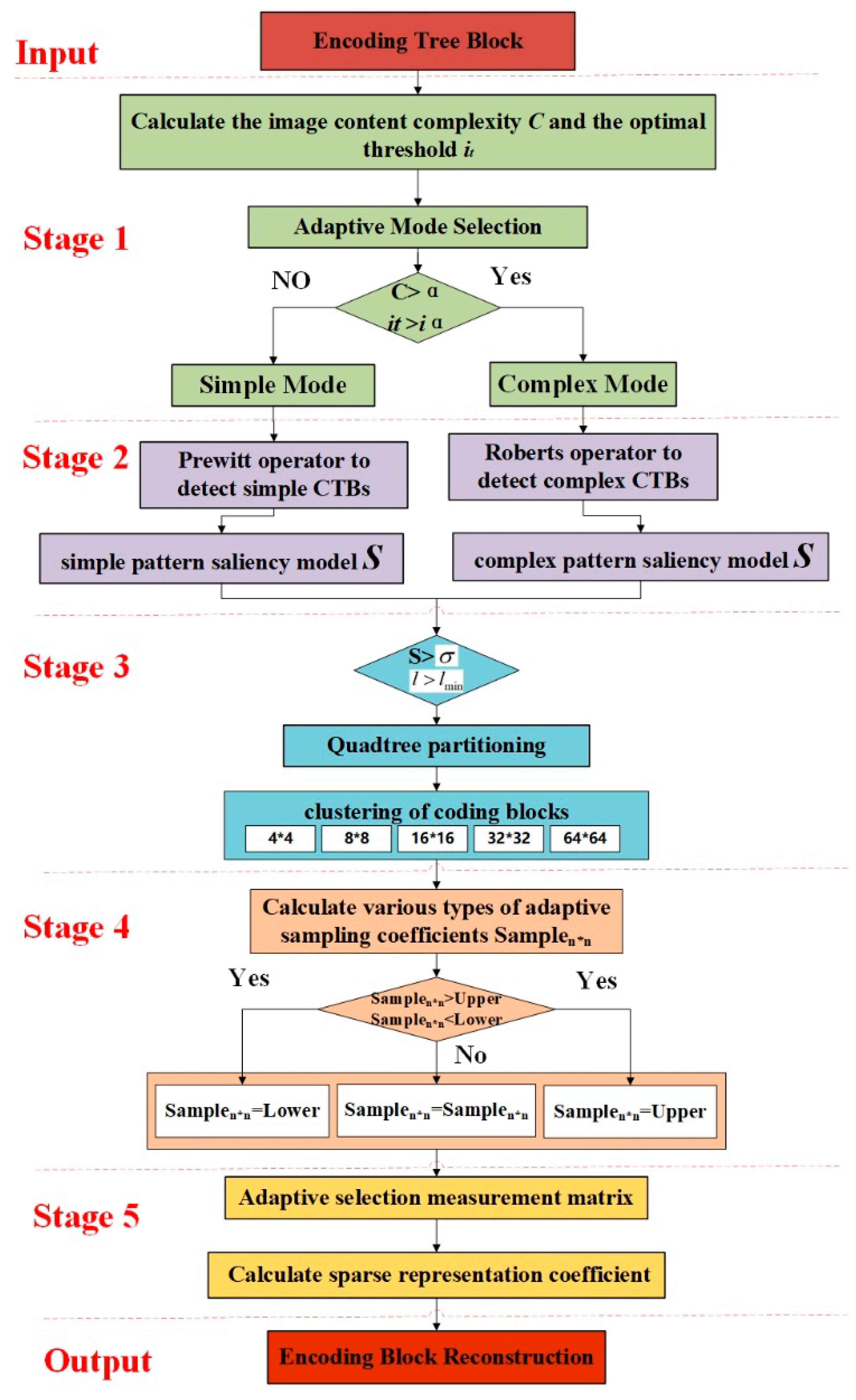
Figure 4 is the complete workflow structure diagram of the remote sensing image fully adaptive coding and decoding compressed sensing framework designed in this paper, in which the ABCS-OMP algorithm is shown in Algorithm 3, where the input in Algorithm 3 is the measured value of the image after adaptive sampling and observation, and the output is the adaptive reconstruction algorithm to restore the measured value to the original image.
| Algorithm 3. Adaptive decoding-orthogonal matching pursuit algorithm based on CS. |
| Task: Coding block adaptive decoding reconstruction |
| Input: observation value |
| Step: |
| . |
| : |
|
| . |
| . |
| . |
| and return to Step 3. |
| : |
|

 ,
, 


