Article

Combining LiDAR and Spaceborne Multispectral Data for Mapping Successional Forest Stages in Subtropical Forests

by
Bill Herbert Ziegelmaier Neto
1,
Marcos Benedito Schimalski
1,*,
Veraldo Liesenberg
1,
Camile Sothe
2,
Rorai Pereira Martins-Neto
3 and
Mireli Moura Pitz Floriani
4
1
Departament of Forestry Engineering, Center of Agroveterinary Sciences, Santa Catarina State University, Lages 89500000, SC, Brazil
2
Planet Labs PBC, San Francisco, CA 94107, USA
3
Faculty of Forestry and Wood Sciences, Czech University of Life Sciences Prague, Kamycka 129, 16500 Prague, Czech Republic
4
Klabin Corporation, São Paulo 04538132, SP, Brazil
*
Author to whom correspondence should be addressed.
Submission received: 6 February 2024 / Revised: 10 April 2024 / Accepted: 18 April 2024 / Published: 25 April 2024
(This article belongs to the Special Issue Lidar for Forest Parameters Retrieval)

Abstract

:
The Brazilian Atlantic Rainforest presents great diversity of flora and stand structures, making it difficult for traditional forest inventories to collect reliable and recurrent information to classify forest succession stages. In recent years, remote sensing data have been explored to save time and effort in classifying successional forest stages. However, there is a need to understand if any of these sensors stand out for this purpose. Here, we evaluate the use of multispectral satellite data from four different platforms (CBERS-4A, Landsat-8/OLI, PlanetScope, and Sentinel-2) and airborne light detection and ranging (LiDAR) to classify three forest succession stages in a subtropical ombrophilous mixed forest located in southern Brazil. Different features extracted from multispectral and LiDAR data, such as spectral bands, vegetation indices, texture features, and the canopy height model (CHM) and LiDAR intensity, were explored using two conventional machine learning methods such as random trees (RT) and support vector machine (SVM). The statistically based maximum likelihood (MLC) algorithm was also compared. The classification accuracy was evaluated by generating a confusion matrix and calculating the kappa index and standard deviation based on field measurements and unmanned aerial vehicle (UAV) data. Our results show that the kappa index ranged from 0.48 to 0.95, depending on the chosen dataset and method. The best result was obtained using the SVM algorithm associated with spectral bands, CHM, LiDAR intensity, and vegetation indices, regardless of the sensor. Datasets with Landsat-8 or Sentinel-2 information performed better results than other optical sensors, which may be due to the higher intraclass variability and less spectral bands in CBERS-4A and PlanetScope data. We found that the height information derived from airborne LiDAR and its intensity combined with the multispectral data increased the classification accuracy. However, the results were also satisfactory when using only multispectral data. These results highlight the potential of using freely available satellite information and open-source software to optimize forest inventories and monitoring, enabling a better understanding of forest structure and potentially supporting forest management initiatives and environmental licensing programs.

1. Introduction

Traditional forest inventories in tropical forests require time and resources, which adds to the difficulty of accessing certain areas to collect information. The costs associated with field surveys are usually high, which is why they are usually conducted at irregular intervals [1]. This makes it difficult to track forest dynamics and successional stages, hampering the implementation of management and conservation strategies, which can have serious consequences for threatened tropical biomes such as the Atlantic Rainforest. This biome has been reduced to 28% of its original area [2] due to anthropogenic disturbances such as industrial activities, urbanization, and agricultural expansion. Currently, the Atlantic Rainforest consists of forest patches at different stages of forest succession embedded in a mosaic of degraded areas, pastures, agriculture, forestry, and urban areas [3].
The classification of the forest succession process into different stages is a strategy for understanding forest dynamics and characteristics [4]. For Brazilian legislation, the modalities of use and standards for vegetation suppression in the Atlantic Rainforest biome are regulated differently for each successional stage, making it important to classify them not only accurately but also in a timely manner for environmental enforcement and permitting [5]. Measurements of structural attributes related to forest succession are also important for predicting long-term processes such as carbon sequestration [6]. Identifying and understanding the ecological relationships within different successional stages is fundamental for maintaining existing ecological values and identifying strategies for restoring degraded areas [7].
Because classification of different successional stages on a large scale and in a continuous manner is not feasible using traditional field surveys, there is a need to investigate data and methods that map forest succession more efficiently and rapidly to optimize traditional field inventory techniques [7,8]. One alternative is the use of airborne LiDAR (Light Detection and Ranging) technology, which transmits and receives a laser pulse. LiDAR produces three-dimensional information from the forest canopy and the ground, providing accurate estimates of structural attributes [9,10]. Parameters such as tree height and canopy dimensions are important elements for management [11]. LiDAR metrics characterize the distribution and density of vegetation, which vary with the successional stage, making it possible to classify the forest successional stages over large areas [12,13].
The sensitivity of certain types of remote sensing data, such as LiDAR and SAR, to measure the three-dimensional structure of the vegetation canopy enhances their ability to provide accurate estimates of vegetation structure, since succession is a three-dimensional process [7,14,15]. Many studies have demonstrated the importance of remotely sensed data from LiDAR or optical sensors for a variety of land applications. Some studies have used airborne LiDAR for biomass estimation in temperate forests [16,17], or for ecological surveys and carbon stock assessment in tropical forests [18,19]. Some studies have used metrics provided by LiDAR data to classify successional stages [19,20,21,22]. Other authors have used optical data for land use, land cover, and vegetation classification [23,24,25,26,27]. Despite the ability of airborne LiDAR data to represent the vertical structure of vegetation and the terrain in which it is located, its cost can still be considered high, especially in developing countries [7].
Alternatively, many optical sensors on board satellites provide free and global information. They are used for a variety of purposes, including natural resource exploration and thematic mapping, environmental monitoring, natural disaster detection, crop forecasting, defense, and surveillance. Many of these applications are only possible because of the improvement in the ability of imaging sensors to produce more accurate information, with some sensors having spectral resolution of hundreds of bands and spatial resolution better than 1 m [28,29]. In recent years, several Earth-observation satellites have been launched, providing data with steadily improving spectral, radiometric, and spatial resolutions [27]. Among them, Landsat-8 and -9 and Sentinel-2 have been explored in many forest applications, such as aboveground biomass estimation [30], burn severity mapping [31], and even forest succession stage classification [27]. Other potential optical sensors have been introduced but have not been as well studied for these applications. Among them, CBERS-4A was launched on 20 December 2019, which has three sensors: a multispectral camera (MUX), wide field imaging camera (WFI), and wide scan multispectral and panchromatic camera (WPM). This WPM sensor has a high spatial resolution of 2 m in the panchromatic band, a radiometric resolution of 10 bits, and a spectral resolution of 4 bands. Another sensor is the PlanetScope, which has a radiometric resolution of 16 bits and a spatial resolution of 3 m. It currently has eight spectral resolution bands and offers the possibility of daily temporal resolution. Given that all these sensors provide data with different spatial, spectral, and temporal resolutions, there is a need to understand whether any of these four sensors stand out for the classification of successional forest stages, with the advantages and disadvantages of each.
Compared to spaceborne multispectral data, airborne LiDAR data are typically available at smaller scales. Nevertheless, studies have shown the potential of using data from both airborne LiDAR and satellite-based imaging sensors for forest successional stage classification [32,33]. However, to our knowledge, no study has compared the performance of multispectral sensors from these four satellites (CBERS-4A, PlanetScope, Sentinel-2, and Landsat-8) in conjunction with LiDAR data for this purpose. Due to the availability of a variety of open and commercial multispectral satellite data, it is important to be aware of and understand the strengths and weaknesses of each for forest classification. This allows users to make better decisions when implementing conservation and management strategies while conserving resources.
In addition to the selection of the most appropriate data, the chosen classification method is also critical for successful land cover and land use mapping [34]. The use of multispectral spaceborne data combined with large-scale automatic classification techniques reduces the inconsistencies associated with human interpretation [35,36]. In this context, traditional statistical and machine learning algorithms are widely used due to their ability to handle high-dimensional data with a limited number of samples [37]. They are easier to interpret compared to advanced deep learning algorithms [38]. In machine learning (ML), nonparametric algorithms are used for area modeling and classification. These algorithms accept a variety of data as input predictor variables and refrain from making assumptions about them [39,40]. Random Tree (RT) and Support Vector Machine (SVM) are examples of this type of algorithm. On the other hand, parametric algorithms assume that the regression function can be parameterized with a finite number of parameters [41]. Statistical and probabilistic models assume that the input data are described using a Gaussian distribution and allow statistical inference to describe these distributions [42,43,44], such as the maximum likelihood classifier (MLC).
This study proposes a method for classifying forest successional stages in a subtropical forest area in southern Brazil, combining LiDAR and multispectral data from four platforms: CBERS-4A, PlanetScope/Dove, Sentinel-2, and Landsat-8, two of which have never been used for this purpose. The canopy height model (CHM) was extracted from the LiDAR data, validated with field data, and used as an attribute in some classification approaches. From the four multispectral sensors, additional texture-related metrics were extracted, and the addition of some vegetation indices was also considered. In addition to testing datasets composed of different attributes and sensors, different classification methods were compared: a traditional parametric classification method, MLC, and two machine learning methods, RT and SVM. The accuracy of the classifications was evaluated using conventional forest inventory data and manual photo interpretation of CBERS-4A data and an unmanned aerial vehicle (UAV) mosaic. The results of this study help to understand how sensors with different capabilities influence classification accuracy in discriminating forest succession stages in an Atlantic rainforest, and such information can help decision makers implement conservation and management strategies in this threatened biome.

2. Materials and Methods
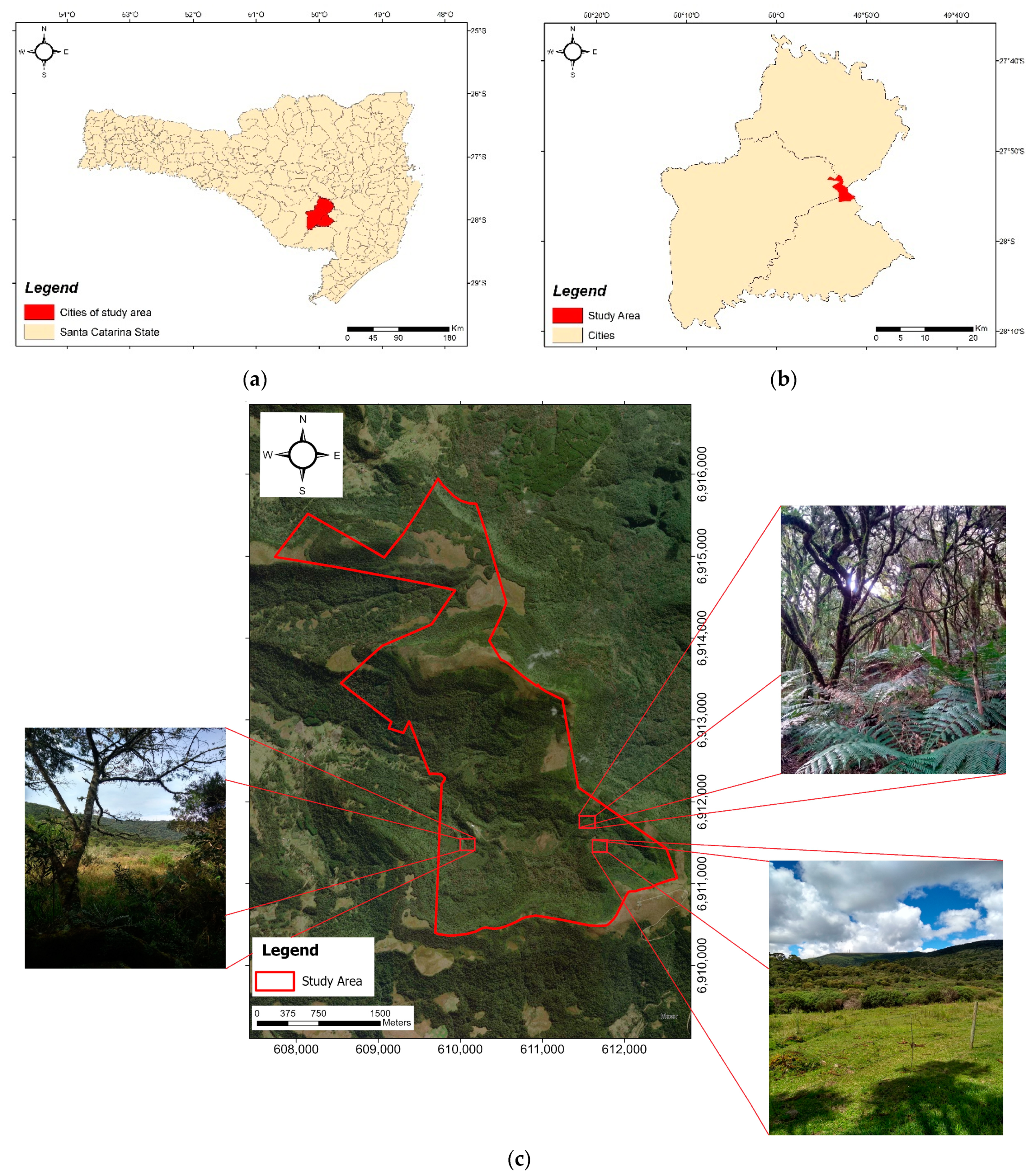
2.1. Study Area

The study area is a Private Natural Heritage Reserve (https://klabin.com.br/sustentabilidade/meio-ambiente-e-biodiversidade/rppns, accessed on 17 April 2024) and is located in the municipalities of Bocaina do Sul, Painel, and Urupema (Santa Catarina state; Southern Brazil; Figure 1). This region has a Cfb climate (humid mesothermal temperate climate with mild summers) [45]. The predominant vegetation in the region is classified as Upper Montane Mixed Ombrophyllous Forest [46], with an average elevation of 1525 m above sea level, and it belongs to the Atlantic Forest biome. According to forest inventory data provided by the organisation, the predominant species in the area are Araucaria angustifolia, Dicksonia sellowiana, Drimys angustifolia, Drimys brasiliensis, Eugenia pyriformis, Ilex microdonta, Ilex paraguariensis, Myrcia palustris, and Siphoneugena reitzii. Figure 1 shows the map of the study site containing the property’s boundaries.

2.2. Data Collection and Processing

Six data sources were selected for this study: an LiDAR point cloud, multispectral spaceborne imagery from CBERS-4A, Landsat-8, Sentinel-2, and PlanetScope, and a mosaic obtained from a UAV flight. Figure 2 shows the point cloud information and processing steps distributed in the processing flowchart. The detailed procedures of each processing step are described in the following sections.

2.2.1. LiDAR Data

Table 1 shows the sensor and settings used for the LiDAR data acquisition. The aerial survey was performed by SAI—Serviços Aéreos Industriais—October 2019. The CHM was generated by filtering and classifying the LiDAR point cloud using the method developed in previous studies [47,48] in Lastools v.2020.

2.2.2. Description of the Multispectral Satellite Data

The data from CBERS-4A (WPM sensor) and PlanetScope are from 17 April 17 2020. The scenes used were “CBERS_4A_WPM_20200312_206_146_L4” and “20201704_142122_94_1069_3B_AnalyticMS_SR”, respectively. The Landsat-8/OLI data are from March 10, 2020, corresponding to the scene “LC08_L1TP_221079_20200310_20200822_02_T1”, and from Sentinel-2/MSI, we used a scene from 24 April 2020, “L2A_T22JFQ_A016366_20200424T132408”.
The CBERS-4A images have been downloaded from the INPE website (http://www.dgi.inpe.br/catalogo/explore, accessed on 17 April 2024), and have three sensors: multispectral camera (MUX); wide field imaging camera (WFI); and wide scan multispectral and panchromatic camera (WPM). The WPM sensor provides 2 m spatial resolution in the panchromatic band, 10-bit radiometric resolution, and four spectral bands from visible to near-infrared. Images from the Landsat-8/OLI platform are available on the USGS website (https://earthexplorer.usgs.gov/, accessed on 17 April 2024) and have a spatial resolution of 15–30 m and a 16-bit radiometric resolution.
Sentinel-2 data are available on the Copernicus website (https://dataspace.copernicus.eu, accessed on 17 April 2024). This platform consists of a pair of imaging satellites and has a spatial resolution of (10–60 m), 12-bit radiometric resolution, and high spectral resolution with 13 bands. The three platforms mentioned above make their data freely available.
On the other hand, PlanetScope images are commercially available through the Planet website (https://www.planet.com/, accessed on 17 April 2024). This platform has a constellation of satellites with 16-bit radiometric resolution, 3 m spatial resolution, and currently four spectral bands, in addition to high temporal resolution. The free images with the data closest to the LiDAR coverage were used. Since there is a time lag between the data acquisition dates, there may be differences in vegetation characteristics between them. Table 2 shows the bands used along with the spectral resolution of each image.

2.2.3. Preprocessing Satellite Images

The CBERS-4A, Planet, and Sentinel-2 satellite data already have atmospheric and geometric corrections. For the Landsat-8 images, the semi-automatic classification plugin [49] in the QGIS 3.22 application was used. The preprocessing tool was used to perform atmospheric correction based on the .MTL files provided with the images. Geometric corrections were also applied to these images.
After the atmospheric correction, the images were subjected to a band composition to obtain color images, which were then used to extract texture metrics. For the images with the panchromatic band, the sharpness weight of the bands was calculated, considering the radiance within each band [50]. Then, to increase the spatial resolution of the Landsat-8 and CBERS-4A images, the pan sharpening between the color compositions and the panchromatic band was performed using the weight value of each of the previously calculated bands and the Gram–Schmidt method, which is based on a vector orthogonalization algorithm [51].
Finally, using the raster calculator tool, the following vegetation indices presented in Table 3 were generated for all satellites through mathematical operations between the bands.
The multispectral images were converted into a gray level image by applying weights for each band and normalizing the output image using the gray level function [57]. Then, the gray level image was used to extract the texture information. Using the Haralick method [58] empirically and considering the pixel size of the images, and with the search window (3 × 3, 5 × 5, and 7 × 7), the azimuth value of 135° [24] was extracted. As a result, information on energy, entropy, correlation, contrast, and homogeneity of variance was extracted. This process was performed for all satellite images examined. At the end of the preprocessing steps, all data were resampled to 1 m spatial resolution to allow integration with LiDAR-derived data. This resampling of multispectral data to 1 m did not change the spectral and spatial characteristics of these datasets, as each 15 m or 10 m pixel size (depending on the multispectral sensor) is divided into a 1 m pixel size that reflects the same information as its original resolution. This procedure is only intended to make the multispectral data compatible with the LiDAR spatial resolution, while not degrading the resolution of the LiDAR data. We are aware that some polygons used as training samples may contain only partial information of the original pixel size. However, since our targets are natural forests and not individual objects such as trees, we felt that this effect would not be as pronounced.

2.2.4. Reference Classification

The elaboration of the reference classification, or ground truth, was carried out using information from the conventional forest inventory provided by the company that owns the area where the study was conducted, the CHM (Appendix A, Figure A1), and manual photointerpretation using the CBERS-4A satellite image, which has the best spatial resolution among the images used. The mosaics generated using the UAV were used to validate the photointerpretation, since flights were only performed in some parts of the study area, and these did not provide enough information to generate the reference classification. The forest height provided by the CHM was the main information used for class delimitation, together with the visual analysis of the CBERS-4A image.

2.2.5. Unmanned Aerial Vehicle (UAV)

To evaluate the reference classification, images with very high resolution were acquired from UAV Parrot Blue Grass. Table 4 shows some characteristics of the platform.
The flight altitude was 120 m, with a longitudinal and lateral overlap of 80% and a flight speed of 5 m/s. The resulting pixel size information was 11.31 cm/pixel, with an approximate flight time of 13 min based on the established parameters. Six areas of approximately 16 hectares each were selected for the aerial survey.
After the UAV data collection, they were subjected to automatic aerial triangulation and digital orthomosaic creation using the WebODM 2.4.2 software. The high-resolution processing parameter was used to obtain the photogrammetric point cloud of the area of interest, leaving its options as default. The UAV mosaics were used to validate the manual photointerpretation generated from the CBERS-4A image and the data derived from LiDAR. The UAV campaign was conducted in April 2021, with a time lag between the LiDAR campaign and the natural forest areas, which are well established and have not suffered the effects of anthropization.

2.2.6. Datasets Creation

For each satellite used (CBERS-4A, Sentinel-2, Landsat-8, and Planet), 11 datasets were created to use all the available information (spectral bands, vegetation index, GLCM, and LiDAR information) for that satellite or sensor. All data combinations were obtained for each satellite, and data from different satellites were not combined. Table 5 shows the input data settings used in the classification process.

2.3. Image Classification

Training and validation polygons were created to provide the classification algorithms with information about the classes of interest to perform image classification. Since all data were resampled to 1 m spatial resolution, the same samples were used for different datasets.
For the classification in this study, a pixel-oriented classification approach was also used. Despite the advent of high and ultra-high spatial resolution digital images, object-based classification has been developed [59,60]. Object-based classification differs from pixel-based classification in two ways. The first is that object-based classification is performed on object units derived from the image segmentation process, whereas pixel-based classification analyzes image pixels directly. The second is that pixel-based classification uses their spectral properties. At the same time, object-based classification uses not only the spectral properties but also the spatial, textural, and shape properties of objects [59,60]. Despite these differences, both techniques have achieved relatively satisfactory performance in extracting land cover information from various remotely sensed images [59,60], each with its advantages and limitations. Pixel-based classification does not alter the spectral properties of pixels and can preserve these properties [60]. Although object-based classification can exploit the spectral and complementary properties of objects, the spectral properties of objects are smoothed by image segmentation [61]; segmentation errors caused by under-segmentation and over-segmentation can affect the accuracy of object-based classification results [62]. Over-segmentation occurs when a semantic object is divided into several smaller image objects, while under-segmentation occurs when different semantic objects are grouped into one large image object. From a classification perspective, over-segmentation and under-segmentation have different effects on the potential accuracy of object-based classification [62]. For over-segmentation, each object corresponds to a class, so it is possible to classify all pixels in an over-segmented image object to their true class. However, for under-segmentation, it is impossible to classify image objects into their true classes because each under-segmented image object overlaps with multiple classes, but the image object is classified into only a single class [62]. Due to the characteristics of the natural forest canopy, with its high variability of species and canopy sizes, it is possible to introduce a classification error due to the segmentation used, for example by grouping different successional classes together. For this reason, pixel-based classification was chosen for this study.

2.3.1. Sampling

To create the samples, polygons for the different classes of the area were generated using the Region of Interest (ROI) tool of the Arcmap 10.4 software, based on field inspections and photo interpretation. These data were then randomly divided into training (±70%) and validation (±30%) samples. The classes sampled were “field”, “water”, initial successional stage “SS1”, intermediate successional stage “SS2”, and advanced successional stage “SS3”. Table 6 shows the areas obtained from the reference classification of each class in hectares (ha), and Table 7 shows the number of pixels sampled per class. The same calibration and validation samples were used for all models. Appendix A Figure A2 shows the spatial distribution of the samples over the study area.

2.3.2. Supervised Classification

Three classification algorithms were used to classify the datasets: RT, SVM, and MLC, using the tools available in Arcmap 10.4. First, empirical tests were performed to define the parameters of each classifier to train the classification algorithm. For the RT, the maximum-number-of-trees parameter was set to 50, the maximum tree depth was set to 30, and the maximum number of samples per class was set to 1000. For the SVM algorithm, the maximum number of samples per class was set to 500, and Arcmap does not indicate which kernel the tool is using. The MLC used only the variance and covariance of the class signature to assign each pixel to one of the classes [63].
The classifiers mentioned above adjusted a classification model based on the training samples performed for each of the datasets of the four satellites. The classified image was generated based on the classification of the respective dataset using the model trained in the previous step. The confusion matrix [64] was generated from the evaluation points created within the validation polygons. These points extracted the class information from the classified image and the reference classification to construct the matrix by comparing these two data.

2.4. Accuracy Assessment

All the accuracy assessment measures were created from validation samples (±30%). The confusion matrix allowed the calculation of the overall accuracy, weighted kappa index [65], standard deviation of the kappa index, and its minimum and maximum values. In addition, the producer’s and user’s accuracy was calculated. It was also verified whether there was a statistical difference between the mean height values of the inventory and the CHM, using Student’s t-test, and between the kappa values, using the Z-test [66], both tests having 95% significance.

3. Results

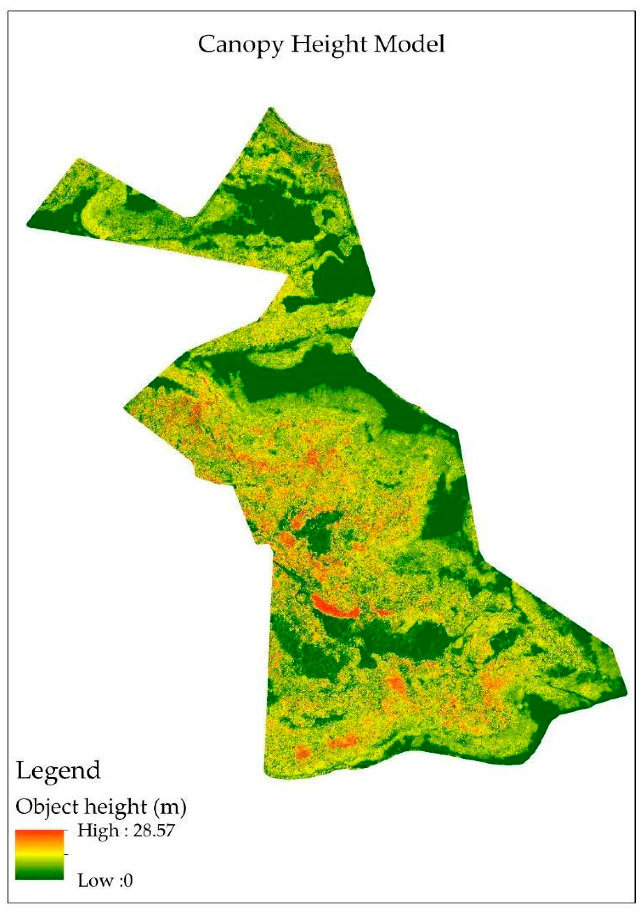
3.1. Canopy Height Model

One of the steps in this study was to generate the CHM to be used as an attribute in the successional stage classification. The CHM was generated by classifying and filtering the LiDAR point cloud (Figure 3) and subtracting the resulting Digital Terrain Model from the Digital Surface Model [48]. This product provided information on the vertical structure of the vegetation as an alternative to collecting field data. Table 8 shows the comparison between the average heights provided by the conventional forest inventory and the average height of the CHM.
The mean heights of the CHM showed no statistical difference in relation to the mean heights of the forest inventory, with a value of p = 0.41 in the t-test with a significance of 95%.

3.2. Classification of the Vegetation Succession Stages

The kappa index for each one of the datasets was calculated using three different algorithms (RT, SVM, and MLC). Table 9 shows the resulting kappa values for each dataset.
Images from the Sentinel-2 and Landsat-8 satellites showed results with a higher kappa index, reaching 0.93 (Sentinel-2, SVM classifier, datasets 3 and 5) and 0.95 (Landsat-8, SVM classifier, datasets 4 and 5), respectively. For images from the CBERS-4A satellites, the best result was 0.88 (with the SVM classifier, datasets 2, 4, and 5, and the MLC classifier, dataset 3), and for PlanetScope, the best result was 0.87 with the RT classifier and dataset 10.
Among the three selected classifiers, the SVM provided the highest kappa for two of the four data platforms used in the study: dataset 3 for Sentinel-2 and dataset 4 for Landsat-8. In the case of the CBERS-4A dataset, multiple classifications yielded a kappa index of 0.88, the maximum value for this sensor. However, dataset 2 with the SVM algorithm was the combination with the least amount of additional data while reaching this value for the agreement index. The classification of the planet image was the only one that obtained a higher kappa value than the other datasets using the texture information, and dataset 10 obtained a kappa of 0.87 using the RT classifier. All top classifications are considered excellent [67]. The worst results were obtained using the MLC classifier in sets whose datasets use texture metrics for the CBERS-4A and Landsat-8 sensors, which are classified as good [67].
Below are the confusion matrices and the user (UA) and producer (PA) accuracy values for the best classification of the CBERS-4A (Table 10), Sentinel-2 (Table 11), Landsat-8 (Table 12), and Planet (Table 13) sensors. Datasets with less derived information were used when the kappa index result was equal.
The dataset derived from CBERS-4A and CHM showed a user accuracy of 0.92 to 1 and a producer accuracy of 0.90 to 1. The dataset using Sentinel-2 and LiDAR showed a minimum and maximum value of 0.87 to 1 and 0.92 to 1 for user and producer accuracy, respectively. For the Landsat-8 dataset paired with LiDAR and NDVI, the user and producer accuracies ranged from 0.92 to 1 and 0.90 to 1, respectively. Classification of the PlanetScope image showed the most variation among the others, with producer accuracy ranging from 0.83 to 1 and user accuracy ranging from 0.60 to 0.99.
Table 14 shows the confidence interval for the best classifications of each orbital sensor and LiDAR studied, with a significance of 95%.
The Landsat-8 classification using the SVM classifier and dataset 4 had the least variation with a standard deviation of 0.0077, with minimum and maximum values of 0.9387 and 0.9691, respectively. With a standard deviation of 0.0125, the PlanetScope image with the RT classifier and dataset 10 showed the greatest variation, with the kappa index reaching a maximum value of 0.8931 and a minimum value of 0.8441. Figure 4 shows the graphical representation of the classifications compared to the reference classification.
Table 15 compares the best kappa indices of each classifier for each of the four satellites together with the LiDAR data, using the z-test with a significance of 95%.
The kappa indices of the best classification of CBERS-4A of each classification algorithm showed no statistical difference and the value of Z < 1.96. A statistical difference was observed for the classification of the Sentinel-2 image with the SVM algorithm and dataset 3 compared to the classification of the RT algorithm and dataset 8. When comparing the agreement indices of the best classification of the Landsat-8 image, which was the SVM with dataset 4, with those of the RT and MLC algorithms, the difference was statistically significant for both. Finally, there was no statistical difference in the comparisons between kappas for the classifications of the PlanetScope image.

4. Discussion

In this study, a CHM was first generated from LiDAR data to be used as an additional attribute with multispectral images to classify forest succession stages. The mean heights obtained from the CHM showed no statistical difference with t-test compared to those obtained in the field using conventional forest inventory. This result is consistent with a similar study that showed a strong correlation between CHM and field measurements, with coefficients of determination and RMSE ranging from 0.85 to 0.92 and 2.7 to 3.5 m, respectively [68]. Our study also showed agreement with the previous study, concluding that LiDAR has a good performance in directly describing the height of trees in natural forests [69]. This highlights the usefulness of this sensor for large-scale mapping for territorial management and monitoring purposes, especially in vegetation conservation units.
The successional stage classifications for the four multispectral and LiDAR sensors used gave excellent results according to the kappa classification [67]. For the PlanetScope image, the best result was 0.87 for the agreement index, and this result is close to that of a previous study that obtained a kappa of 0.90 and also used PlanetScope images combined with LiDAR data and the RT classifier for land cover mapping and vegetation assessment [24]. For the PlanetScope dataset, both the information derived from LiDAR and the image texture metrics contributed to an increase in classification accuracy, with the RT classifier also achieving the best result, but this showed no statistical difference with the best classifications of the other algorithms used.
For the CBERS-4A dataset, the best classification resulted in a kappa of 0.88 when using the SVM classifier with dataset 2, which consists of the sensor′s multispectral bands together with the CHM. In a similar study, the classification of preserved or non-preserved environmental areas was performed using convolutional neural networks and CBERS-4A images for algorithm training and Sentinel-2 images for testing, with an accuracy of 0.87 [26].
Classification using the Landsat-8 datasets had the highest agreement index among the datasets used. A kappa of 0.95 was obtained using the multispectral sensor images with the addition of data derived from LiDAR (CHM and intensity image) and vegetation indices with the SVM classifier. This result is in agreement with [27], who indicate that the use of additional data in conjunction with Landsat-8 images produces a kappa that is classified as reasonable to excellent for the study of vegetation. Authors [24] show that their best classification of successional stages was completed using Landsat-8 images with a kappa of 0.88, also using the addition of the NDVI vegetation index, but together with the RS index and texture metrics, and using the RF classifier.
The dataset containing multispectral bands and data derived from LiDAR (dataset 3) had the best result for Sentinel-2 with a kappa of 0.93. A study classifying an ETF (European Forest Types) forest into three vegetation classes (pure coniferous, pure deciduous, and mixed) obtained a kappa of 0.83 using Sentinel-2 imagery [70]. A study in a region similar to the present study used Sentinel-2 imagery to classify successional stages and achieved an overall accuracy of 0.98 [35].
The better performance of the Sentinel-2 and Landsat-8 satellites can be attributed to the better radiometric resolution together with the use of more spectral bands, which can help to discriminate each target using remote sensing [9]. One study presented its best results for successional stage classification using Landsat-8 images instead of RapidEye images. RapidEye has different characteristics than Landsat-8, such as a spatial resolution of 5 m, a spectral resolution of 4 bands, and a radiometric resolution of 12 bits, and the results were attributed to the better radiometric resolution of Landsat-8 as well as the greater spectral variability within the same class by RapidEye [24].
For the field class, all images obtained a good classification with a producer accuracy of 1 and a user accuracy ranging from 0.99 to 1, indicating that the class had little confusion with the other classes and that the model had good separability of this class from the others. For the water class, the producer accuracy was also 1 and the user accuracy ranged from 0.6 (Planet) to 1 (Sentinel-2, CBERS-4A, and Landsat-8), indicating that only for the PlanetScope image was there more confusion between this class and SS3. For vegetation classes, SS2 showed misclassification with SS3, and user accuracy ranged from 0.81 to 0.92. The SS3 class had the most confusion in terms of producer accuracy, with values ranging from 0.92 to 0.69, representing the proportion of points correctly assigned to the class, and the most confusion with the SS2 class. Previous studies [32,71,72] also found challenges in discriminating between SS2 and SS3 successional stages.
As for the classifiers used, the SVM was the one that showed the best results in an overview of the kappa indices, while also being the best classifier for the Sentinel-2 and Landsat-8 images. Studies such as [73,74] have shown that this classifier has better results for images with lower spatial resolution because it needs fewer samples to train the model. The RT classifier has a better performance with higher spatial resolution images, which was also verified by Xie et al. in [73]. This study also confirmed this point, and the RT classifier obtained a higher concordance index for the Planet image, but this was not statistically different from the other classifiers used. On the other hand, the MLC algorithm had the lowest performance, but its results do not show a statistical difference in the best classifications of the CBERS-4A, Sentinel-2, and PlanetScope images. With a kappa ranging from 0.85 to 0.94 for the best classifications, our results achieved similar performance to the study of [72], which presented an overall accuracy of 0.89 for the classification of vegetation succession stages, like this study using UAV-derived data.
For most classifications, the addition of LiDAR-derived data improved accuracy (Table 9), as these data provide information on the vertical structure of the vegetation [75]. This result is consistent with previous studies where classification accuracy increased when LiDAR data were added to the classification models [76,77]. Most of the classification results improved after the inclusion of texture metrics, as this information refers to the important attributes for the differentiation of vegetation classes [27]. In some cases, texture metrics did not contribute to the accuracy improvement, mainly when the MLC classifier was used.
The vegetation indices used showed that they can also improve the performance of the classifications. In this study, these indices stood out when used with the SVM classifier for the Landsat-8 image, giving the best results among the compositions used. Other studies [24,78,79] showed increased classification accuracies when vegetation indices were used.
Regarding the overall results, our research achieved excellent results with the highest kappa of 0.95. This result is consistent with other successional classification studies, which obtained a kappa of 0.908 using Landsat-8 and RapidEye sensors [27]. Interestingly, a study by Falkowski et al. [12] achieved a kappa of 0.95 when classifying forest successional stages in northwestern USA forest environments using only airborne LiDAR data.
The main limitation of this study was the use of only pixel-oriented classification, as this can reduce accuracy for satellites with higher spatial resolution, limiting the ability to detect details in heterogeneous scenes [80] and to deal with the intra-class variability often present in such data. Future studies are recommended to use image segmentation methods to perform object-oriented classification [81], reducing the effects of noise caused by pixel-oriented classification, and to use other data derived from LiDAR, such as percentile metrics describing forest structure [12], allowing comparison of vegetation between different dates. Interestingly, there would be attempts to retrieve other biophysical parameters such as biomass and carbon [82] with the present dataset. The methodology can also be tested in other tropical and subtropical forest environments, and/or multitemporal satellite data can be used to capture differences in vegetation phenology.

5. Conclusions

The methodology used in this study demonstrates the feasibility of classifying forest successional stages using LiDAR and each of the orbital images analyzed. Although the accuracy obtained varies depending on the dataset used, the approach consistently demonstrates the ability to differentiate between these stages.
Three different supervised classification algorithms were also evaluated for the differentiation of successional stages and land use and occupation. These algorithms used different spectral bands, vegetation indices, and textures from optical sensors with different specifications in terms of spatial, radiometric, and spectral resolution, in addition to data derived from LiDAR. The best accuracy was achieved by using the SVM algorithm with Landsat-8 data and airborne LiDAR data.
The classification accuracy for all sensors when used individually was satisfactory, but with the addition of airborne LiDAR data as well as the vegetation and texture indices, the classification accuracy increased, which proved to be effective when used in specific datasets and classification algorithms. All classifiers used achieved excellent classifications, and, among the three used, SVM was the most effective.
The produced CHM showed no statistical difference with the tree heights provided by the conventional forest inventory. In addition, CHM was an important attribute in the classification of vegetation succession stages.
All four satellites used (CBERS-4A, Sentinel-2, Landsat 8 and PlanetScope) have the potential to achieve excellent results for the classification of vegetation succession stages in the study area. Finally, all the data related to the methodology presented in this study can be used to classify the successional stage of the mixed ombrophilous forest, which can contribute to the understanding of the characteristics of this natural forest with the potential to be extrapolated to other tropical and subtropical forest environments. In addition, this methodology can serve to help in the licensing and inspection processes in these areas.

Author Contributions

Conceptualization, M.B.S. and C.S.; Methodology, M.B.S.; Software, B.H.Z.N.; Validation, B.H.Z.N.; Formal analysis, B.H.Z.N.; Investigation, B.H.Z.N.; Resources, M.B.S., R.P.M.-N. and M.M.P.F.; Data curation, M.B.S. and M.M.P.F.; Writing—original draft, B.H.Z.N.; Writing—review & editing, M.B.S., V.L., C.S. and R.P.M.-N.; Supervision, M.B.S. and V.L.; Project administration, M.B.S.; Funding acquisition, M.B.S. and M.M.P.F. All authors have read and agreed to the published version of the manuscript.

Funding

This work was supported by FAPESC (Foundation for Research Support of the Santa Catarina State; 2023TR493) for the financial assistance for research groups and the Brazilian National Council for Scientific and Technological Development (CNPq; 313887/2018-7, 316340/2021-9, 317538/2021-7) for individual grants.

Data Availability Statement

The data presented in this study are available upon request from the corresponding author as the information used is proprietary to a company.

Acknowledgments

The findings and views described herein do not necessarily reflect those of Planet Labs PBC.

Conflicts of Interest

Author Mireli Moura Pitz Floriani is employed by the company Klabin. The remaining authors declare that the research was conducted in the absence of any commercial or financial relationships that could be construed as a potential conflict of interest.

Appendix A

Figure A1. (a) Distribution map of conventional forest inventory plots. (b) CHM with reclassified heights used for photointerpretation.
Remotesensing 16 01523 g0a1
Figure A2. (a) Distribution map of the training and validation samples used to perform the supervised classification. (b) Distribution map of samples separated by each class.
Remotesensing 16 01523 g0a2

References

  1. Andersen, H.E.; Reutebuch, S.E.; Mcgaughey, R.J. Active remote sensing. In Computer Applications in Sustainable Forest Management; Shao, G., Reynolds, K., Shao, G., Eds.; Springer: Dordrecht, The Netherlands, 2006; pp. 43–66. [Google Scholar]
  2. Rezende, C.L.; Scarano, F.R.; Assad, E.D.; Joly, C.A.; Metzger, J.P.; Strassburg, B.B.N.; Tabarelli, M.; Fonse, G.A.; Mittermeier, R.A. From hotspot to hopespot: An opportunity for the Brazilian Atlantic Forest. Perspect. Ecol. Conserv. 2018, 16, 208–214. [Google Scholar] [CrossRef]
  3. Joly, C.A.; Metzger, J.P.; Tabarelli, M. Experiences from the Brazilian Atlantic forest: Ecological findings and conservation initiatives. New Phytol. 2014, 204, 459–473. [Google Scholar] [CrossRef]
  4. Kageyama, P.Y.; Brito, M.A.; Baptiston, I.C. Estudo do mecanismo de reprodução de espécies da mata natural. In Estudo para Implantação de Matas Ciliares de Proteção na Bacia Hidrográfica do Passa Cinco, Piracicaba, SP; Kageyama, P.Y., Ed.; DAEE/USP/FEALQ: Piracicaba, Brasil, 1986; p. 236. [Google Scholar]
  5. Sevegnani, L.; Uhlmann, A.; Gasper, A.L.; Vibrans, A.C.; Stival-Santos, A.; Verdi, M.; Dreveck, S. Estádios sucessionais da Floresta Ombrófila Mista em Santa Catarina. In Inventário Florístico Florestal de Santa Catarina; Vibrans, A.C., Sevegnani, L., Gasper, A.L., Lingner, D.V., Eds.; Edifurb: Blumenau, Brasil, 2012; Volume 3, pp. 255–271, cap. 9. [Google Scholar]
  6. Shugart, H.H. Importance of Structure in the Longer-Term Dynamics of Landscapes. J. Geophys. Res. Atmos. 2000, 105, 20065–20075. [Google Scholar] [CrossRef]
  7. Cabral, R.P.; da Silva, G.F.; de Almeida, A.Q.; Bonilla-Bedoya, S.; Dias, H.M.; De Mendonça, A.R.; Rodrigues, N.M.M.; Valente, C.C.A.; Oliveira, K.; Gonçalves, F.G.; et al. Mapping of the Successional Stage of a Secondary Forest Using Point Clouds Derived from UAV Photogrammetry. Remote Sens. 2023, 15, 509. [Google Scholar] [CrossRef]
  8. Cintra, D.P.; Oliveira, R.R.; Rego, L.F.G. Classificação dos Estágios Sucessionais Florestais Através de Imagens Ikonos No Parque Estadual Da Pedra Branca. XIII Simpósio Bras. Sensoriamento Remoto 2007, 13, 1627–1629. [Google Scholar]
  9. Jensen, J.R. Sensoriamento Remoto Do Ambiente: Uma Perspectiva Em Recursos Terrestres (Tradução Da Segunda Edição). Inf. Syst. 2009, 336–409. [Google Scholar]
  10. Reutebuch, S.E.; Andersen, H.E.; McGaughey, R.J. Light Detection and Ranging (LIDAR): An Emerging Tool for Multiple Resource Inventory. J. For. 2005, 103, 286–292. [Google Scholar] [CrossRef]
  11. Tiede, D.; Hochleitner, G.; Blaschke, T. A Full GIS-Based Workflow for Tree Identification and Tree Crown Delineation Using Laser Scanning. In ISPRS Workshop CMRT; ISPRS: Baton Rouge, LA, USA, 2005; Volume XXXVI, pp. 9–14. [Google Scholar]
  12. Falkowski, M.J.; Evans, J.S.; Martinuzzi, S.; Gessler, P.E.; Hudak, A.T. Characterizing Forest Succession with LiDAR Data: An Evaluation for the Inland Northwest, USA. Remote Sens. Environ. 2009, 113, 946–956. [Google Scholar] [CrossRef]
  13. Castillo, M.; Rivard, B.; Sánchez-Azofeifa, A.; Calvo-Alvarado, J.; Dubayah, R. LIDAR remote sensing for secondary tropical dry forest identification. Remote Sens. Environ. 2012, 121, 132–143. [Google Scholar] [CrossRef]
  14. Bispo, P.D.C.; Pardini, M.; Papathanassiou, K.P.; Kugler, F.; Balzter, H.; Rains, D.; dos Santos, J.R.; Rizaev, I.G.; Tansey, K.; dos Santos, M.N.; et al. Mapping forest successional stages in the Brazilian Amazon using forest heights derived from TanDEM-X SAR interferometry. Remote. Sens. Environ. 2019, 232, 111194. [Google Scholar] [CrossRef]
  15. Kolecka, N.; Kozak, J.; Kaim, D.; Dobosz, M.; Ginzler, C.; Psomas, A. Mapping Secondary Forest Succession on Abandoned Agricultural Land with LiDAR Point Clouds and Terrestrial Photography. Remote Sens. 2015, 7, 8300–8322. [Google Scholar] [CrossRef]
  16. Lefsky, M.A.; Cohen, W.B.; Harding, D.J.; Parker, G.G.; Acker, S.A.; Gower, S.T. LiDAR Remote Sensing of Above-Ground Biomass in Three Biomes. Glob. Ecol. Biogeogr. 2002, 11, 393–399. [Google Scholar] [CrossRef]
  17. Næsset, E. Practical Large-Scale Forest Stand Inventory Using a Small-Footprint Airborne Scanning Laser. Scand. J. For. Res. 2004, 19, 164–179. [Google Scholar] [CrossRef]
  18. Asner, G.P.; Powell, G.V.N.; Mascaro, J.; Knapp, D.E.; Clark, J.K.; Jacobson, J.; Kennedy-Bowdoin, T.; Balaji, A.; Paez-Acosta, G.; Victoria, E.; et al. High-Resolution Forest Carbon Stocks and Emissions in the Amazon. Proc. Natl. Acad. Sci. USA. 2010, 107, 16738–16742. [Google Scholar] [CrossRef]
  19. Kennaway, T.A.; Helmer, E.H.; Lefsky, M.A.; Brandeis, T.A.; Sherrill, K.R. Mapping Land Cover and Estimating Forest Structure Using Satellite Imagery and Coarse Resolution LiDAR in the Virgin Islands. J. Appl. Remote Sens. 2008, 2, 023551. [Google Scholar] [CrossRef]
  20. Asner, G.P.; Knapp, D.E.; Kennedy-Bowdoin, T.; Jones, M.O.; Martin, R.E.; Boardman, J.; Hughes, R.F. Invasive Species Detection in Hawaiian Rainforests Using Airborne Imaging Spectroscopy and LiDAR. Remote Sens. Environ. 2008, 112, 1942–1955. [Google Scholar] [CrossRef]
  21. van Ewijk, K.Y.; Treitz, P.M.; Scott, N.A. Characterizing Forest Succession in Central Ontario Using LiDAR-Derived Indices. Photogramm. Eng. Remote Sens. 2011, 77, 261–269. [Google Scholar] [CrossRef]
  22. Gu, Z.; Cao, S.; Sanchez-Azofeifa, G.A. Using LiDAR Waveform Metrics to Describe and Identify Successional Stages of Tropical Dry Forests. Int. J. Appl. Earth Obs. Geoinf. 2018, 73, 482–492. [Google Scholar] [CrossRef]
  23. Caughlin, T.T.; Barber, C.; Asner, G.P.; Glenn, N.F.; Bohlman, S.A.; Wilson, C.H. Monitoring Tropical Forest Succession at Landscape Scales despite Uncertainty in Landsat Time Series. Ecol. Appl. 2021, 31, e02208. [Google Scholar] [CrossRef] [PubMed]
  24. Sothe, C.; Liesenberg, V.; De Almeida, C.M.; Schimalski, M.B. Abordagens Para Classificação Do Estádio Sucessional Da Vegetação Do Parque Nacional de São Joaquim Empregando Imagens Landsat-8 e Rapideye. Bol. Ciências Geodésicas 2017, 23, 389–404. [Google Scholar] [CrossRef]
  25. Szostak, M.; Likus-Cieślik, J.; Pietrzykowski, M. Planetscope Imageries and LiDAR Point Clouds Processing for Automation Land Cover Mapping and Vegetation Assessment of a Reclaimed Sulfur Mine. Remote Sens. 2021, 13, 2717. [Google Scholar] [CrossRef]
  26. Miranda, M.S.; de Santiago, V.A.; Körting, T.S.; Leonardi, R.; de Freitas, M.L. Deep Convolutional Neural Network for Classifying Satellite Images with Heterogeneous Spatial Resolutions. In Proceedings of the International Conference on Computational Science and Its Applications—ICCSA 2019, Saint Petersburg, Russia, 1–4 July 2019; Springer: Cham, Switzerland, 2021; Volume 12955, pp. 519–530. [Google Scholar] [CrossRef]
  27. Sothe, C.; de Almeida, C.M.; Liesenberg, V.; Schimalski, M.B. Evaluating Sentinel-2 and Landsat-8 Data to Map Sucessional Forest Stages in a Subtropical Forest in Southern Brazil. Remote Sens. 2017, 9, 838. [Google Scholar] [CrossRef]
  28. Quesada, M.; Sanchez-Azofeifa, G.A.; Alvarez-Añorve, M.; Stoner, K.E.; Avila-Cabadilla, L.; Calvo-Alvarado, J.; Castillo, A.; Espírito-Santo, M.M.; Fagundes, M.; Fernandes, G.W.; et al. Succession and Management of Tropical Dry Forests in the Americas: Review and New Perspectives. For. Ecol. Manag. 2009, 258, 1014–1024. [Google Scholar] [CrossRef]
  29. Liu, W.T.H. Aplicações de Sensoriamento Remoto, 2nd ed.; Oficina de Textos: São Paulo, Brasil, 2015; pp. 1–539. [Google Scholar]
  30. Puliti, S.; Breidenbach, J.; Schumacher, J.; Hauglin, M.; Klingenberg, T.F.; Astrup, R. Above-ground biomass change estimation using national forest inventory data with Sentinel-2 and Landsat. Remote Sens. Environ. 2021, 265, 112644. [Google Scholar] [CrossRef]
  31. Howe, A.A.; Parks, S.A.; Harvey, B.J.; Saberi, S.J.; Lutz, J.A.; Yocom, L.L. Comparing Sentinel-2 and Landsat 8 for Burn Severity Mapping in Western North America. Remote Sens. 2022, 14, 5249. [Google Scholar] [CrossRef]
  32. Pinto, F.M. Classificação do Estágio Sucessional da Vegetação em Áreas de Florest Ombrófila Mista (Fom) Com Emprego de Imagens Digitais Obtidas Por Vant (Veículo Aéreo Não Tripulado). Master’s Thesis, Universidade do Estado de Santa Catarina, Florianópolis, Brazil, 2018. [Google Scholar]
  33. Berveglieri, A.; Imai, N.N.; Tommaselli, A.M.G.; Casagrande, B.; Honkavaara, E. Successional Stages and Their Evolution in Tropical Forests Using Multi-Temporal Photogrammetric Surface Models and Superpixels. ISPRS J. Photogramm. Remote Sens. 2018, 146, 548–558. [Google Scholar] [CrossRef]
  34. Lu, D.; Weng, Q. A Survey of Image Classification Methods and Techniques for Improving Classification Performance. Int. J. Remote Sens. 2007, 28, 823–870. [Google Scholar] [CrossRef]
  35. Szostak, M.; Hawryło, P.; Piela, D. Using of Sentinel-2 Images for Automation of the Forest Succession Detection. Eur. J. Remote Sens. 2018, 51, 142–149. [Google Scholar] [CrossRef]
  36. Finlayson, C.M.; van der Valk, A.G. Wetland Classification and Inventory: A Summary. Vegetatio 1995, 118, 185–192. [Google Scholar] [CrossRef]
  37. Guo, M.; Li, J.; Sheng, C.; Xu, J.; Wu, L. A Review of Wetland Remote Sensing. Sensors 2017, 17, 777. [Google Scholar] [CrossRef]
  38. Mountrakis, G.; Im, J.; Ogole, C. Support Vector Machines in Remote Sensing: A Review. ISPRS J. Photogramm. Remote Sens. 2011, 66, 247–259. [Google Scholar] [CrossRef]
  39. Hosaki, G.Y.; Ribeiro, D.F. Deep Learning: Ensinando a Aprender. Rev. Gestão Estratégia 2021, 3, 1–15. [Google Scholar]
  40. Maxwell, A.E.; Warner, T.A.; Fang, F. Implementation of Machine-Learning Classification in Remote Sensing: An Applied Review. Int. J. Remote Sens. 2018, 39, 2784–2817. [Google Scholar] [CrossRef]
  41. Semolini, R. Support Vector Machines, Inferência Transdutiva e o Problema de Classificação. Master’s Thesis, Universidade Estadual de Campinas, Campinas, Brazil, 2002. [Google Scholar]
  42. Izbicki, R.; Santos, T.M. Dos Machine Learning Sob a Ótica Estatística; Ufscar/Insper: São Paulo, Brazil, 2018. [Google Scholar]
  43. Musial, J.P.; Bojanowski, J.S. Comparison of the Novel Probabilistic Self-Optimizing Vectorized Earth Observation Retrieval Classifier with Common Machine Learning Algorithms. Remote Sens. 2022, 14, 378. [Google Scholar] [CrossRef]
  44. Leite, E.F.; Rosa, R. Análise Do Uso, Ocupação E Cobertura Da Terra Na Bacia Hidrográfica Do Rio Formiga, Tocantins. Rev. Eletrônica De Geogr. 2012, 4, 90–106. [Google Scholar]
  45. Köppen, W. Climatologia, Con un Estudio de los Climas de la Tierra; Fondo de Cultura Economica: Mexico City, Mexico, 1948; 496p. [Google Scholar]
  46. IBGE. Manual Técnico da Vegetação Brasileira; Fundação Instituto Brasileiro de Geografia e Estatística: Rio de Janeiro, Brazil, 1992; 92p. [Google Scholar]
  47. Kumar, V. Forestry Inventory Parameters and Carbon Mapping from Airborne LiDAR. Master’s Thesis, University of Twente, Enschede, The Netherlands, 2014. [Google Scholar]
  48. Pereira, J.P.; Schimalski, M.B. LiDAR Aplicado a Florestas Naturais; Novas Edições Acadêmicas: Chisinau, Moldova, 2014. [Google Scholar]
  49. Congedo, L. Semi-Automatic Classification Plugin Documentation Release 7.9.5.1 User Man. 2021, 1–225. Available online: https://readthedocs.org/projects/semiautomaticclassificationmanual/downloads/pdf/latest/ (accessed on 17 April 2024).
  50. Arcgis. Available online: https://desktop.arcgis.com/en/arcmap/latest/tools/data-management-toolbox/compute-pansharpen-weights.htm (accessed on 17 April 2024).
  51. Laben, C.A.; Brower, B.V. Process for Enhancing the Spatial Resolution of Multispectral Imagery Using Pan-Sharpening. US Patent 6,011,875, 4 January 2000. [Google Scholar]
  52. Rouse, J.W., Jr.; Haas, R.H.; Schell, J.A.; Deering, D.W. Monitoring vegetation systems in the great plains with ERTS. Remote Sensingcenter 1973, 351, 309–317. [Google Scholar] [CrossRef]
  53. Justice, C.O.; Vermote, E.; Townshend, J.R.G.; Defries, R.; Roy, D.P.; Hall, D.K.; Salomonson, V.V.; Privette, J.L.; Riggs, G.; Strahler, A.; et al. The Moderate Resolution Imaging Spectroradiometer (MODIS): Land Remote Sensing for Global Change Research. IEEE Trans. Geosci. Remote Sens. 1998, 36, 1228–1249. [Google Scholar] [CrossRef]
  54. Hunt, E.R., Jr.; Doraiswamy, P.C.; McMurtrey, J.E.; Daughtry, C.S.T.; Perry, E.M. A Visible Band Index for Remote Sensing Leaf Chlorophyll Content at the Canopy Scale. Int. J. Appl. Earth Obs. Geoinf. 2013, 21, 103–112. [Google Scholar] [CrossRef]
  55. Huete, A.R. A Soil-Adjusted Vegetation Index (SAVI). Remote Sens. Environ. 1988, 25, 295–309. [Google Scholar] [CrossRef]
  56. Gitelson, A.A.; Kaufman, Y.J.; Stark, R.; Rundquist, D. Novel Algorithms for Remote Estimation of Vegetation Fraction. Remote Sens. Environ. 2002, 80, 76–87. [Google Scholar] [CrossRef]
  57. Arcgis. Available online: https://pro.arcgis.com/en/pro-app/latest/help/analysis/raster-functions/grayscale-function.htm. (accessed on 17 April 2024).
  58. Haralick, R.M.; Shanmugam, K.; Disntein, I. Textural Features for Image Classification. IEEE Trans. Syst. Man Cybern. 1973, 6, 610–621. [Google Scholar] [CrossRef]
  59. Blaschke, T.; Hay, G.J.; Kelly, M.; Lang, S.; Hofmann, P.; Addink, E.; Feitosa, R.Q.; van der Meer, F.; van derWerff, H.; van Coillie, F.; et al. Geographic object-based image analysis—Towards a new paradigm. ISPRS J. Photogramm. Remote Sens. 2014, 87, 180–191. [Google Scholar] [CrossRef] [PubMed]
  60. Chen, Y.; Zhou, Y.; Ge, Y.; An, R.; Chen, Y. Enhancing Land Cover Mapping through Integration of Pixel-Based and Object-Based Classifications from Remotely Sensed Imagery. Remote Sens. 2018, 10, 77. [Google Scholar] [CrossRef]
  61. Wang, L.; Sousa, W.P.; Gong, P. Integration of object-based and pixel-based classification for mapping mangroves with ikonos imagery. Int. J. Remote Sens. 2004, 25, 5655–5668. [Google Scholar] [CrossRef]
  62. Liu, D.; Xia, F. Assessing object-based classification: Advantages and limitations. Remote Sens. Lett. 2010, 1, 187–194. [Google Scholar] [CrossRef]
  63. The Orfeo Team. The Orfeo Toolbox Cookbook, a Guide for Non-Developers Updated for OTB-5.4.0; Orfeo Toolbox: San Diego, CA, USA, 2022. [Google Scholar]
  64. Miller, G.A.; Nicely, P.E. An Analysis of Perceptual Confusions Among Some English Consonants. J. Acoust. Soc. Am. 1955, 27, 338–352. [Google Scholar] [CrossRef]
  65. Cohen, J. Weighted Kappa: Nominal Scale Agreement Provision for Scaled Disagreement or Partial Credit. Psychol. Bull. 1968, 70, 213–220. [Google Scholar] [CrossRef] [PubMed]
  66. Ma, Z.; Redmond, R.L. Tau Coefficients for Accuracy Assessment of Classification of Remote Sensing Data. Photogramm. Eng. Remote Sens. 1995, 61, 435–439. [Google Scholar] [CrossRef] [PubMed]
  67. Landis, J.R.; Koch, G.G. An Application of Hierarchical Kappa-Type Statistics in the Assessment of Majority Agreement among Multiple Observers Author. Biometrics 1977, 33, 363–374. [Google Scholar] [CrossRef]
  68. Oh, S.; Jung, J.; Shao, G.; Shao, G.; Gallion, J.; Fei, S. High-Resolution Canopy Height Model Generation and Validation Using USGS 3DEP LiDAR Data in Indiana, USA. Remote Sens. 2022, 14, 935. [Google Scholar] [CrossRef]
  69. Kotivuori, E.; Korhonen, L.; Packalen, P. Nationwide Airborne Laser Scanning Based Models for Volume, Biomass and Dominant Height in Finland. Silva Fenn. 2016, 50, 1567. [Google Scholar] [CrossRef]
  70. Puletti, N.; Chianucci, F.; Castaldi, C. Use of Sentinel-2 for Forest Classification in Mediterranean Environments. Ann. Silvic. Res. 2018, 42, 32–38. [Google Scholar] [CrossRef]
  71. Sothe, C. Classificação do Estádio Sucessional da Vegetação em Áreas de Floresta Ombrófila Mista Empregando Análise Baseada em Objetos e Ortoimagens. Master’s Thesis, Universidade do Estado de Santa Catarina, Florianópolis, Brazil, 2015. [Google Scholar]
  72. Silva, G.O. Extração de Variáveis Ecológicas da Floresta Ombrófila Mista Empregando Dados Obtidos por Vant. Master’s Thesis, Universidade do Estado de Santa Catarina, Florianópolis, Brazil, 2020. [Google Scholar]
  73. Xie, G.; Niculescu, S. Mapping and Monitoring of Land Cover/Land Use (LCLU) Changes in the Crozon Peninsula (Brittany, France) from 2007 to 2018 by Machine Learning Algorithms (Support Vector Machine, Random Forest, and Convolutional Neural Network) and by Post-Classification Comparison (PCC). Remote Sens. 2021, 13, 3899. [Google Scholar] [CrossRef]
  74. Jamali, A. Land Use Land Cover Mapping Using Advanced Machine Learning Classifiers. Ekológia 2021, 40, 286–300. [Google Scholar] [CrossRef]
  75. Sothe, C.; De Almeida, C.M.; Schimalski, M.B.; Liesenberg, V. Integration of WorldView-2 and LiDAR Data to Map a Subtropical Forest Area: Comparison of Machine Learning Algorithms. In Proceedings of the IGARSS 2018—2018 IEEE International Geoscience and Remote Sensing Symposium, Valencia, Spain, 22–27 July 2018; pp. 6207–6210. [Google Scholar] [CrossRef]
  76. Dalponte, M.; Bruzzone, L.; Gianelle, D. Tree Species Classification in the Southern Alps Based on the Fusion of Very High Geometrical Resolution Multispectral/Hyperspectral Images and LiDAR Data. Remote Sens. Environ. 2012, 123, 258–270. [Google Scholar] [CrossRef]
  77. Cho, M.A.; Mathieu, R.; Asner, G.P.; Naidoo, L.; van Aardt, J.; Ramoelo, A.; Debba, P.; Wessels, K.; Main, R.; Smit, I.P.J.; et al. Mapping Tree Species Composition in South African Savannas Using an Integrated Airborne Spectral and LiDAR System. Remote Sens. Environ. 2012, 125, 214–226. [Google Scholar] [CrossRef]
  78. Tassetti, A.N.; Malinverni, E.S.; Hahn, M. Texture Analysis to Improve Supervised Classification in IKONOS Imagery. Int. Arch. Photogramm. Remote Sens. Spat. Inf. Sci.-ISPRS Arch. 2010, 38, 245–250. [Google Scholar]
  79. Sannigrahi, S.; Basu, B.; Basu, A.S.; Pilla, F. Development of Automated Marine Floating Plastic Detection System Using Sentinel-2 Imagery and Machine Learning Models. Mar. Pollut. Bull. 2022, 178, 113527. [Google Scholar] [CrossRef] [PubMed]
  80. Pinho, C.; Feitosa, F.; Kux, H. Classificação Automática de Cobertura Do Solo Urbano Em Imagem IKONOS: Comparação Entre a Abordagem Pixel-a-Pixel e Orientada a Objetos. Simpósio Bras. Sensoriamento Remoto 2005, 12, 4217–4224. [Google Scholar]
  81. Piazza, G.A.; Vibrans, A.C.; Liesenberg, V.; Refosco, J.C. Object-oriented and pixel-based classification approaches to classify tropical successional stages using airborne high–spatial resolution images. GIScience & Rem. Sens. 2015, 53, 206–226. [Google Scholar] [CrossRef]
  82. Silva, V.V.; Nicoletti, M.F.; Dobner, M., Jr.; Vaz, D.R.; Oliveira, G.S. Fragments of Mixed Ombrophilous Forest in different successional stages: Dendrometric characterization and determination of biomass and carbon (In Portuguese). Rev. Ciênc. Agrovet. 2023, 22, 695–704. [Google Scholar] [CrossRef]
Figure 1. Map of the study area. Location of cities in the state of Santa Catarina (a). Location of the study area within the cities (b). Perimeter of the study area, with some photographs of the area (c).
Remotesensing 16 01523 g001
Figure 2. Flowchart of the data processing method used in this research.
Remotesensing 16 01523 g002
Figure 3. Canopy height model for the study area.
Remotesensing 16 01523 g003
Figure 4. Graphical representation of dataset and sensor classification: (a) reference classification; (b) classification of CBERS-4A image using SVM and dataset 2*; (c) classification of Sentinel-2 image using SVM and dataset 3*; (d) classification of Landsat-8 image using SVM and dataset 4*; (e) classification of Planet image using RT and dataset 4*. * Note: The data input of the compositions are detailed in Table 9.
Remotesensing 16 01523 g004aRemotesensing 16 01523 g004b
Table 1. Characteristics of the aerial coverage and the LiDAR equipment used.
LiDAROptech ALTM Gemini
Wavelength1064 nm
Acquisition date8 October 2019
Flight height800 m
Average flight speed184 km/h
Scanning angle±10°
Laser scanner repeat70 kHz
Scanning frequency70 Hz
Return number1–4
Intensity12 bits
Average density of points 15.38 points/m2
Table 2. Spectral bands of the satellites CBERS-4A (WPM), Landsat-8/OLI, Sentinel-2/MSI, and Planet/Dove.
CBERS-4A/WPMLANDSAT-8/OLISentinel-2/MSIPlanetScope
0.45–0.52 µm (B)0.45–0.51 µm (B)0.46–0.52 µm (B)0.45–0.51 µm (B)
0.52–0.59 µm (G)0.53–0.59 µm (G)0.54–0.58 µm (G)0.50–0.59 µm (G)
0.63–0.69 µm (R)0.64–0.67 µm (R)0.65–0.68 µm (R)0.59–0.67 µm (R)
0.77–0.89 µm (NIR)0.85–0.88 µm (NIR)0.78–0.89 µm (NIR)0.78–0.86 µm (NIR)
0.45–0.90 µm (PAN)1.57–1.65 µm (SWIR1)0.70–0.71 µm (Red Edge 1)
2.11–2.29 µm (SWIR2)0.73–0.75 µm (Red Edge 2)
0.50–0.68 µm (PAN)0.77–0.79 µm (Red Edge 3)
0.85–0.87 µm (Red Edge 4)
1.57–1.66 µm (SWIR1)
2.11–2.29 µm (SWIR 2)
Note: B: blue, G: green, R: red, NIR: near infrared, SWIR: shortwave infrared, and PAN: panchromatic spectral band.
Table 3. Vegetation index equations used in the study.
Vegetation IndexEquationReference
NDVI(NIR − R)/(NIR + R)[52]
EVI2.5 (NIR − R)/(L1 + NIR + C1 ×R − C2 × B + 1)[53]
TGI−0.5 × (190 × (R − G) − 120 ×(R − B))[54]
SAVI(NIR − R)/(NIR + R + L2) × (1 + L2)[55]
VARI(G − R)/(G + R − B)[56]
Note: L1 = 1; C1 = 6; C2 = 7.5; L2 = 0.5.
Table 4. Characteristics of the unmanned aerial vehicle and its sensor parameters.
UAVParrot Blue Grass
CameraParrot Sequoia e RGB 16 MP
Flight autonomy (min)25
Weight (g)1850
Multispectral sensorGreen, Red, RedEdge, and NIR
Navigation sensorsGPS + GLONASS
Spatial resolution2 cm
Table 5. Dataset and number of variables as input data for the supervised classification approaches.
DatasetsNumber of the Rasters in Each Dataset
CBERS-4ALandsat-8Sentinel-2PlanetScope
1Satellite bands46104
2Satellite bands
+CHM (LiDAR)
57115
3Satellite bands
+CHM (LiDAR) + intensity (LiDAR)
68126
4Satellite bands
+CHM (LiDAR) + intensity (LiDAR) + NDVI
79137
5Satellite bands
+CHM (LiDAR) + intensity (LiDAR) + EVI
79137
6Satellite bands
+CHM (LiDAR) + intensity (LiDAR) + TGI
79137
7Satellite bands
+CHM (LiDAR) + intensity (LiDAR) + SAVI
79137
8Satellite bands
+CHM (LiDAR) + intensity (LiDAR) + VARI
79137
9Satellite bands
+CHM (LiDAR) + intensity (LiDAR) + GLCM 3 × 3
13151913
10Satellite bands
+CHM (LiDAR) + intensity (LiDAR) + GLCM 5 × 5
13151913
11Satellite bands
+CHM (LiDAR) + intensity (LiDAR) + GLCM 7 × 7
13151913
Table 6. Classes found within the research area and their respective areas in hectares.
ClassArea (ha)
Field125.8
Water0.3
SS1118.1
SS2349.6
SS3378.9
Total972.7
Table 7. Number of pixels (1 × 1 m) for training and validation samples.
Samples
ClassTrainingValidateTotal
Field164,41085,816250,226
Water9757881763
SS182,33239,157121,489
SS2144,00567,030211,035
SS397,03649,120146,156
Table 8. Comparison of the average height of trees measured in the conventional forest inventory and the tree height in CHM.
PlotMean Height by Forest Inventory (m)Mean Height by CHM (m)
110.0512.05
210.469.9
310.9412.05
46.896.25
58.729.9
66.128
78.639.9
Table 9. Kappa index values obtained from supervised classification (RT, SVM, and MLC) of images from CBERS-4A, Sentinel-2, PlanetScope, and Landsat-8. The best results from each dataset are shown in bold.
CBERS-4ASentinel-2PlanetScopeLandsat-8
DatasetRTSVMMLCRTSVMMLCRTSVMMLCRTSVMMLC
10.790.800.760.810.900.880.650.680.630.880.920.93
20.850.880.850.850.900.900.790.840.810.910.930.94
30.870.860.880.860.930.910.810.840.830.900.940.92
40.850.880.850.860.910.920.820.840.790.890.950.82
50.870.880.860.840.930.920.840.840.810.890.950.91
60.870.870.820.860.910.900.830.820.820.920.940.83
70.880.880.860.840.910.890.830.850.800.910.940.81
80.880.870.870.860.890.900.830.840.820.910.950.74
90.860.860.590.860.910.650.840.840.830.870.900.84
100.880.860.520.840.910.610.870.840.850.900.870.48
110.880.850.490.850.910.600.840.840.850.810.890.90
Table 10. Confusion matrix, user and producer accuracy for the CBERS-4A image succession stage classification, with the dataset 2* using the SVM classifier.
ClassFieldWaterSS1SS2SS3TotalUA
Field35500003551
Water09001100.90
SS1001626111790.91
SS2008253513120.81
SS300191401500.93
Total35591712682031006
PA110.950.940.69
* Note: The input data of each dataset are shown in Table 9.
Table 11. Confusion matrix user and producer accuracy for the Sentinel-2 image succession stage classification, with the dataset 3* using the SVM classifier.
ClassFieldWaterSS1SS2SS3TotalUA
Field35500003551
Water010000101
SS1001622041860.87
SS2002249222730.91
SS300161751820.96
Total355101652752011006
PA110.960.930.92
* Note: The input data of each dataset are shown in Table 9.
Table 12. Confusion matrix user and producer accuracy for the Landsat-8 image succession stage classification, with the dataset 4* using the SVM classifier.
ClassFieldWaterSS1SS2SS3TotalUA
Field35500003551
Water010000101
SS100162121650.98
SS2007267172910.92
SS300251781850.96
Total355101712731971006
PA110.900.970.94
* Note: The input data of each dataset are shown in Table 9.
Table 13. Confusion matrix user and producer accuracy for the Planet image succession stage classification, with the dataset 10* using the RT classifier.
ClassFieldWaterSS1SS2SS3TotalUA
Field35501003560.99
Water06004100.60
SS1001514261810.83
SS2006237212640.90
SS3004311591940.82
Total35561622722101005
PA110.860.830.87
* Note: The input data of each dataset are shown in Table 9.
Table 14. Kappa index, minimum and maximum values for the index and standard deviation, for the best classifications of the CBERS-4A, Sentinel-2, Landsat-8, and PlanetScope images.
SensorClassifierDatasetWeighted KappaStandard DeviationMinimumMaximum
CBERS-4ASVM2*0.880.01190.86030.9068
Sentinel-2SVM3*0.930.00970.90660.9446
Landsat-8SVM4*0.950.00770.93870.9691
PlanetScopeRT10*0.870.01250.84410.8931
* Note: The dataset of the compositions can be seen in Table 9. The significance of the test was 95%.
Table 15. Value of the Z test to compare the best classifications scenarios of each chosen classification approach applied over CBERS-4A, Sentinel-2, Landsat-8 e PlanetScope images.
SensorDatasetsZCritical Value
CBERS-4ASVM2 *—RT11 *0.31221.96
SVM2 *—MLC3 *0.2175
Sentinel-2SVM3 *—RT8 *5.3904
SVM3 *—MLC5 *0.7511
Landsat-8SVM4 *—RT6 *3.8575
SVM4 *—MLC2 *2.1378
PlanetScopeRT10 *—SVM7 *1.6503
RT10 *—MLC11 *1.0931
* Note: The dataset of the compositions can be seen in Table 9. The significance of the test was 95%.
Disclaimer/Publisher’s Note: The statements, opinions and data contained in all publications are solely those of the individual author(s) and contributor(s) and not of MDPI and/or the editor(s). MDPI and/or the editor(s) disclaim responsibility for any injury to people or property resulting from any ideas, methods, instructions or products referred to in the content.

