Efficient Target Classification Based on Vehicle Volume Estimation in High-Resolution Radar Systems

Abstract

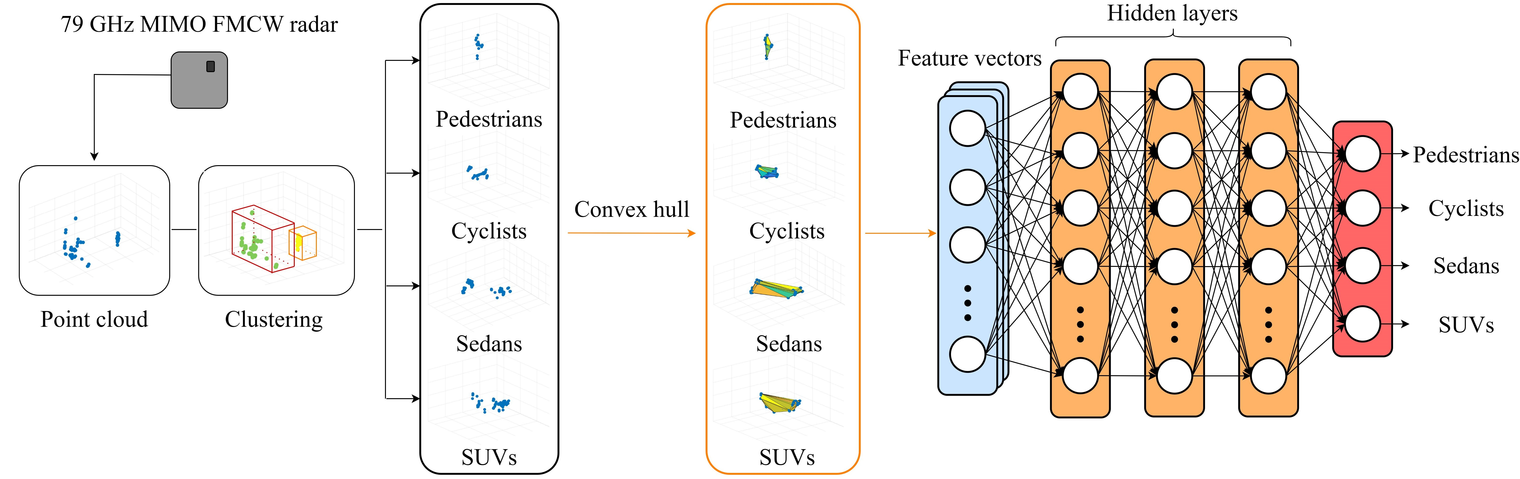
In this paper, we propose a method for efficient target classification based on the spatial features of the point cloud generated by using a high-resolution radar sensor. The frequency-modulated continuous wave radar sensor can estimate the distance and velocity of a target. In addition, the azimuth and elevation angle of the target can be estimated by using a multiple-input and multiple-output antenna system. Using the estimated distance, velocity, and angle, the 3D point cloud of target can be generated. From the generated point cloud, we extract the point cloud for each individual target using the density-based spatial clustering of application with noise method and a camera mounted on the radar sensor. Then, we define the convex hull boundaries that enclose these point clouds in both 3D and 2D spaces obtained by orthogonally projecting onto the $xy$, $yz$, and $zx$ planes. Using the vertices of convex hull, we calculate the volume of the targets and the areas in 2D spaces. Several feature points, including the calculated spatial information, are numerized and configured into feature vectors. We design an uncomplicated deep neural network classifier based on minimal input information to achieve fast and efficient classification performance. As a result, the proposed method achieved an average accuracy of 97.1%, and the time required for training was reduced compared to the method using only point cloud data and the convolutional neural network-based method.

1. Introduction

Automotive radar systems commonly use frequency-modulated continuous wave (FMCW) [1,2] technology. By employing frequency modulation on a continuous wave (CW) signal, it becomes possible to simultaneously estimate both the distance and velocity of a target. Moreover, a multiple-input and multiple-output (MIMO) antenna system [3,4], consisting of transmitting and receiving antenna elements, is used to estimate the angle of a target. Therefore, the recently developed concept of imaging radar can provide high-resolution point cloud images with enhanced imaging performance [5]. Target classification is a key technology directly related to driver safety in the driving assistance system. Traditionally, target classification in radar systems was mostly based on Doppler information [6,7,8]. However, recent advancements in radar sensors have enabled the acquisition of high-resolution point cloud data, leading to active research in target classification based on point cloud data. The authors in [9] proposed a method of classification and segmentation in driving environments using point clouds. As such, studies using various clustering techniques and classifiers were conducted to improve target classification performance [10,11,12]. In addition, the authors in [13] proposed a method for detecting and classifying the positions of dynamic road users by combining various classifiers. The authors in [14] proposed efficient real-time road user detection for multi-target traffic scenarios through FMCW measurement simulation.

Research on target classification methods using deep learning algorithms in radar systems has been recently conducted [15,16,17]. The authors of [15] applied a multi-view convolutional neural network (CNN) to the point clouds acquired using a high-resolution MIMO FMCW radar system for target classification. The authors in [16] proposed graph neural networks for radar object-type classification, which jointly process the radar reflection list and spectra. Also, the authors of [17] performed multiperson activity recognition tasks through a four-channel CNN classification model based on the Doppler, range, azimuth, and elevation features of the point cloud. Moreover, research has also been conducted using spatial features in conjunction with target information such as distance, velocity, and angle [18,19]. The authors of [18] transformed sparse point cloud data into radio frequency (RF) images to infer precise target shapes. In addition, the authors in [19] used the rolling ball method to extract accurate contour information from high-resolution radar point cloud data. In this paper, we focus on target classification in driving environments. We propose a method that effectively classifies stationary targets based on the spatial features of point clouds. We apply the density-based spatial clustering of applications with noise (DBSCAN) [20] method to cluster commonly encountered pedestrians, cyclists, sedans, and sports utility vehicles (SUVs) in road scenarios and define convex hull boundaries that enclose the point clouds in 3D and 2D space obtained by orthogonally projecting the data in three different directions (i.e., $xy$, $yz$, and $zx$ planes). Using the vertices of convex hull, we calculate the volume of the targets and the areas in 2D spaces. These spatial features are then complemented with the number of points in the point cloud. Additionally, we identify significant features that affect classification and validate the performance of the classification method with corresponding feature vectors.

In summary, the key contributions of our work can be outlined as follows:

• Through the proposed method, we obtain the vertices of convex hull that encloses the point cloud and extract spatial features by calculating the volume and areas in 3D and 2D space. Unlike conventional methods that merely cluster point cloud data, our approach considers the shape and perimeter of each cluster, enabling a deeper utilization of the target’s spatial features.
• The proposed spatial feature-based target classification method shows improved target classification performance compared to the case using spatial features extracted only with the DBSCAN method.
• By integrating spatial information into the classification process, our proposed method not only achieves higher accuracy but also reduces the training time compared to deep learning-based object classification methods that do not use spatial information.

The remainder of the paper is organized as follows. Section 2 provides an introduction to target estimation in the MIMO FMCW radar system, covering the fundamental concepts, and describing the experimental environment. In Section 3, we describe the process of extracting the vertices of the convex hull through the proposed method and the feature selection process for target classification. In Section 4, we describe the structure of the classifier. We also perform an analysis to identify the most significant features and evaluate the performance by comparing it with other target classification methods. Finally, we conclude this paper in Section 5.

2. Materials

2.1. Estimating Distance and Velocity of Targets with FMCW Radar System

In an automotive radar system, FMCW radar sensors can be used to simultaneously estimate the range, velocity, and angle of targets. Figure 1 shows the general block diagram of the MIMO FMCW radar system. The FMCW radar system sequentially transmits $N_p$ chirps, of which the frequency increases linearly in the time domain. $T_f$ denotes the frame time for transmitting the chirps, as shown in Figure 2.

Based on the returning echo signal from the target, we can estimate the velocity and distance of the kth target. The received signal is downconverted to a baseband signal by applying a frequency shift using a mixer and a low-pass filter. The baseband signal is transformed into a discrete-time signal through an analog-to-digital converter (ADC). The discrete-time signal can be expressed as

$$\begin{array}{c}\hfill \begin{array}{cc}\hfill \mathbf{x}[n,p]=& {\displaystyle \sum _{k=1}^{N_k}}{a}_k\exp \left[j2\pi \right\{\left(\frac{2\Delta f(R_k+v_{k}p\Delta t)}{c\Delta t}+\frac{2v_k{f}_c}{c}\right)n{T}_s\hfill \\ \hfill & +\frac{2f_c}{c}(R_k+v_{k}p\Delta t)\left\}\right]\hfill \end{array}\end{array}$$

(1)

where $f_c$, $\Delta f$, and $\Delta t$ represent the center frequency, bandwidth, and sweep time for each chirp, respectively. Moreover, $v_k$ and $R_k$ denote the velocity and distance of the kth target. Also, $N_k$ represents the number of targets, $a_k$ represents the amplitude of the kth baseband signal, and ${\psi }_0$ represents $2R_k{f}_c/c$. In addition, $n(n=1,2,\cdots ,N_n)$ represents the time sample index of each chirp, $p(p=1,2,\cdots ,N_p)$ represents the index of each chirp, and $T_s$ represents the sampling period. Applying the fast Fourier transform (FFT) with respect to the n-axis enables the estimation of the distance of the target, and applying the FFT with respect to the p-axis enables the estimation of the velocity of the target. This process is shown in Figure 2.

2.2. Target Angle Estimation Based on MIMO Antenna System

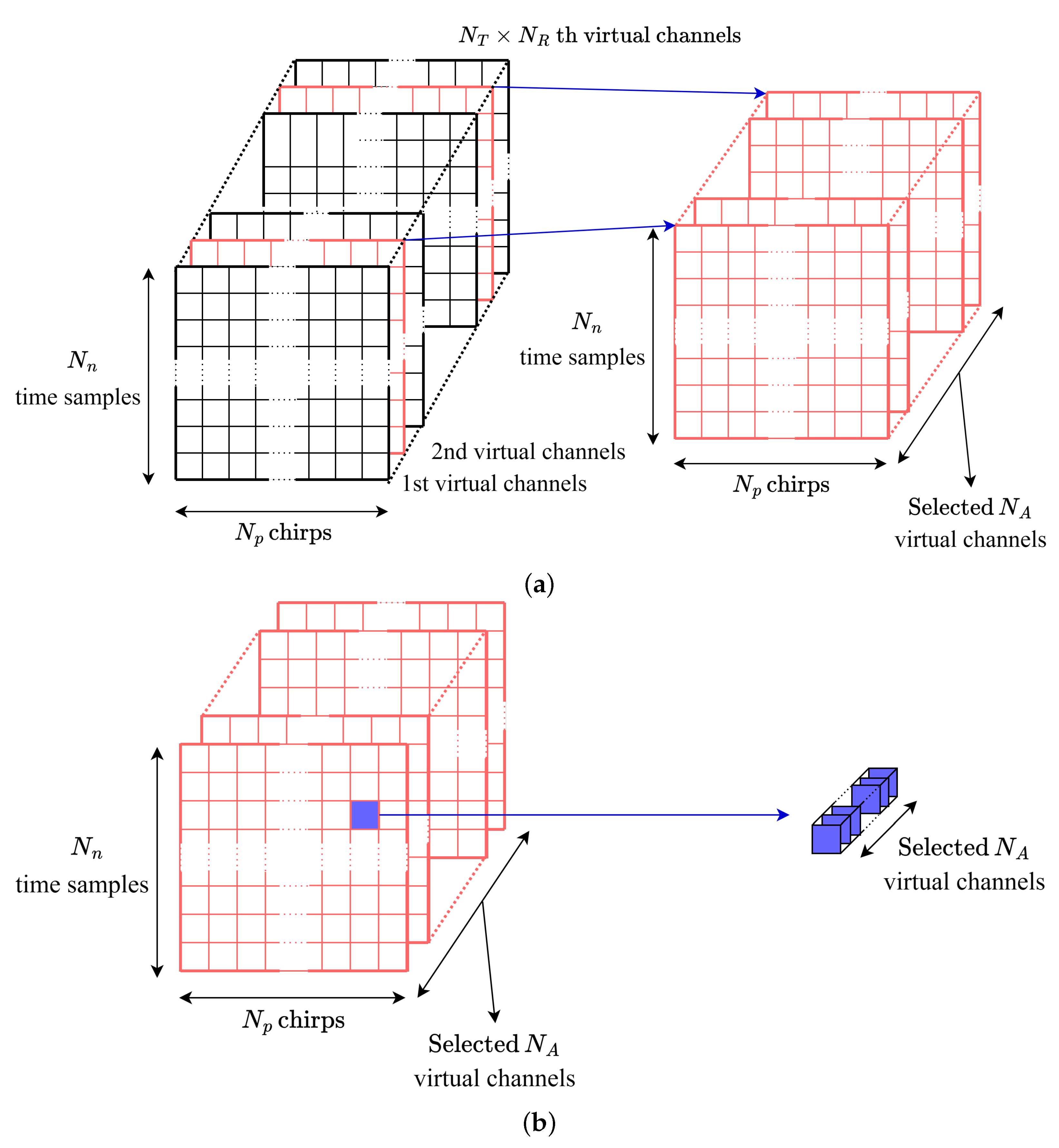
In an MIMO FMCW radar system, an array antenna can be used to determine both the azimuth and elevation angle of the target. Assuming that ${\theta }_k$ and ${\varphi }_k$ represent the azimuth and elevation angle, respectively, between the center of the antenna and the kth target, (1) can be expanded as

$$\begin{array}{c}\hfill \begin{array}{cc}\hfill \mathbf{x}[n,p,l,u]=& {\displaystyle \sum _{k=1}^{N_k}}{a}_k\exp \left[j2\pi \right\{\left(\frac{2\Delta f(R_k+v_{k}p\Delta t)}{c\Delta t}+\frac{2v_k{f}_c}{c}\right)n{T}_s\hfill \\ \hfill & +\frac{f_c{d}_{t,a}sin{\theta }_k}{c}(l-1)+\frac{f_c{d}_{r,a}sin{\theta }_k}{c}(u-1)\hfill \\ \hfill & +\frac{f_c{d}_{t,e}sin{\varphi }_k}{c}(l-1)+\frac{f_c{d}_{r,e}sin{\varphi }_k}{c}(u-1)\hfill \\ \hfill & +\frac{2f_c}{c}(R_k+v_{k}p\Delta t)\left\}\right]\hfill \end{array}\end{array}$$

(2)

where $d_{t,a}$ and $d_{t,e}$ represent the distances between the transmitting antenna elements in the azimuth and elevation directions, while $d_{r,a}$ and $d_{r,e}$ represent the distances between the receiving antenna elements. In the MIMO antenna system, $l(l=1,2,\cdots ,N_T)$ represents the index of the transmitting antenna elements, and $u(u=1,2,\cdots ,N_R)$ represents the index of the receiving antenna elements. Using these elements, $N_T\times N_R$ virtual channels can be generated. When $N_T\times N_R$ receiving channels are generated, a total of $N_T\times N_R$ 2D FFT results are obtained.

Assuming that the number of receiving channels arranged in the azimuth direction is $N_A$, and representing the 2D FFT results corresponding to the kth target in each virtual channel as $t_k$ and $r_k$, we obtain a total of $N_A$ sampled values. This process is shown in Figure 3, and the signal vector can be expressed as

$$\begin{array}{c}\hfill {\mathbf{X}}_A=\left[\begin{array}{c}{X}_1\left[t_k,r_k\right]\\ X_2\left[t_k,r_k\right]\\ ⋮\\ X_{N_A}\left[t_k,r_k\right]\end{array}\right]\end{array}$$

(3)

The spectrum-based beamforming technique, the Bartlett angle estimation algorithm [21], is employed using the signal spectrum from (3). By multiplying ${\mathbf{X}}_A$ with the Hermitian transpose of ${\mathbf{X}}_A$, denoted as ${\mathbf{X}}_A^H$, we generate a correlation matrix. The normalized pseudospectrum can be expressed as

$$\begin{array}{c}\hfill P_A\left(\theta \right)=\frac{1}{N_A}\frac{{\mathbf{a}}_A^H\left(\theta \right){\mathbf{X}}_A{\mathbf{X}}_A^H{\mathbf{a}}_A\left(\theta \right)}{{\mathbf{a}}_A^H\left(\theta \right){\mathbf{a}}_A\left(\theta \right)}\end{array}$$

(4)

where ${\mathbf{a}}_A\left(\theta \right)$ is the steering vector that takes into account the distance between the receiving channels in the azimuth direction. Similarly to estimating the azimuth angle of the target, the elevation angle can be estimated by assuming the number of sampled values containing information in the elevation direction as $N_E$. The corresponding steering vector is represented as ${\mathbf{a}}_E\left(\varphi \right)$.

2.3. 3D Target Generation Using FMCW Radar System

2.3.1. Radar Sensor Used in Measurements

For this experiment, we used a radar sensor manufactured by Bitsensing inc., Seoul, Republic of Korea, known as the 79 GHz AIR 4D [22]. The radar sensor operated at a center frequency of 79 GHz with a bandwidth of 1500 MHz, resulting in a range resolution of 10 cm, which is determined by $c/2B$. The system consisted of 32 chirps, with each chirp comprising 1024 time samples. It features 12 transmitting antenna elements and 16 receiving antenna elements. The frame time is set to 100 ms. The velocity resolution is 1.9 cm/s, and the angular resolutions for elevation and azimuth are 5^∘ and 2^∘, respectively. The specifications of the radar sensor are summarized in

Table 1. Characteristics of the MIMO FMCW radar system.

Parameter	Value
Center frequency, $f_c$	79 GHz
Bandwidth, $\Delta f$	1500 MHz
Number of transmitting antenna elements, $N_T$	12
Number of receiving antenna elements, $N_R$	16
Number of chirps, $N_p$	32
Number of time samples in each chirp, $N_n$	1024
Frame time, $T_f$	100 ms
Range resolution, $\Delta R$	10 cm
Velocity resolution, $\Delta v$	1.9 cm/s
Azimuth angular resolution, $\Delta \theta$	2∘
Elevation angular resolution, $\Delta \varphi$	5∘

.

2.3.2. Measurement Scenarios

We obtained data from different targets commonly encountered during road driving, including pedestrians, cyclists, sedans, and SUVs from radar sensors. Because of the dynamic nature of non-stationary targets, where spatial features can change over time, we focused our analysis on stationary targets to clearly analyze the impact of spatial features without complicating effects of velocity. The length, height, and width of the observed stationary targets are provided in the

Table 2. Length, height, and width of each target class.

Target Class	Length (mm)	Height (mm)	Width (mm)
Pedestrians	280–540	1680–1830	575–645
Cyclists	1680–1760	1750–1900	500–580
Sedans	4588–4995	1470–1485	1860–1870
SUVs	4410–4750	1020–1715	1830–1930

. The radar sensor was positioned at a height of 60 cm above the ground surface. To classify stationary targets from various angles, the angle and distance between the radar and the target were adjusted, and data were acquired by measuring 200 frames at 14 different points as shown in Figure 4a. We also obtained data for cases where targets are adjacent (e.g., cyclists and pedestrians, SUVs and pedestrians within 1 m) to ensure that they can be applied to complex environments. Measurements were taken over 200 frames, identical to when observing stationary targets at 6 different points, as shown in Figure 4b. In this case, we empirically determined that the maximum distance between point clouds associated with a specific target is approximately 70 cm. Considering the radar’s range resolution, we adjusted the distance hyperparameter of the DBSCAN algorithm to 80 cm and set the minimum number of points required for a cluster to 4. Based on these hyperparameters, we ensured a minimum separation of 1 m between targets in all experiments, which were conducted in an outdoor environment free from obstructions. In addition, we merged point clouds collected from multiple sensor positions into a unified dataset. Using this integrated dataset, we trained our classification model to accurately classify targets regardless of the direction from which they are observed.

2.4. Point Cloud Refinement Process

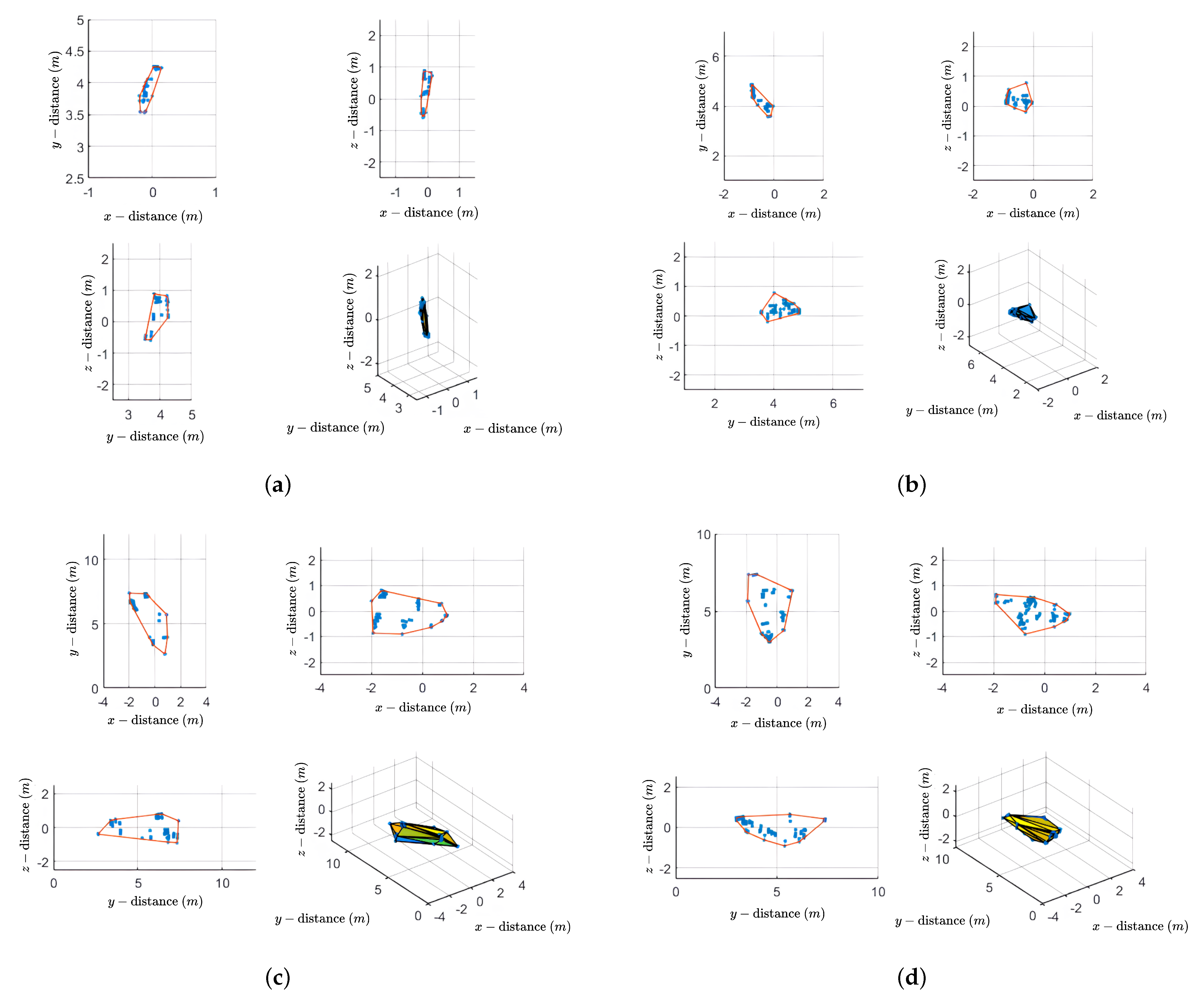
Through the use of the estimated distance and angle parameters (i.e., $R_k$, ${\theta }_k$, and ${\varphi }_k$) obtained from Section 2.1 and Section 2.2, the spatial location of the targets in 3D space can be estimated. We used the DBSCAN method and a camera mounted on a radar sensor to define a virtual bounding box (i.e., the smallest cuboid that encloses the point cloud) and consider all points outside this area as outliers, displaying only the point cloud within this area. By adjusting the hyperparameters (i.e., the number of points and clustering size) of the DBSCAN method, it was possible to cluster targets even in complex environments. Figure 5 represents point clouds in the $xy$, $yz$, and $zx$ planes and 3D space, respectively, starting from the top left. Also, Figure 6 shows the clustering results for multiple targets, with the point clouds for each target displayed in different colors according to the clustering, as shown in Figure 6b.

3. Methods

In this section, we propose a method of extracting vertices from the convex hull of the point cloud. The process of obtaining the volume and areas of the target through the extracted vertices is explained, and other features for target classification are considered.

3.1. Process for Extracting Vertices of a Convex Hull

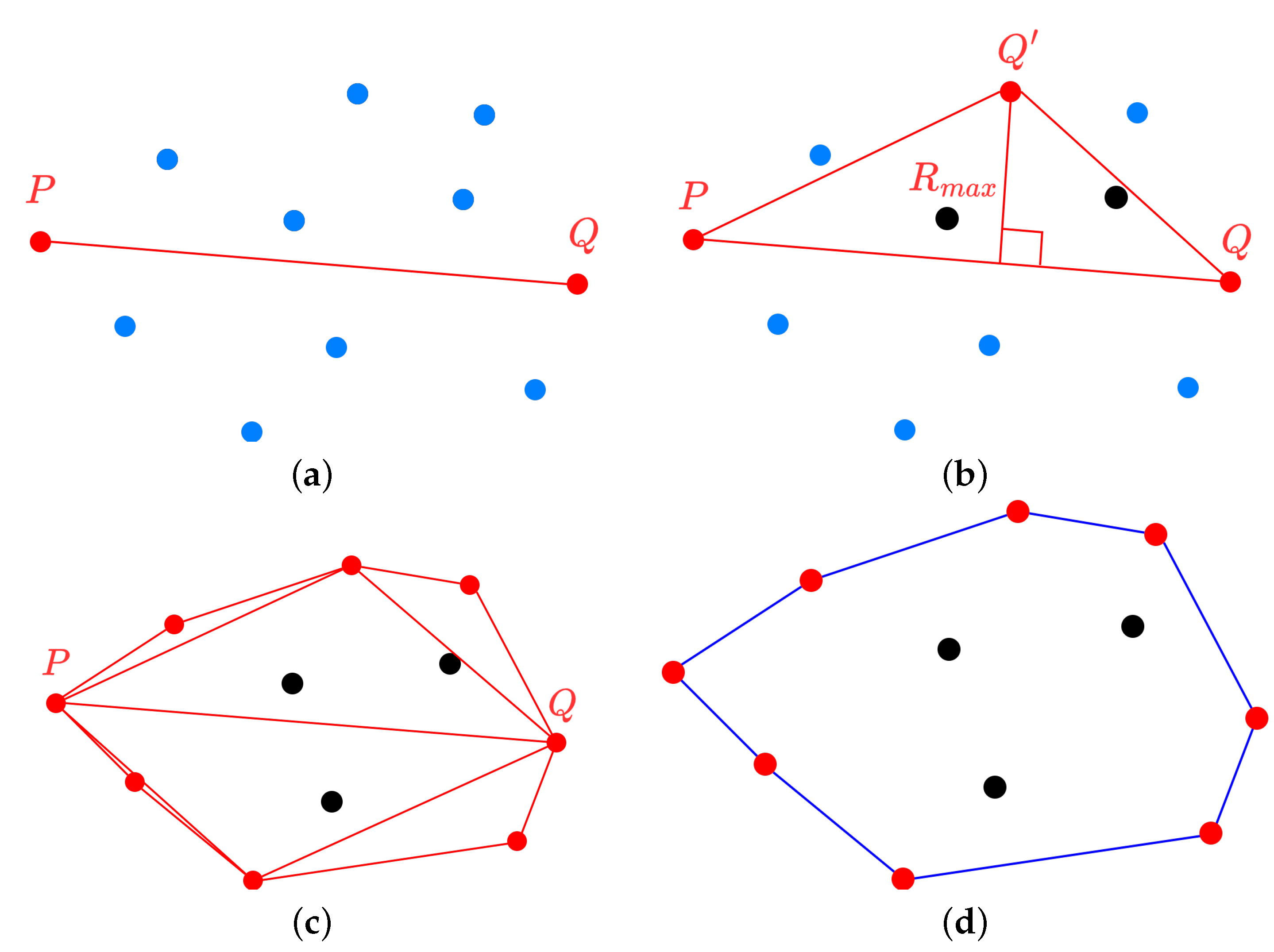
We propose a method for extracting the convex hull’s vertices of a finite set of points in n-dimensional space using the divide-and-conquer method [23,24], based on the point clouds generated through the MIMO FMCW radar system. Figure 7 shows the process of selecting vertices to form a convex hull: red dots represent the selected vertices, blue dots represent points under consideration, and black dots represent points excluded from consideration. Also, the red line represents the line generated by repeating Figure 7a and Figure 7b, and the blue line represents the final boundary of the convex hull. Using the two furthest points in the 2D point cloud as reference points as shown in Figure 7a, the point cloud is divided into two groups according to a baseline connecting these reference points. For each group of points, we find the furthest point that is orthogonal to the baseline. As shown in Figure 7b, this point becomes a new vertex, forming a triangle with the reference point. Points inside the triangle cannot be part of the convex hull and can, therefore, be ignored in subsequent steps. Then, continue to recursively apply the previous two steps to the lines created by the new sides of the triangle. By repeating these two steps recursively on the two lines formed by the new sides of the triangle until no more points remain, the line segments depicted in Figure 7c are created. As a result, the selected vertices form a convex hull, as shown in Figure 7d. We apply the proposed method to the point clouds generated in Section 2.3.2. Figure 8 shows the application of the proposed method to Figure 5. In Figure 8, the color intensity of the triangles corresponds to their relative height within the point cloud, with darker shades indicating lower elevations.

3.2. Features Selection with Proposed Method

To calculate the areas, we used the coordinates of the vertices of the convex hull. The equation for calculating the areas of the obtained vertices can be expressed as

$$\begin{array}{cc}\hfill & A_{xy}=\frac{1}{2}\left|{\displaystyle \sum _{i=1}^{m-1}}{x}_i{y}_{i+1}+x_m{y}_1-{\displaystyle \sum _{i=1}^{m-1}}{x}_{i+1}{y}_i-x_1{y}_m\right|\hfill \end{array}$$

(5)

$$\begin{array}{cc}\hfill & A_{yz}=\frac{1}{2}\left|{\displaystyle \sum _{i=1}^{m-1}}{y}_i{z}_{i+1}+y_m{z}_1-{\displaystyle \sum _{i=1}^{m-1}}{y}_{i+1}{z}_i-y_1{z}_m\right|\hfill \end{array}$$

(6)

$$\begin{array}{cc}\hfill & A_{zx}=\frac{1}{2}\left|{\displaystyle \sum _{i=1}^{m-1}}{z}_i{x}_{i+1}+z_m{x}_1-{\displaystyle \sum _{i=1}^{m-1}}{z}_{i+1}{x}_i-z_1{x}_m\right|\hfill \end{array}$$

(7)

where the coordinates of x, y, and z in (5)–(7) represent the coordinates of the vertices forming the convex hull in each of the three different planes and are conditioned on the following equation:

$$\begin{array}{cc}\hfill & x_{n+1}=x_1,x_0=x_n,y_{n+1}=y_1,y_0=y_n,z_{z+1}=z_1,z_0=z_n\hfill \end{array}$$

(8)

Similarly, the volume of the convex hull in 3D space can also be calculated. The equation can be expressed as

$$\begin{array}{c}\hfill V_{xyz}=\frac{1}{6}{\displaystyle \sum _{i=1}^{m-1}}{\displaystyle \sum _{j=i+1}^m}{\displaystyle \sum _{k=j+1}^m}{\mathbf{v}}_i\times ({\mathbf{v}}_j-{\mathbf{v}}_i)\times ({\mathbf{v}}_k-{\mathbf{v}}_i)\end{array}$$

(9)

where $\mathbf{v}$ represents the coordinates of the vertices that form the convex hull, and m represents the number of vertices. In addition, we considered the number of points in the point cloud and denoted it as $N_{\mathrm{points}}$.

4. Results

In this section, we describe structure of the deep neural network (DNN) for target classification and configure the feature vectors from the features considered in Section 3.2, through the performance evaluation. Furthermore, we compare the performance with other target classification methods that do not use spatial information.

4.1. The Structure of the DNN for Target Classification

DNNs have the advantage of enhanced training ability compared to artificial neural networks, as they have multiple hidden layers. As a result, there have been numerous studies applying radar sensor data to DNNs. The authors in [25] proposed a machine learning-based method to classify pedestrians using automotive radar. They used the DBSCAN method for clustering detected targets and calculated features to identify targets belonging to the same moving object. In addition, the authors in [26] proposed a method to improve the target classification accuracy of automotive radar sensors by directly applying deep convolutional neural networks to the region of interest on the radar spectrum.

Figure 9 shows the structure of the DNN for target classifications. The DNN model used in this paper consists of three hidden layers, and each layer is composed of 30 nodes. The activation functions of the hidden layers are connected in the order of sigmoid, hyperbolic tangent, and hyperbolic tangent. Finally, they pass through the softmax layer and output layer to generate the output. Training is carried out by feedforward, where the nodes of the input layer are multiplied by weight and added with bias as they are passed to the next layer. Then, the process passes through the activation function and reaches the output layer. If the training is incorrect, the process is adjusted by correcting the gradient of the nodes through error backpropagation.

For the input, we started with five types of features (i.e., the areas of the convex hull observed from three directions, volume, and the number of points) and empirically reduced them to the most significant features. The output types of targets were fixed to pedestrians, cyclists, sedans, and SUVs. We obtained a total of 11,200 feature vectors for different types of pedestrians, cyclists, sedans, and SUVs. The input data are divided with 75% of the data allocated to training and 25% allocated to testing. The maximum number of epochs for training is set to 1500, where each epoch represents one complete iteration over the entire feature vector. The training data are further divided into random independent samples, with 70% for training, 15% for validation, and 15% for testing purposes.

4.2. Performance Evaluation

For efficient target classification, we constructed feature vectors for the two cases and evaluated their performance. First, the performance was evaluated considering all five types of features considered in Section 3.2. Then, the classification performance was evaluated using only the areas and volume of the target obtained through the proposed method, excluding the number of points. The average classification accuracy is presented in

Table 3. Classifier evaluation for different feature vectors.

Feature Vectors	Average Classification Accuracy
${\mathbf{f}}_0=(A_{xy},A_{yz},A_{zx},V_{xyz},N_{\mathrm{points}})$	91.7%
${\mathbf{f}}_1=(A_{xy},A_{yz},A_{zx},V_{xyz})$	87.0%

.

4.2.1. Classification Using All Features

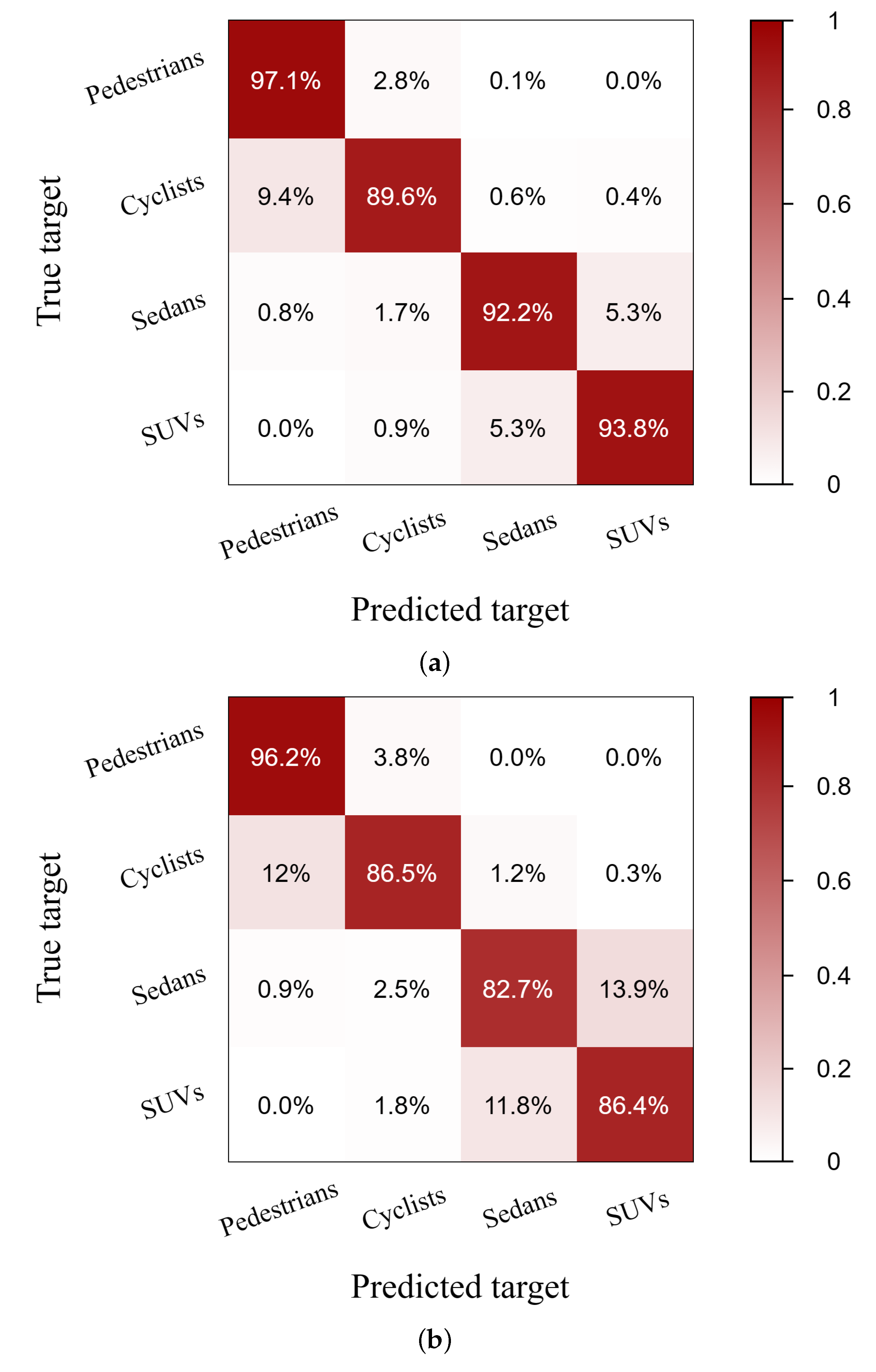
As shown in Table 3, the feature vector consisting of all five features considered is ${\mathbf{f}}_0$. Figure 10a shows the confusion matrix for ${\mathbf{f}}_0$. As shown in Figure 10a, pedestrians showed the highest classification accuracy at 97.1%. In contrast, the accuracy of prediction for cyclists was relatively low at 89.6%, and the highest error rate was 9.4% when cyclists were confused with pedestrians. The average classification accuracy of all features was 91.7%.

4.2.2. Classification Using Selected Features

To determine which features significantly affect classification performance, we constructed a feature vector ${\mathbf{f}}_1=(A_{xy},A_{yz},A_{zx},V_{xyz})$. Figure 10b represents the confusion matrix obtained from the feature vector ${\mathbf{f}}_1$. The classification performance decreased by 4.7% when the number of points comprising the targets was removed. Despite a slight decrease in classification performance, the spatial features of areas and volume exhibited a high classification accuracy of 87.0%. This finding confirms that these spatial features are significant factors in the classification process.

4.3. Comparison of Spatial Features from a Virtual Bounding Box and the Proposed Method

To evaluate the performance of the proposed method, we compared it with the use of spatial features extracted by a virtual bounding box. In Section 2.4, we used the camera mounted on the radar sensor to define a virtual bounding box corresponding to the targets. The spatial features extracted in Section 4.2.2 (i.e., $A_{xy}$, $A_{yz}$, $A_{zx}$, and $V_{xyz}$) were replaced by the area and volume obtained by orthogonally projecting the virtual bounding box in three different directions. The feature vectors were organized in the form of ${\mathbf{f}}_0$, which yields the highest classification accuracy.

Table 4. Classification accuracy for different clustering methods.

	Methods	DBSCAN + Proposed	DBSCAN
Target Class
Pedestrians		97.1%	94.3%
Cyclists		89.6%	84.7%
Sedans		92.2%	91.5%
SUVs		93.8%	92.2%

shows the classification accuracy when using spatial features from virtual bounding boxes and the proposed method. The accuracy of predicting pedestrians was improved by 2.8% when using the feature vectors processed with the proposed method. Particularly, the accuracy of predicting cyclists was improved by 4.9%, and the overall average classification accuracy was enhanced by 3.5%.

4.4. Comparison with Other Target Classification Methods

In this section, we compare the proposed method with other deep learning-based target classification methods. We compare the performance of the proposed method against following models that are widely used for target classification: PointNet and SqueezeNet. PointNet uses the coordinate information of the point cloud as the input, while SqueezeNet uses the point cloud images from the $xy$, $yz$, and $zx$ planes. Figure 11 shows the confusion matrices for target classification result. The training time was computed based on the Intel Core i7-9750H CPU (Intel Corporation, Santa Clara, CA, USA), GeForce GTX 1650 GPU (NVIDIA Corporation, Santa Clara, CA, USA), and Samsung 16 GB RAM (Samsung Electronics, Suwon, Republic of Korea).The required training time and average accuracy are shown in

Table 5. Performance comparison with proposed method, PointNet, and SqueezeNet.

Target Classification Method	Proposed	PointNet	SqueezeNet
Average classification accuracy	91.7%	67.9%	91.1%
Time required for training	2 m 3 s	8 m 12 s	46 m 17 s

. As shown in Table 5, the average classification accuracies when using PointNet and SqueezeNet were 67.9% and 91.1%, respectively. Compared to the proposed method, the accuracies of each method were 23.8% and 0.6% lower, respectively. Additionally, when comparing the time required for training, the proposed method showed a faster training time than the other two methods. As a result, the proposed method showed the highest performance relative to the required training time compared to target classification methods that do not use spatial information.

Moreover, we also compared the proposed method with other research methods that classify targets using spatial features, which are currently attracting attention. The first method mainly converts the sparse point cloud into an RF image to obtain the accurate shape of the target. For instance, PointNet can accurately capture the local structure and geometry of a vehicle from dense point clouds. However, millimeter-wave radar only captures the vehicle’s edge in the point cloud, leaving other regions unknown. Consequently, PointNet cannot accurately infer the shape and category of vehicles from these sparse point clouds. Therefore, the researchers noted that RF images from automotive radars provide more information for target detection than point clouds. However, they contain significant noise, increasing neural network complexity and slowing down processing. In contrast, radar point clouds offer simpler data collection, lower noise, and faster processing through peak detection algorithms such as constant false alarm rate. Therefore, our proposal used radar point clouds to not only identify clusters but also accurately describe the outlines of these clusters, thereby improving the general accuracy of deep learning even for sparse point clouds. The second method is to estimate target outline information from a high-resolution target point group using the rolling ball technique. This technique is effective in detailing the fine contours of radar point cloud data, similar to the proposed method. Parameters with optimal results must be set depending on the type of target, but the proposed method does not require parameter adjustment depending on the type of target. In addition, our method using convex hull processing is less sensitive to noise and outliers compared to rolling ball methods because the convex hull naturally excludes extremes. This property also improves computational efficiency, making convex hull calculations relatively efficient even for large data sets, making them suitable for computer vision and machine learning tasks. These features highlight the advantages of our approach over existing methods, providing a strong foundation for improved target classification and tracking in automotive radar applications.

5. Conclusions

In this paper, we proposed a DNN-based target classification method for high-resolution automotive radar systems. From the raw data obtained by the MIMO FMCW radar sensor, we processed and transformed it into point clouds representing four different target types: pedestrians, cyclists, sedans, and SUVs. Then, we extracted the vertices of the point cloud surrounding the targets in 3D and 2D space. Using the vertices constituting the convex hull of the targets, we obtained more accurate spatial information regarding the target. We configured the feature vectors by incorporating the obtained spatial features along with the number of points. Then, we evaluated the classification performance of the DNN classifier using the selected features. Finally, we compared the proposed method with other target classification methods that do not use spatial information, and the proposed target classification method exhibited faster training time and higher classification accuracy.

References

- Winkler, V. Range Doppler detection for automotive FMCW radars. In Proceedings of the European Microwave Conference, Munich, Germany, 9–12 October 2007; pp. 166–169. [Google Scholar]
- Patole, S.M.; Torlak, M.; Wang, D.; Ali, M. Automotive radars: A review of signal processing techniques. IEEE Signal Process. Mag. 2017, 34, 22–35. [Google Scholar] [CrossRef]
- MIMO Radar. Available online: https://www.ti.com/lit/an/swra554a/swra554a.pdf (accessed on 3 March 2024).
- Wang, X.; Wan, L.; Huang, M.; Shen, C.; Zhang, K. Polarization channel estimation for circular and non-circular signals in massive MIMO systems. IEEE J. Sel. Top. Signal Process. 2019, 13, 1001–1016. [Google Scholar] [CrossRef]
- Jiang, M.; Xu, G.; Pei, H.; Feng, Z.; Ma, S.; Zhang, H.; Hong, W. 4D high-resolution imagery of point clouds for automotive mmWave radar. IEEE Trans. Intell. Transp. Syst. 2023, 25, 1–15. [Google Scholar]
- Rizik, A.; Randazzo, A.; Vio, R.; Delucchi, A.; Chible, H.; Caviglia, D.D. Feature extraction for human-vehicle classification in FMCW radar. In Proceedings of the 26th IEEE International Conference on Electronics, Circuits and Systems (ICECS), Genoa, Italy, 27–29 November 2019; pp. 131–132. [Google Scholar]
- Rohling, H.; Heuel, S.; Ritter, H. Pedestrian detection procedure integrated into an 24 GHz automotive radar. In Proceedings of the IEEE Radar Conference, Arlington, VA, USA, 10–14 May 2010; pp. 1229–1232. [Google Scholar]
- Villeval, S.; Bilik, I.; Gürbuz, S.Z. Application of a 24 GHz FMCW automotive radar for urban target classification. In Proceedings of the IEEE Radar Conference, Cincinnati, OH, USA, 19–23 May 2014; pp. 1237–1240. [Google Scholar]
- Charles, R.Q.; Su, H.; Kaichun, M.; Guibas, L.J. Pointnet: Deep learning on point sets for 3D classification and segmentation. In Proceedings of the IEEE Conference on Computer Vision and Pattern Recognition (CVPR), Honolulu, HI, USA, 21–26 July 2017; pp. 652–660. [Google Scholar]
- Zhao, Z.; Song, Y.; Cui, F.; Zhu, J.; Song, C.; Xu, Z.; Ding, K. Point cloud features-based kernel SVM for human-vehicle classification in millimeter wave radar. IEEE Access 2020, 8, 26012–26021. [Google Scholar] [CrossRef]
- Palffy, A.; Dong, J.; Kooij, J.F.P.; Gavrila, D.M. CNN based road user detection using the 3D radar cube. IEEE Robot. Autom. Lett. 2020, 5, 1263–1270. [Google Scholar] [CrossRef]
- Kim, Y.; Alnujaim, I.; Oh, D. Human activity classification based on point clouds measured by millimeter wave MIMO radar with deep recurrent neural networks. IEEE Sens. J. 2021, 21, 13522–13529. [Google Scholar] [CrossRef]
- Scheiner, N.; Kraus, F.; Appenrodt, N.; Dickmann, J.; Sick, B. Object detection for automotive radar point clouds—A comparison. AI Perspect. 2021, 3, 1–23. [Google Scholar] [CrossRef]
- Wengerter, T.; Pérez, R.; Biebl, E.; Worms, J.; O’Hagan, D. Simulation of urban automotive radar measurements for deep learning target detection. In Proceedings of the IEEE Intelligent Vehicles Symposium (IV), Aachen, Germany, 4–9 June 2022; pp. 309–314. [Google Scholar]
- Kwak, S.; Kim, H.; Kim, G.; Lee, S. Multi-view convolutional neural network-based target classification in high-resolution automotive radar sensor. IET Radar Sonar Navig. 2023, 17, 15–23. [Google Scholar] [CrossRef]
- Saini, L.; Acosta, A.; Hakobyan, G. Graph neural networks for object type classification based on automotive radar point clouds and spectra. In Proceedings of the IEEE International Conference on Acoustics, Speech and Signal Processing (ICASSP), Rhodes Island, Greece, 4–10 June 2023; pp. 1–5. [Google Scholar]
- Wu, Z.; Cao, Z.; Yu, X.; Zhu, J.; Song, C.; Xu, Z. A novel multiperson activity recognition algorithm based on point clouds measured by millimeter-wave MIMO radar. IEEE Sens. J. 2023, 23, 19509–19523. [Google Scholar] [CrossRef]
- Lu, G.; He, Z.; Zhang, S.; Huang, Y.; Zhong, Y.; Li, Z.; Han, Y. A novel method for improving point cloud accuracy in automotive radar object recognition. IEEE Access 2023, 11, 78538–78548. [Google Scholar] [CrossRef]
- Tan, B.; Ma, Z.; Zhu, X.; Li, S.; Zheng, L.; Huang, L.; Bai, J. Tracking of multiple static and dynamic targets for 4D automotive millimeter-wave radar point cloud in urban environments. Remote Sens. 2023, 15, 2923. [Google Scholar] [CrossRef]
- Ester, M.; Kriegel, H.-P.; Sander, J.; Xu, X. A density-based algorithm for discovering clusters in large spatial databases with noise. In Proceedings of the 2nd International Conference on Knowledge Discovery and Data Mining (KDD’96), Portland, OR, USA, 2 August 1996; pp. 226–231. [Google Scholar]
- Richmond, C.D. Capon and Bartlett Beamforming: Threshold Effect in Direction-of-Arrival Estimation Error and on the Probability of Resolution; Technical Report; Massachusetts Institute of Technology, Lincoln Laboratory: Lexington, MA, USA, 2005; pp. 1–80. [Google Scholar]
- AIR 4D. Available online: http://bitsensing.co.kr/solution/mobility (accessed on 3 March 2024).
- Greenfield, J.S. A Proof for a Quickhull Algorithm; Technical Report; Syracuse University: Syracuse, NY, USA, 1990; pp. 1–19. [Google Scholar]
- Barber, C.B.; Dobkin, D.P.; Huhdanpaa, H. The quickhull algorithm for convex hulls. ACM Trans. Math. Softw. 1996, 22, 469–483. [Google Scholar] [CrossRef]
- Prophet, R.; Hoffmann, M.; Ossowska, A.; Malik, W.; Sturm, C.; Vossiek, M. Pedestrian classification for 79 GHz automotive radar systems. In Proceeding of the IEEE Intelligent Vehicles Symposium (IV), Changshu, China, 26–30 June 2018; pp. 1265–1270. [Google Scholar]
- Patel, K.; Rambach, K.; Visentin, T.; Rusev, D.; Pfeiffer, M.; Yang, B. Deep learning-based object classification on automotive radar spectra. In Proceeding of the IEEE Radar Conference (RadarConf), Boston, MA, USA, 22–26 April 2019; pp. 1–6. [Google Scholar]
Figure 1.
Block diagram of the MIMO FMCW radar system.
Figure 2.
Process of estimating distance and velocity based on the transmitted and received signals from the FMCW radar system.
Figure 3.
Angle estimation of the azimuth direction. (a) selection of receiving channels and (b) selection of the time sample index and chirp index where the target is located.
Figure 4.
Measurement scenarios (a) for individual targets and (b) for multiple targets.
Figure 5.
Generated point clouds in the , , and planes and 3D space for (a) pedestrians, (b) cyclists, (c) sedans, and (d) SUVs.
Figure 6.
Generated 3D point cloud data in multi-target scenario (a) before applying clustering and (b) after applying clustering.
Figure 7.
Process of selecting the vertices that form a convex hull using the proposed method: (a) set a baseline connecting the two furthest points, (b) form a triangle by selecting the point that is orthogonally furthest from the baseline, (c) The line segments and selected vertices that are generated by repeating the previous process, and (d) final selected vertices and convex hull.
Figure 8.
Applied proposed method to the point clouds (a) for pedestrians, (b) for cyclists, (c) for sedans, and (d) for SUVs.
Figure 9.
Block diagram of the proposed DNN for target classification.
Figure 10.
Confusion matrices based on (a) and (b) .
Figure 11.
Confusion matrices in (a) the PointNet and (b) the SqueezeNet.