Multi-Scenario Simulation of Land System Change in the Guangdong–Hong Kong–Macao Greater Bay Area Based on a Cellular Automata–Markov Model

Abstract

As one of the four major bay areas in the world, the Guangdong–Hong Kong–Macao Greater Bay Area (GBA) is a highly integrated mega urban agglomeration and its unparalleled urbanization has induced prominent land contradictions between humans and nature, which hinders its sustainability and has become the primary concern in this region. In this paper, we probed the historical characteristics of land use and land cover change (LUCC) in the GBA from 2005 to 2015, and forecasted its future land use pattern for 2030, 2050, and 2070, using a cellular automata–Markov (CA–Markov) model, under three typical tailored scenarios, i.e., urban development (UD), cropland protection (CP), and ecology security (ES), for land use optimization. The major findings are as follows: (1) The encroachments of build-up land on the other land uses under rapid urbanization accounted for the leading forces of LUCCs in the past decade. Accordingly, the urban sprawl was up to 1441.73 km² (23.47%), with cropland, forest land, and water areas reduced by 570.77 km² (4.38%), 526.05 km² (1.76%), and 429.89 km² (10.88%), respectively. (2) Based on the validated CA–Markov model, significant differences are found in future land use patterns under multiple scenarios, with the discrepancy magnified over time and driven by different orientations. (3) Through comprehensive comparisons and tradeoffs, the ES scenario mode seems optimal for the GBA in the next decades, which optimizes the balance between socio-economic development and ecological protection. These results serve as an early warning for future land problems and can be applied to land use management and policy formulation to promote the sustainable development of the GBA.

1. Introduction

Land use and land cover change (LUCC) is an important factor altering ecosystems and the natural balance at regional and global scales and has intensified in recent decades due to human interventions [1,2,3]. Under the general trend of global urbanization, LUCC occurs frequently and manifests as the conversion from natural covers to artificial surfaces, especially in developing countries [4,5,6]. It breaks the balance of the Earth’s system and has led to a series of subsequent effects, such as land degradation, climate change, eco-environment deterioration, biodiversity loss, food security, etc. [7,8,9,10]. Thus, how to rationally manage limited land resources to balance socio-economic development and ecological needs is at the core of sustainable development.

Land use simulations illuminate the dynamic mechanism of land systems and anthropogenic–natural impacts, by qualitatively or quantitatively modeling land use conversions in the past and using the underlying driving forces to forecast future land use demand and spatial allocation at various temporal or spatial scales [11,12,13]. To effectively model LUCCs, numerous land use simulation models have been put forward in the past decades. According to the working scheme, they can be summarized into three main kinds: the quantitative prediction model, spatial simulation model, and coupling model of quantitative prediction and spatial simulation [3,14].

The quantitative prediction model mainly focuses on land use demand estimation to give a possible area for each land use in the future, but ignores the spatial distributions of various land uses for land allocation guidance. The representative methods include the logistic regression (LR) model [15,16], system dynamic (SD) model [17,18], Markov chain model [19,20], and so on. The spatial simulation model pays more attention to the interactions between geographical units and spatial drivers to estimate the growth probability of different land uses in each geographical unit, with the cellular automata (CA) model [21,22], conversion of land use and its effects (CLUE) model [23,24], and agent-based model [25,26] as typical representations. Such methods directly provide land allocations, but with a limited ability to model global influencing factors, like policy, economy, etc. The coupling model takes full advantages of the above two methods to give more accurate and comprehensive simulation results and has been a common strategy in land use simulation [27,28]. The typical examples are the CA–Markov model [29,30], CA–SD model [31,32], and Dyna–CLUE–Markov model [33,34]. Among them, the CA–Markov model combines the advantages of the CA and Markov chain models to simultaneously predict the spatial pattern and temporal trend and is suitable for the complex change simulation of multiple land uses, which has been widely applied to LUCC analysis [35,36].

The scenario simulation based on the above models gives reasonable forecasting consequences of land use demand and spatial allocation in the future, which enables strategical land use optimization and scientific decision-making [37,38]. In the past years, extensive LUCC simulation research projects under certain scenarios have been carried out at various scales, which greatly improves the understanding of the comprehensive influences of anthropogenic processes and policy formulation on land system evolution. For instance, Han et al. combined CLUE-S and Markov models to conduct a development-and-protection scenario simulation for Beijing during the period between 2010 and 2020 and found that the conversion from arable land to build-up land was the major feature, especially for mountainous areas [39]. Zou et al. explored a sustainable land use model in Nan’an City through land use conflict (LUC) management, with seven conflict levels and 16 LUC zones considered, to draw a conclusion that differentiated strategies might be adopted to relieve the conflicts in various LUC zones [40]. In addition, Yang et al. investigated LUCCs in the Beijing–Tianjin–Hebei region during the period between 2000 and 2015 and projected its future land use pattern in 2030 based on the Dyna–CLUE model under three tailored scenarios, with the results indicating that the ecology security scenario is optimal for regional planning [41].

China has undergone significant urbanization in the past decades, with urbanization accompanied by intense expansion [42,43,44,45]. Since the 1990s, a large amount of manpower and resources have concentrated into the coastal metropolitan cities, which accelerates the development of big cities like Beijing and Shanghai, in addition to promoting the rapid urbanization of municipalities directly under the central government and sub-provincial cities [42]. With favorable policies, superior geographical locations, and resource advantages, a rapid rise of marginal cities occurs [43]. The process of urbanization in China is closely related to economic development, which is not only consistent with the process of population migration but is also the result of economic structure transformation and development. Therefore, as a result of urbanization, city functions have been constantly strengthened, with the gaps between them gradually decreased and the development of urban agglomerations becoming an important symbol of China’s urbanization process [44]. The core–periphery spatial layout of urban agglomerations becomes more and more obvious, with core cities strengthened and coexisting with the rapid rise of periphery cities [45].

The Guangdong–Hong Kong–Macao Greater Bay Area (GBA) is one of the most open and prosperous zones in China and is the focus of the world [46]. However, it has been perplexed by excessive urbanization, with frequent landscape changes occurring, which induces serious land use problems and hinders its sustainability [47,48]. In recent years, large amounts of research have focused on urbanization and relevant LUCCs in the GBA. For example, Zhang et al. compared the urbanization of several mega urban agglomerations in China from 1980 to 2015 and found that the GBA has the highest proportions for urban land (8.03%) and urban impervious surface (75.16%) [49]. Wu et al. investigated the relation between urban sprawl and ecological changes in the GBA during the period between 2000 and 2018 based on nightlight data, and the results indicated that both urbanization and the eco-environment had a circular structure, and their coupling level became larger [50]. Wang et al. evaluated the ecological service changes induced by LUCCs in the GBA during the period between 1980 and 2018, and found an extensive loss of ecological service value of CNY 40.5 billion, with the major loss caused by water reduction [51]. Yang et al. explored the forest reduction induced by urbanization in the GBA and found a large forest loss of 4046 km² during the period between 1987 and 2017, with 25.60% caused by urbanization, especially for Dongguan, Guangzhou, and Shenzhen [52]. Moreover, Chen et al. employed the FLUS model to simulate local climate zone (LCZ) changes from 2020 to 2100 and the results showed that different shared socio-economic pathways (SSPs) would lead to different LCZ changes, with different cities exhibiting different LCZ patterns [53]. Accordingly, many policies were formulated to relieve these problems. Specifically, Guangdong province encouraged the reclamation of unsuitable land into farmland after 2011, with some vacated land used for industrial city construction in areas suitable for transformation [54,55]. Agricultural land received more attention, with farmland areas more effectively protected through the optimization of the structure of farmland [54,55]. Furthermore, the Guangdong provincial government issued the “Three Lines and One List for Environmental Zone Management Plan”, requiring the strict implementation of an environmental protection red line, an environmental quality bottom line, resource utilization limitations, and an environmental access list [56,57], which promoted the maintenance of regional ecological stability.

However, most past research in the GBA mainly focused on the macro change trend and pattern of typical land uses in the past and the subsequent influences. In-depth and systematic explorations of the future dynamics of land systems in the GBA under different development modes are still rare; this leads to an insufficient understanding of the impacts of anthropogenic–natural forces and policies on land system evolution [58,59,60]. Accordingly, there are large challenges and uncertainties for land use optimization and rational decision-making to promote regional sustainability.

For example, the extensive pursuit of rapid economic development may be beneficial for urban agglomeration construction, but it may threaten food security and ecological security [61,62,63]. Additionally, the distribution of urban functional areas, ecological protection areas, etc., will affect the regional sustainability to a large extent [61,62]. Furthermore, with the changes in climate, environment, population, economy, and social preferences, the land use management modes and policies will undergo changes. How to make reasonable policies is a big problem [63]. Generally, without an in-depth understanding of future land use dynamics, all these issues cannot be solved.

In view of this, the purpose of this research is to quantitatively explore and understand the historical LUCCs in the GBA from 2005 to 2015 and forecast its future land use pattern in the short, medium, and long-term future, i.e., 2030, 2050, and 2070, with a CA–Markov model integrating multiple anthropogenic–natural forces, under three typical tailored scenarios, i.e., urban development (UD), cropland protection (CP), and ecology security (ES). Then, based on the simulated results, we comprehensively analyze the preferences and comparative advantages of various scenarios, to give an early warning for future land use risks, which can be applied to land use management and policy formulation to promote the sustainable development of the GBA.

2. Study Area and Materials

2.1. Study Area

The GBA (111°21′–114°53′E, 21°28′–24°29′N) is located in the southern coast of China (Figure 1). It is known as one of the world’s four bay areas along with the New York Bay Area, San Francisco Bay Area, and Tokyo Bay Area. The GBA is an integrated mega urban agglomeration, consisting of eleven internal cities, including nine cities of the Pearl River Delta in Guangdong Province and two special administrative regions, i.e., Guangzhou, Shenzhen, Zhuhai, Foshan, Huizhou, Dongguan, Zhongshan, Jiangmen, Zhaoqing, Hong Kong, and Macau. It has a total area of about 56,000 km², with a coastline of 3201 km for the mainland and islands. The permanent population of the GBA reached 72.7 million in 2019 [64], with a gross domestic product (GDP) of approximately CNY 116,000 billion [64], accounting for more than one-tenth of the total GDP of China. The development orientation of the GBA is to be a world-class bay area and urban agglomeration.

The GBA has a special terrain, i.e., low in the middle and high around the perimeter, with an average altitude of 132 m. It has a high urbanization rate and a large natural woodland coverage, with cities concentrated in the plain areas near the Pearl River and woodlands mainly distributed in the surrounding mountainous areas. The average annual temperature and precipitation are around 22 °C and 1800 mm [65]; the GBA belongs to a subtropical monsoon climate. The GBA went through significant urbanization with tremendous landscape changes driven by national strategies and economic prosperity [47,48]. The intensive land transformations led to a series of land use conflicts [66] and eco-environmental problems, such as ecological quality and service degradation [47,50,67], forest reduction [52], local climate change [53], air pollution [68], etc. Thus, land use optimization has been the primary concern in this region.

2.2. Data Materials and Preprocessing

In this study, the land use/cover products in 2005, 2010, and 2015 [69,70] and an administrative vector map generated by the Chinese Academy of Sciences, were utilized as basic data for the LUCC analysis and simulation, with the land use/cover data produced by extensive manual field verification and a comparison of similar products to have high quality and accuracy. In addition, multiple socio-economic and natural driving factors were collected as assistance (

Table 1. Presentation of data source utilized in this study.

Materials	Data Type	Original Resolution	Data Resource
Land use/cover data (2005/2010/2015)	Land use/cover data	30 m	https://www.resdc.cn/DOI/doi.aspx?DOIid=54, accessed on 7 May 2022
Administrative vector map (2015)	Vector map	---	Resource and Environmental Science Data Platform (https://www.resdc.cn/DOI/DOI.aspx?DOIid=120, accessed on 11 June 2022)
Socio-economic factors	Distance from highway	30 m	OpenStreetMap (https://www.openstreetmap.org/, accessed on 11 June 2022)
	Distance from trunk road
	Distance from primary road
	Distance from secondary road
	Distance from railway
	Distance from important towns	30 m	http://lbsyun.baidu.com/, accessed on 11 June 2022
Natural factors	Annual Temperature	30 arc-s	WorldClim v2.0 (http://www.worldclim.org/, accessed on 11 June 2022)
	Elevation	30 m	NASA SRTM1 v3.0
	Slope	30 m

). Specifically, nine driving factors with various properties were considered, including the distance from the trunk road, primary/second road, highway, railway, important towns, annual mean temperature, elevation, and slope, which are highly correlated with land use changes, with good properties of accessibility, continuity, reliability, and representativeness. These driving factors involve point, line, and polygon data, which contribute to land system evolution from different perspectives (Figure 2).

Firstly, the land types of land use/cover data were reclassified to six primary classes based on the land type codes, on the basis of the land use classification standard issued by the Chinese Academy of Sciences, including cropland, forest land, grassland, water area, build-up land, and unused land, which is a common class system for LUCC analysis [3,11]. Then, the coordinate reference system of the land use/cover data and the administrative vector map was geographically unified from Krasovsky_1940_Albers to World Geodetic System (WGS) 1984 to have the same geographic system with all driving factors, according to the requirements of the simulation model. Meanwhile, the projection system was also unified as Universal Transverse Mercator (UTM)_Zone_49N. Considering the large amount of data and computational efficiency, all data were sampled to a unified spatial resolution of 100 m for land use simulation.

3. Method

3.1. Land Use Simulation Using a CA–Markov Model

3.1.1. Cellular Automata

The CA model is an extended self-organizing dynamic system with a discrete time, space, and state, focusing on local interactions of neighboring cells with disparate spatiotemporal coupling features within a “bottom-up” framework [22,29]. It forecasts the state change of each cell based on the previous states of it and its neighbors under a predefined transition process [71,72]. Owing to the formidable capabilities of nonlinear representation and spatial calculation, the CA model has been widely applied to model complex geographic processes and disclose local or global LUCC patterns.

A complete CA model consists of four components, including cell, state, neighborhood, and transition rules [73,74]. In this system, the state of each cell heavily relies on the spatiotemporal states of its neighboring cells, which makes full use of spatial and temporal coupling features and local interactions to generate a reasonable prediction [75]. Generally, the CA model can be formulated as in Equation (1):

$$S\left(t+1\right)=f\left(S\left(t\right),N\right)$$

(1)

where S(t) and S(t + 1) denote the state set of cells at time t and t + 1, respectively, N stands for the neighborhoods, and f represents the transition rules of local space.

3.1.2. Markov Chain

The Markov chain model is a no-aftereffect random process based on the Markov theory, which is widely used to forecast future land use demand based on a transition probability matrix that depicts the probability of a land type turning from one state to another state over a given time interval [71,76]. The future state only depends on the beginning state and the transition step rather than the previous states [77]. It not only accounts for the transition states between different land uses but also gives the transition rates. However, the Markov chain only estimates the LUCC quantity without an accurate prediction of the spatial allocation. Mathematically, according to the conditional probability formula, the Markov chain can be defined as follows [76,78]:

$$S\left(t+1\right)=P\times S\left(t\right)$$

(2)

where P is the Markov transition probability matrix, which can be calculated as in Equation (3):

$$P=\left[\begin{array}{cccc}{P}_{1,1}& P_{1,2}& \cdots & P_{1,c}\\ P_{2,1}& P_{2,2}& \cdots & P_{2,c}\\ ⋮& ⋮& ⋮& ⋮\\ P_{c,1}& P_{c,2}& \cdots & P_{c,c}\end{array}\right]s.t.\hspace{1em}0\le P_{i,j}\le 1 and {\displaystyle \sum _{j=1}^c{P}_{i,j}=1 \left(i,j=1,2,\cdots ,c\right)}$$

(3)

where P_i,j denotes the transition probability from land use i to land use j, and c is the number of land uses.

3.1.3. CA–Markov Model

In this study, the CA–Markov model was employed to conduct the land use simulation, which integrates the advantages of the Markov chain and CA models in quantity and spatial pattern prediction to generate an accurate spatiotemporal simulation result under complex circumstances [71,75]. It is considered to be a valuable tool for geographical process simulation and has broad applications in LUCC analysis, attributed to its explicit prediction, simple calibration, and powerful simulation ability of multiple types.

Specifically, the CA–Markov model, integrated in the IDRISI software version 17.02, was employed [36,71]. The overall technical route is shown in Figure 3, with the detailed steps as follows:

(1) Determining transition rules. Based on the land use data of two basic dates, the Markov chain was employed to calculate the transition probability matrix and transition area matrix, which records the transfer probability of land type from one state to another state, and the expected amount in a predetermined period, respectively [36,63]. These matrices were utilized to forecast future land dynamics according to the preceding states. In detail, based on the land use data in 2005 and 2010, the transition probability matrix of 2010–2015 was firstly calculated. Then, the transition probability matrices of 2015–2030, 2030–2050, and 2050–2070 were successively calculated for LUCC prediction in 2030, 2050, and 2070. In practice, the transition probability matrix serves as the transition rules of the CA–Markov model.

(2) Creating spatial suitability maps. The spatial suitability map for each land use is a prerequisite for land use simulation, which can be derived from the driving factors and constraints through a multi-criteria evaluation [36,72]. Specifically, the driving factors were standardized using the fuzzy function (Table S1), with the original value converted to a membership ranging from 0 (least suitability) to 255 (most suitability), and the constraints, like the existing water bodies, were standardized into Boolean maps consisting of 0 (unsuitable land conversion) and 1 (suitable land conversion). The weights of various driving factors were calculated based on the Analytic Hierarchy Process (AHP) (Table S2) [36,79]. Using a multi-level analysis, the relative importance of driving factors was rated in pairs, and a matrix consistency ratio was utilized to determine whether there was a need to adjust the weights of different drivers (Table S3). Generally, a ratio less than 0.1 indicates a good consistency and a ratio of more than 0.1 suggests an imperative re-evaluation for the weight matrix.

(3) Setting the model. CA filters generally have a direct influence on the final simulation result by taking into account the states of adjacent cells to determine the state of the central cell. In this study, a standard 5 × 5 contiguity filter was utilized to define the spatial neighborhood for each cell, which means the state of each cell can be significantly affected by the states of its surrounding 5 × 5 neighboring cells [36,71]. Then, taking 2015, 2030, and 2050 as the starting points, the land use patterns in 2030, 2050, and 2070 were successively simulated, with the number of iterations defined by the time intervals between the basic year and the target year.

3.2. Model Validation and Accuracy Assessment

Model validation/calibration is an important guarantee for future land use simulation, where the actual case is unavailable [78,80]. In this study, the CA–Markov model was validated using the past time interval of 2005–2015, with the land use/cover data in 2015 as the reference to assess the simulated effect under a natural development scenario, which continues current LUCC trends without any extra policy constraints.

Two common strategies were utilized to comprehensively evaluate the simulation accuracy, including a confusion matrix assessment [80,81] and three map comparison [41,82]. Among them, the confusion matrix describes the consistency between the simulated result and the reference map, and derives the producer’s accuracy (PA), user’s accuracy (UA), overall accuracy (OA), and Kappa statistics. The PA and UA indicate the omission and commission rate of the forecasted result for each land use, with a range of [0%, 100%]. The OA and Kappa statistics evaluate the consistency from the whole, with a range of [0%, 100%] and [0, 1], respectively. For all these metrics, a large value over 80% or 0.8 indicates a high performance and a low value near to 0% or 0 indicates a poor performance. The three map comparison reflects the consistency between the real change and the simulated change in a definite time interval, with a figure of merit (FoM) and total error (T) derived. The FoM and T generally enable a better measurement of cell-to-cell consistency; these values indicate the overall accuracy and simulation error. The range of the FoM is from 0% to 100%, and the range of T is from 0 to all pixels. Generally, a larger value and a lower value are pursued by the FoM and T, respectively.

In detail, PA, UA, OA, and Kappa statistics can be calculated according to Equations (4)–(7), and the FoM and T are formulated as in Equations (8) and (9):

$$P{A}_i=\frac{x_{ii}}{x_{i+}}\times 100\%$$

(4)

$$U{A}_i=\frac{x_{ii}}{x_{+i}}\times 100\%$$

(5)

$$OA=\frac{1}{n}{\displaystyle \sum _{i=1}^c{x}_{ii}}\times 100\%$$

(6)

$$Kappa=\frac{n{\displaystyle \sum _{i=1}^c{x}_{ii}-{\displaystyle \sum _{i=1}^c\left(x_{i+}\times x_{+i}\right)}}}{n^2-{\displaystyle \sum _{i=1}^c\left(x_{i+}\times x_{+i}\right)}}$$

(7)

$$FoM=\frac{H_1}{H_1+H_2+M+F}\times 100\%$$

(8)

$$T=H_2+M+F$$

(9)

where $x_{ii}$ denotes the number of correctly predicted cells along the diagonal line of the confusion matrix, with $x_{i+}$ and $x_{+i}$ standing for the number of cells belonging to the i-th class in the reference map and simulated map, respectively; n and c represent the total number of cells and land uses; H₁, H₂, M, and F indicate the true hits, partial hits, misses, and false alarms, respectively; for detailed information, refer to [41,82].

3.3. Multi-Scenario Simulation

With rapid economic development and urbanization, an increasingly prominent land use contradiction haunts the sustainable development of the GBA to a large degree [47,48]. Many studies have shown that with due consideration of regional characteristics, involving the geographical environment, socio-economic situation, and natural resource distribution, the multi-scenario simulation enables a virtually realistic assessment of land use planning and policy formulation [12,80]. Thereby, in this study, with the validated/calibrated CA–Markov model, the future land use pattern of the GBA under three typical tailored scenarios, i.e., UD, CP, and ES, regarding primary aspects in urban construction, were simulated in the short, medium, and long-term future, i.e., 2030, 2050, and 2070, to comprehensively explore the effects and comparative benefits driven by different development modes.

Generally speaking, each scenario emphasizes a specific socio-economic development mode with definite strategic constraints and orientations. Considering the data availability, the latest regional planning for 2020, i.e., “Guangdong Province Land Use Master Plan (2006–2020)”, was utilized as a reference. As reported, the build-up area in the GBA is expected to reach 9938.20 km² in 2020, with basic farmland area and forest area planned to be at least 7141.18 km² and 28,405.62 km². Based on the estimations of the Markov chain, the transition probability matrix was adjusted according to the planning areas above to generate specific land use demands for three different scenarios [41], with the details as follows:

(1) UD scenario. This scenario takes urban development as the highest priority, which aims at maintaining high-speed economic development. In this scenario, we intend to explore the possible locations and upper-bound scale of urbanization in the future. The build-up area in 2030 should be no less than the planned area in 2020, and the cropland area should be no less than the restricted basic farmland area. Therefore, based on the estimations of the Markov chain in 2030, the following adjustments were made to the transition probability matrix: the transfer probability of build-up land to the other land uses was reduced by 10%, with the reversal transfer probability increased by 10%, except for the water restriction. Then, on this basis, the land use demand in 2050 and 2070 was successively predicted using the Markov chain.

(2) CP scenario. This scenario emphasizes the protection of agricultural production and food security, with inadmissibility for large-scale conversion from cultivated land to build-up land. In this scenario, we intend to simulate the influence of cropland protection policies on land system evolution. The cropland area in 2030 should be no less than that in 2015. Hence, the transition probability matrix was adjusted as follows: the transfer probability of cropland to build-up land was reduced by 50%. The transfer probability of cropland to the other land uses reduced by 5%, with the reversal transfer probability raised by 5%, except for the water restriction. Then, the land use demand in 2050 and 2070 was successively estimated using the Markov chain.

(3) ES scenario. This scenario focuses on protecting ecological lands, involving forest land, grassland, and water areas, with inadmissibility for the large-scale occupation of them. In this scenario, we attempt to simulate the impact of ecological protection policies on land use changes. The forest area in 2030 should be no less than the planned area in 2020. Thus, the transfer probability matrix was adjusted as follows: the transfer probability of forest land and grassland to non-ecological lands, including cropland, build-up land, and unused land, was reduced by 50% and 10%, respectively, with the reversal transfer probability raised by 50% and 10%. The water area was restricted from being converted to other land use types. Then, the land use demand in 2050 and 2070 was successively obtained using the Markov chain.

3.4. LUCC Modeling and Analysis

3.4.1. Land Use Conversion Modeling

The land conversion matrix is a common metric for LUCC analysis, which quantitatively models the land system change state [83]. It directly reflects the land use conversion relationship and amounts in detail, and can be formulated as follows:

$$S=\left[\begin{array}{cccc}{S}_{1,1}& S_{1,2}& \cdots & S_{1,c}\\ S_{2,1}& S_{2,2}& \cdots & S_{2,c}\\ ⋮& ⋮& \cdots & ⋮\\ S_{c,1}& S_{c,2}& \cdots & S_{c,c}\end{array}\right]$$

(10)

where $S_{i,j}$ denotes the area of land use i at the initial stage that is converted to land use j at the last stage. The sum of each row represents the total area of the corresponding land use at the initial stage, which reflects the transfer out state, with the sum of each column representing the total area at the last stage, which reflects the transfer in state.

Then, based on the land conversion matrix, the Sankey diagrams can be derived, which intuitively describes the land use conversion pattern with the flow direction and amount clearly observed [84]. Through land use conversion analysis, the LUCC characteristics in the GBA can be disclosed, which is favorable to understand its land system dynamic scheme and the existing land use contradictions.

3.4.2. LUCC Effect Analysis

In order to comprehensively analyze the LUCC effects derived from different scenario preferences, three major aspects were taken into account, i.e., urbanization, food security, and eco-environment. For urbanization, the expansion intensity index, expansion dynamic index, and expansion percentage index were utilized to quantitively analyze the urbanization characteristics of the GBA under multiple scenarios from different perspectives.

More specifically, the expansion intensity index (E_i) is the standardized average annual growth rate of build-up land in a specific region over a given period [85]. It describes the regional urbanization density, with a range of [0, 1], and can be defined as follows:

$$E_i=\frac{\Delta UA}{TA\times \Delta t}\times 100$$

(11)

where $\Delta UA$ is the added build-up area, TA is the total area of a given region, and $\Delta t$ is the time span. Generally, an E_i over 0.3 means a large regional urbanization density.

The expansion dynamicity index (D_i) is the ratio of the increased build-up area to the initial build-up area in a specific region over a given period [83]. It describes the regional dynamicity of the build-up land, with values being larger than 0, and can be formulated as follows:

$$D_i=\frac{\Delta UA}{UA\times \Delta t}\times 100$$

(12)

where UA is the initial build-up area. Generally, a D_i over 1 indicates a high expansion dynamicity.

The expansion percentage index (C_i) is the ratio of the increased build-up area in a specific region to the total increment of the build-up area in the study area over a given period [86]. It describes the regional contribution to urban agglomeration, with a range of [0%, 100%], and can be defined as in Equation (13):

$${\mathrm{C}}_i=\frac{\Delta UA}{\Delta TUA}\times 100\%$$

(13)

where $\Delta TUA$ is the total increment of the build-up area over a given period. Generally, a C_i over 30% suggests a large reginal contribution to the total urban agglomeration.

For food security, the grain yield was utilized as an indicator to compare the corresponding effects of different scenarios, with values larger than 0. The grain yield per unit area in the GBA in 2015 was taken as a reference, i.e., 5.25 tons per hectare. With an assumption that the grain yield per unit area is relatively stable under anthropogenic efforts, the final grain yield of a given region under a certain scenario can be calculated as follows:

$$Y_t=Y_M\times A$$

(14)

where Y_t and Y_M denote the grain yield of a given region at time t and the grain yield per unit area, respectively, with A standing for the cropland area. Generally, a Y_t over 600,000 tons indicates high regional agricultural productivity.

For eco-environment, the ecology quality index was utilized for scenario comparison, which considers different contributions of various land uses to comprehensively evaluate the regional ecology quality, with a range of [0, 1] [87,88]. It considers the area proportion of each land use and is used to quantitatively characterize the overall status of the ecological environment quality in a certain region. It can be defined as follows:

$$E{Q}_t={\displaystyle \sum _{i=1}^c\frac{A_{k,i}}{A_k}\times R_i}$$

(15)

where EQ_t is the ecology quality of a given region at time t, A_k,i is the area of the i-th land use, A_k is the total area, and R_i is the ecological score of the i-th land use (Table S4). Generally, the ecology quality index can be divided into five levels: low quality area (EQ_t ≤ 0.50), relatively low quality area (0.50 < EQ_t ≤ 0.55), medium quality area (0.55 < EQ_t ≤ 0.60), relatively high quality area (0.60 < EQ_t ≤ 0.65), and high quality area (EQ_t > 0.65).

4. Results and Analysis

4.1. Land System Changes from 2005 to 2015

Over the period of 2005–2015, the GBA underwent an intensive land use conversion under the background of urbanization (

Table 2. Land use conversion in the GBA from 2005 to 2015 (km²).

	2015	Cropland	Forest	Grassland	Water	Build-Up Land	Unused Land	Initial Total	Gross Loss
2005
Cropland		11,306.1	300.84	17.51	342.91	1071.02	0.15	13,038.53	1732.43
Forest		314.51	28,707.72	191	86.76	566.9	0.25	29,867.14	1159.42
Grassland		19.37	63.62	944.63	12.24	44.57	0.06	1084.49	139.86
Water		562.14	59.62	10.31	2982.11	335.82	0.3	3950.3	968.19
Build-up land		263.23	208.52	12.66	96	5562.94	0.06	6143.41	580.47
Unused land		2.41	0.77	0.08	0.39	3.89	5.62	13.16	7.54
Final total		12,467.76	29,341.09	1176.19	3520.41	7585.14	6.44	54,097.03
Net change		−570.77	−526.05	91.7	−429.89	1441.73	−6.72

), with approximately 8.5% (4760 km²) of the jurisdiction experiencing land dynamics, which led to an evident land use structure change (Figure 4). The build-up land had an enormous transfer-in area of 2022.20 km², which was converted from the other land uses, especially for cropland (1071.02 km²), forest land (566.9 km²), and water area (355.82 km²), but with a small transfer-out area of 580.47 km². It contributed to an excessive urban expansion with a net increment of 1441.73 km² (23.47%), more than the sum of the area of Hong Kong and Macao, which led to prominent land use contradictions. As a consequence, cropland suffered from the largest loss of 570.77 km² (4.38%), followed by forest land, with a loss of 526.05 km² (1.76%), and water area, with a loss of 429.89 km² (10.88%). Grassland had a certain growth of 91.7 km² (8.46%), which mainly profited by the transfer-in area from forest land.

As illustrated by the Sankey diagrams (Figure 5), at the flow-out end, cropland sustained the largest gross loss of 1732.43 km², with the majority converted to build-up land and part converted to forest land and water areas. Forest land and water areas sustained the second and third largest gross loss of 1159.42 km² and 968.19 km², which were mostly converted to build-up land and cropland. Additionally, the conversion from forest land to grassland was also significant, which mainly accounted for the increment of grassland. At the flow-in end, build-up land obtained the largest gain of 2022.20 km², followed by cropland, with 1161.66 km², forest land, with 633.37 km², and water area, with 538.3 km². However, it should be noted that compared with the gross loss, only build-up land and grassland presented a positive increment during the past decade.

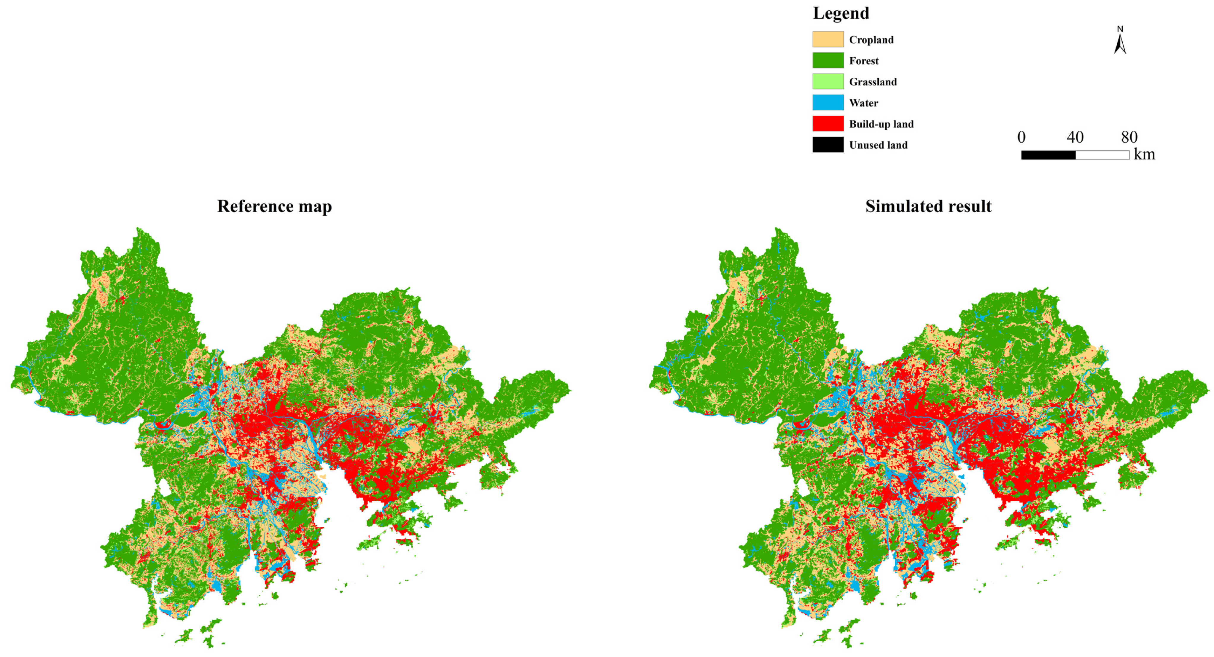
4.2. Simulation Validation

The CA–Markov model was validated over the period between 2005 and 2015. From the visualization map (Figure 6) and the corresponding quantitative evaluations (

Table 3. Accuracy assessment of land use simulation for 2015.

Land Use Type	PA (%)	UA (%)	OA (%)	Kappa	FOM (%)	T
Cropland	89.19	89.45	90.27	0.8495	89.14	587,686
Forest	90.41	98.11
Grassland	78.88	85.65
Water	99.95	81.30
Build-up land	88.79	73.14
Unused land	77.33	87.83

), it can be found that a relatively good simulation effect was obtained for 2015. Generally, the simulated result was basically in line with the reference map, whether from the whole land use pattern or spatial detail perspectives. The PA and UA of most land uses were over 85%, with the rest also over 70%, which suggested both the omission rate and commission rate were at a low level. In general, a high OA of 90.27%, Kappa of 0.8495, and FoM of 89.14% were obtained, with a low total error (T) of 587,686, which suggested the vast majority of geographical units and changes were correctly predicted. Therefore, the simulated result had a high consistency with the reference data [80,89].

More specifically, the prediction of forest land and cropland was accurate, according to the relatively high PAs and UAs, i.e., 90.41% and 89.19%, and 98.11% and 89.45%, which indicate less omissions and commissions. As part of the grassland and unused land were not successfully forecasted, the omission rate had a certain rise, leading to a decline in PAs, i.e., 78.88% and 77.33%, but these were still at an acceptable level for practical applications. For build-up land and water areas, due to the misprediction of some cells, the commission rate was relatively high, which leads to a certain decline in UAs, i.e., 73.14% and 81.30%.

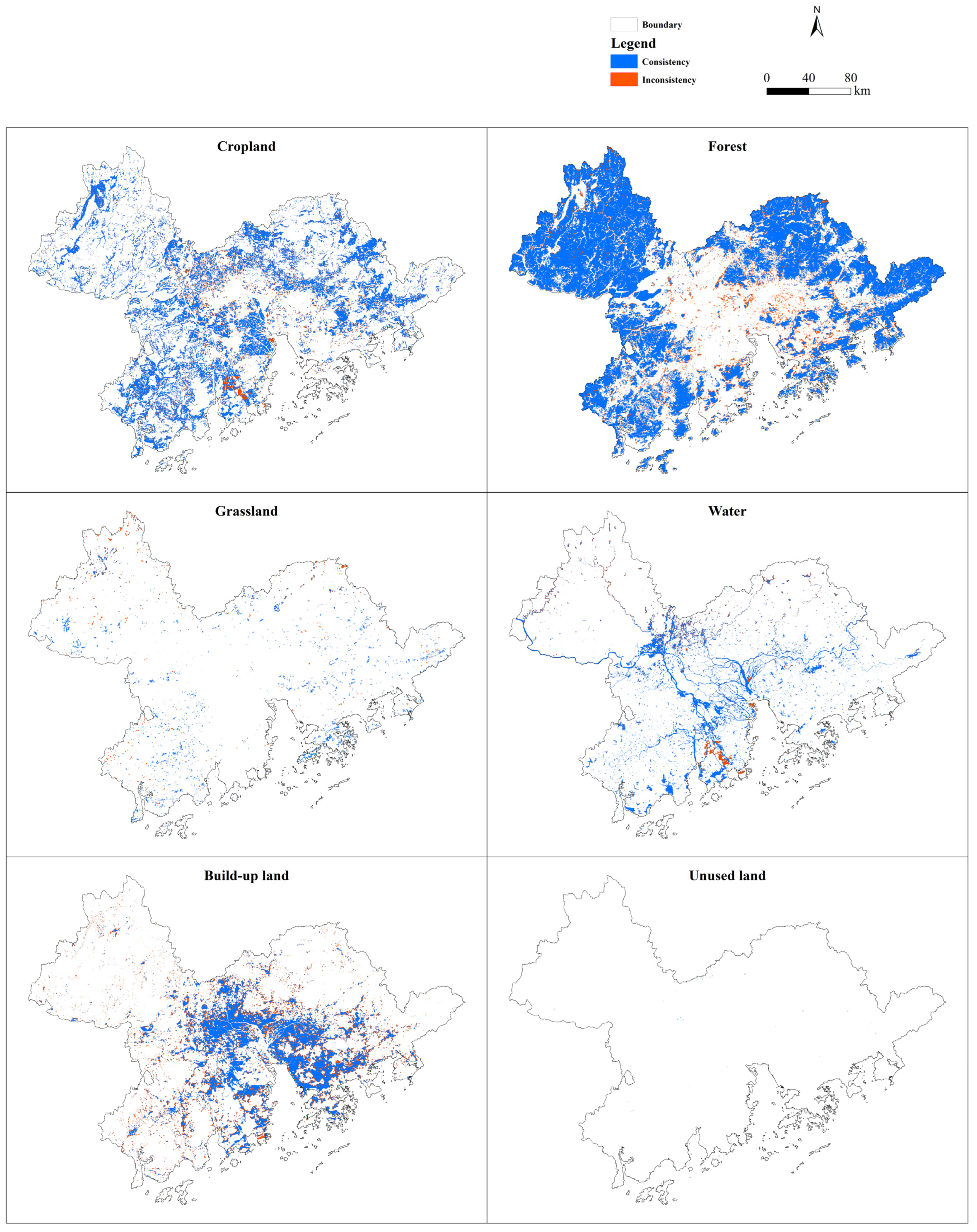
A spatial consistency map (Figure 7) for each land use was also given to indicate the position consistency between the simulated result and the reference map. In general, the simulation has a high consistency with the reference data for each use. Especially for forest land, the vast majority of geographical units were correctly forecasted. The simulation of grassland and unused land was also at an acceptable level, with relatively less inconsistences. For build-up land, the simulation was good in the central areas of the urban agglomeration, with inconsistences mainly scattered in the northwest and southwest of the GBA as well as the suburban areas. For cropland and water areas, the overall consistency was at a high level, with inconsistences mainly concentrated in the junction of Zhuhai and Zhongshan City, i.e., Doumen and Lianzhou Town. The reason may be that the main industry in these areas was aquaculture, with a large number of ponds embedded in arable land, which easily causes confusion between cropland and water areas.

Overall, the CA–Markov model has a good performance for land use simulation under complex circumstances and can be applied well to future multi-scenario simulations in the GBA.

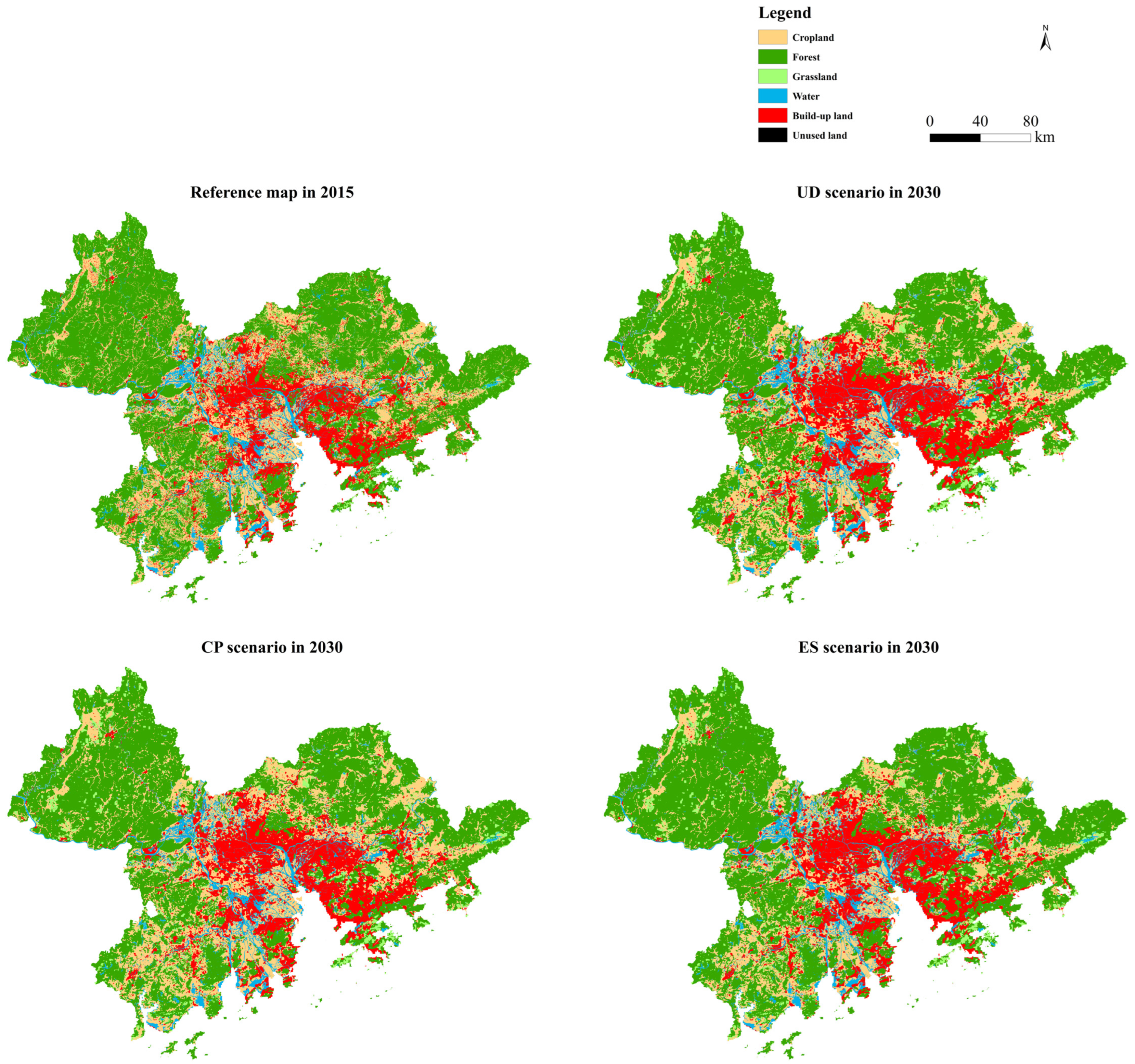
4.3. Multiple Scenario Simulations for Future Land Use Pattern

In order to explore the effects of different development modes and policies on LUCCs, land use patterns of the GBA in the short, medium, and long-term future, i.e., 2030, 2050, and 2070, were simulated with the validated CA–Markov model under UD, CP, and ES scenarios, respectively (Figure 8, Figure 9 and Figure 10). As illustrated in the figures, there were significant differences in the future land use structure between various scenarios, with the discrepancy magnified over time.

Specifically, it can be observed that urbanization will be the main melody for all three scenarios in the next decades, which is very obvious in the main body of the urban agglomeration, such as Shenzhen, Guangzhou, Foshan, Dongguan, and Zhongshan City. The urbanization expands from inside to outside and gradually connects into pieces, forming an increasing compact structure. Meanwhile, the marginal cities, such as Zhaoqing, Jiangmen, and Huizhou, also show a rapid growth on the original basis. In general, the newly added build-up areas are mainly distributed along both banks of the rivers, forming a typical belt-like expansion. However, the urbanization degree and LUCC pattern are quite different between various scenarios.

Under the UD scenario, the build-up land expands outwardly in a rapid and free manner, at the expenditure of any surrounding land use types. Accordingly, abundant cropland and forest areas are occupied, especially for the regions around cities, which leads to an immense reduction of arable land and woodland. By contrast, the forest loss is more significant, since most areas of the GBA are covered by woodland. This phenomenon will be more evident in 2050 and 2070 with the intensification of urbanization, which brings about a great challenge to the sustainability of the GBA.

Under the CP scenario, urbanization is obviously slowed down, with agricultural production and food security as primary objectives. The encroachment of cropland is significantly relieved in permanent farmland regions around cities, with cultivated land in other regions further enlarged under land reclamation activities, especially for the northwest and the south of the GBA, which is in accord with cropland protection policies and accounts for a certain increment of the total amount of cultivated land. Naturally, forest land has been the major consumptive land source of urbanization to meet the needs of urban development, with an increasing loss in the next decades.

Under the ES scenario, the ecological lands, in terms of forest, grassland, and water areas, are well protected without significant reduction, compared with that in 2015, which indicates an ecologically friendly development mode in the future. In the northwest and the northeast of the GBA, forest land and grassland have a certain increment, benefitting from ecological constructions and afforestation/greening projects. The urbanization becomes moderate under the restriction of ecological protection policies, with the occupation of ecological lands significantly reduced, which effectively relieves the contradictions between socio-economic development and ecological service. As the major expenditure of urbanization, cropland has an obvious reduction.

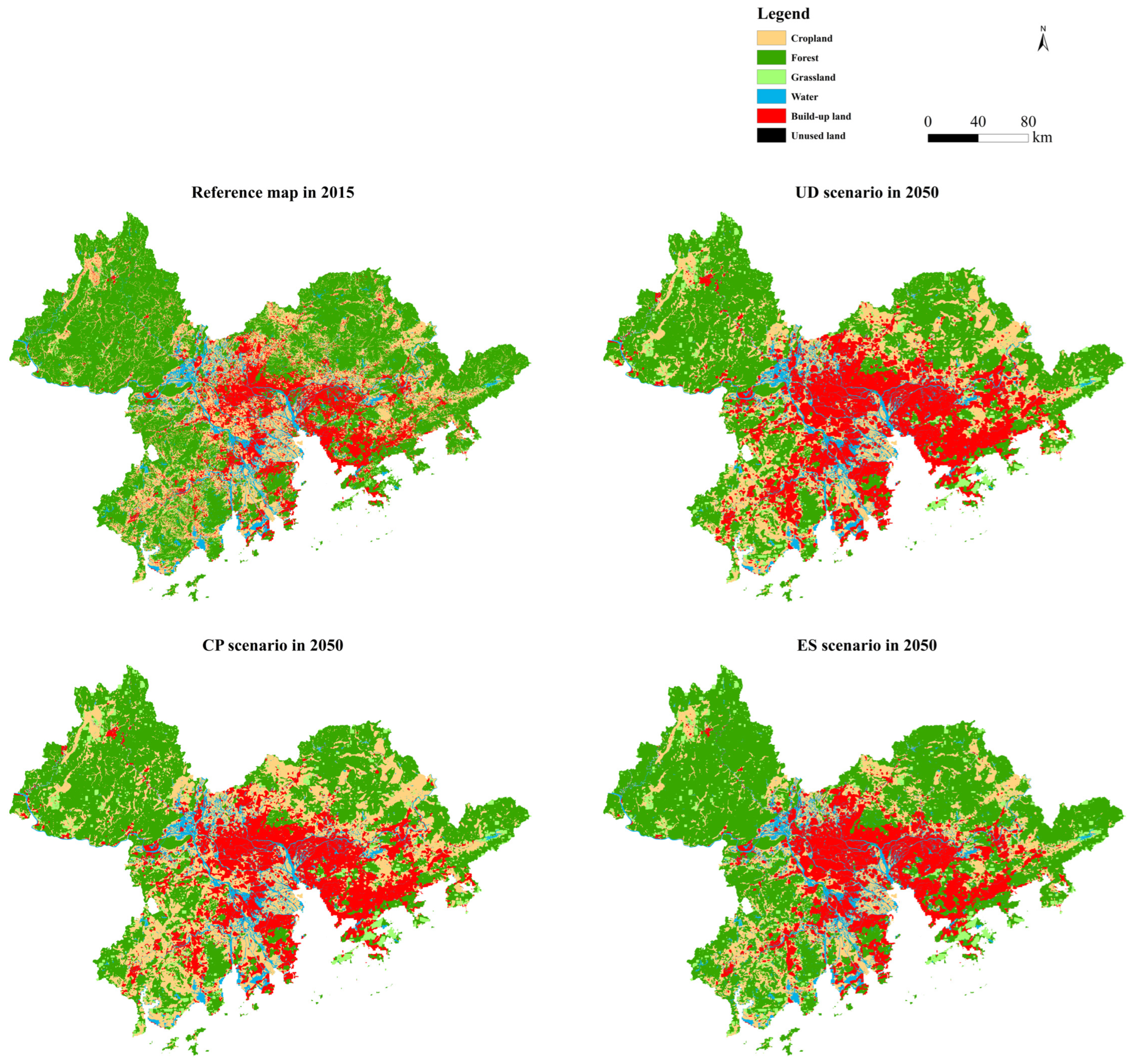
To gain further insight into the scenario differences, the land use details of three typical scenes in the medium term, i.e., 2050, are compared (Figure 11). It can be clearly observed that LUCCs differ a lot among the three scenarios. The UD scenario brings about a much more intensive urban sprawl under the principle of urban priority, with original discrete build-up areas connected into a piece and expanding outwardly in a rapid manner. The build-up land encroaches its surrounding land unscrupulously, which leads to large fragmentation to cropland and forest land. By comparison, the CP and ES scenarios restrict the free growth of build-up land to protect their preferred land use, with urbanization significantly relieved. More specifically, the CP scenario tries to avoid the expenditure of cropland, with forest land as the major land source of urbanization, as shown in the top left corner and middle lower part of Figure 11(a2), the left part of Figure 11(b2), and the lower right corner of Figure 11(c2). The EP scenario focuses on the protection of ecological lands, with urban sprawl mainly occurring in cropland regions. Consequently, it can be noted that the distribution of ecological lands, i.e., forest land, grassland, and water areas, have small changes compared with that in 2015.

4.4. Future Land System Dynamics under Multiple Scenarios

To better understand the influences of different scenario modes on the future land system evolution in the GBA, the differences in land allocation and dynamic patterns were further explored (

Table 4. Land allocation under multiple scenarios in 2030, 2050 and 2070 (km²).

Time	Scenario	Cropland	Forest	Grassland	Water	Build-Up Land	Unused Land
2030	UD	11,891.39	26,189.76	2123.79	3550.04	10,337.74	4.31
	CP	13,082.65	26,276.64	2132.02	3549.01	9052.39	4.32
	ES	10,856.46	28,659.44	2156.83	3572.24	8847.73	4.33
2050	UD	11,772.97	22,460.17	2311.55	3358.87	14,191.34	2.13
	CP	14,102.63	22,797.79	2342.44	3365.04	11,486.78	2.35
	ES	9669.38	27,859.89	2457.66	3525.93	10,581.83	2.34
2070	UD	11,967.37	18,154	2341.51	3130.48	18,502.74	0.93
	CP	15,377.63	18,661.33	2236	3032.34	14,788.58	1.15
	ES	8945.99	25,923.37	2558.55	3520.76	13,146.51	1.85

and Figure 12). It can be clearly observed that the future land dynamics will be quite different between the scenarios.

Under the UD scenario, the build-up area shows an excessive growth, profiting by priority policies, and significantly exceeds that under the other two scenarios. As shown in Table 4, The build-up area reaches 10,337.74 km² in 2030 and increases 2752.60 km² (36.29%) compared with that in 2015, with 1285.35 km² and 1490.01 km² more than the CP and EP scenarios. Additionally, it exceeds the planned area of 9938.20 km² in 2020, which demonstrates the effectiveness of this scenario for promoting urban development. Furthermore, urbanization will be accelerated during the periods between 2030 and 2050 and 2050 and 2070, with an increment of 3853.60 km² and 4311.40 km², respectively, leading to a gross gain of 10,917.60 km² (143.94%) during the period between 2015 and 2070. Accordingly, a large number of forests and croplands are occupied, with a gross loss of 11,187.09 km² (38.13%) and 500.39 km² (4.01%), which further exacerbates land contradictions and hinders regional sustainable development. It can be noted that forest land accounts for the main land source of urbanization and undergoes a continuous reduction. Water areas also decrease in the next decades, with a total loss of 389.93 km² (11.08%). Grassland continues an increasing trend as in 2005–2015, with an overall increment of 1165.32 km² (99.07%).

Under the CP scenario, cropland presents an obvious and constant growth, driven by cropland protection policies and land reclamation activities, forming a sharp contrast with that under the other two scenarios. As in Table 4, the gross area of cropland reaches 13,082.65 km² in 2030, with an increment of 1191.26 km² (10.02%), compared with that in 2015. It is up to 14,102.63 km² and 15,377.63 km² in 2050 and 2070, respectively, with a general gain of 2909.87 km² (23.34%) during the period between 2015 and 2070. On the other hand, build-up land still presents an increasing trend in the next decades, but with a much smaller magnitude, with a total increment of 7203.44 km² (94.97%). As a consequence, forest land constantly decreases, with a significant loss of 10,679.76 km² (36.40%). For water area and grassland, these types have similar dynamic trends as in the UD scenario, with a total loss of 488.07 km² (13.86%) and a total gain of 1059.81 km² (90.10%), respectively.

Under the ES scenario, ecological lands, including forest land, grassland, and water areas, show obvious advantages to ecological lands under the UD and CP scenarios, benefitting from ecology protection policies and afforestation/greening projects. As in Table 4, the build-up land increases at a mild rate, with a moderate increment of 5561.37 km² (73.32%) during the period between 2015 and 2070. Although forest land has certain reduction under urbanization, the magnitude is significantly reduced, with a gross loss of only 3417.72 km² (11.65%). The forest area is retained at 28,659.44 km² in 2030 and achieves the planned goal in 2020 of 28,405.62 km². For 2050 and 2070, it still remains at a high level of 27,859.89 km² and 25,923.37 km², without significant reduction, which suggests the effectiveness of this scenario in balancing socio-economic development and ecology security. As opposed to the other two scenarios, water resources are preserved under this scenario, and have a positive growth of 0.34 km². Grassland also presents a certain superiority, with a larger gross gain of 1382.36 km² (117.53%). Cropland inevitably decreases in a large magnitude as a consequence of urbanization, with a gross loss of 3521.77 km² (28.25%). However, the holding area of cropland in 2070 is 8945.99 km², far beyond the restricted basic farmland area of 7141.18 km² in 2020, which certainly guarantees regional agricultural production and food security [90,91,92].

4.5. The Effect of Land System Changes under Multiple Scenarios

In order to more deeply learn the differences and comparative advantages of various scenarios, in this section, the effect of land system changes concerning three major aspects, i.e., urban expansion, grain yield, and ecology quality, are comprehensively explored.

4.5.1. Urban Expansion Analysis

To better understand the urbanization characteristics of the GBA under various scenarios, three different quantitative metrics were utilized to indicate the internal pattern over two typical periods, i.e., 2030–2050 and 2050–2070 (Figure 13).

Generally, it can be observed that the UD scenario leads to much larger values of all three indices for most cities. More specifically, the developed cities, like Shenzhen, Zhuhai, and Hong Kong, which are affected by having a smaller jurisdiction and high-density construction, present a larger expansion intensity in both periods. Especially for Macao, it shows a significant expansion during the period between 2030 and 2050. However, restricted by the limited space, urbanization in Macao tends to be saturated in 2050–2070, with a very small expansion intensity. For the marginal cities with other major functions, like Zhaoqing and Huizhou, the broad jurisdiction makes urban sprawl inconspicuous and leads to a small expansion intensity.

On the other hand, Zhaoqing, Jiangmen, and Huizhou show a much larger expansion dynamicity compared with the developed cites, as a result of a smaller foundation area and high-intensity expansion. Meanwhile, it can be found that these three cities contribute most to the total urbanization of the GBA in both periods, accounting for more than half under the UD and CP scenarios during the period between 2030 and 2050 and under all three scenarios during the period between 2050 and 2070. Additionally, the contribution of Guangzhou and Foshan is also significant, especially under the ES scenario. In summary, the combination of further strengthening the core urban agglomeration and rapidly developing the marginal cities of the GBA is in accord with the general law of urbanization in China.

4.5.2. Grain Yield Estimation

To understand the impacts of different scenario modes on agricultural production, both the total grain yield of the GBA and the regional output of 11 internal cities under multiple scenarios in 2030, 2050, and 2070 were compared (

Table 5. Total grain yield under multiple scenarios in future years (ton).

Scenario	2030	2050	2070
Urban development	6,242,664.75	6,180,489	6,282,528
Cropland protection	6,868,076.25	7,403,555.25	8,072,893.5
Ecology security	5,699,326.5	5,076,109.5	4,696,324.5

and Figure 14).

It can be found that the CP scenario has an obvious superiority in grain yield in comparison to the other two scenarios, with an increasing total grain yield, which indicates its effectiveness in ensuring food security. The total grain yield of the GBA reaches 8,072,893.5 tons, with an increment of 17.54% during the period between 2030 and 2070, accounting for 1.21% of the national grain yield according to the reports in 2020.

The distribution of the grain yield among 11 internal cities is basically same for different scenarios and different years, with the main grain producing areas, such as Zhaoqing, Jiangmen, and Huizhou, having the largest contribution, followed by Guangzhou and Foshan. The sum of grain production in Zhaoqing, Jiangmen, and Huizhou accounts for more than 64% of the total output for all cases, with Jiangmen contributing the most. The developed cities, like Hong Kong, Macau, Shenzhen, Zhuhai, and Zhongshan, have a much lower grain yield, as they are highly industrialized with little room for agricultural development. On the other hand, it can be noted that under the CP scenario, the grain yield gradually increases in Zhaoqing, Jiangmen, and Huizhou, but is kept stable in the other cities.

4.5.3. Ecology Quality Evaluation

To compare the subsequent effects of LUCCs on the eco-environment under different scenarios, the total ecology quality index of the GBA in 2030, 2050, and 2070 was evaluated (

Table 6. Total ecology quality index under multiple scenarios in future years.

Scenario	2030	2050	2070
Urban development	5.3261	4.7496	4.2650
Cropland protection	5.3821	4.8486	4.3248
Ecology security	5.7017	5.5221	5.1725

), with regional ecology quality indices of 11 internal cities also provided (Figure 15).

Affected by urbanization, the total ecology quality of the GBA decreases for all three scenarios, with the UD scenario suffering from the fastest decline. Comparatively speaking, the ES scenario has the best ecology quality in all three years and shows a significant superiority to the other two scenarios. It maintains a basic stability for the eco-environment, with little degradation in the next decades. The total ecology quality of the GBA is retained at a high-level of 5.1725 in 2070 under the ES scenario, but it is reduced below 5 in 2050 under the UD and CP scenarios, with an obvious backwardness of 0.91 and 0.85 in 2070. The reason is that, driven by specific development orientations, i.e., the emphasis on cultivated land [93] and urban development priority [94], more and more ecological lands are encroached upon; woodland has the greatest ecological contribution, resulting in the continuous degradation of the eco-environment.

Similarly, the distribution of ecology quality is basically same for the different scenarios. With the passage of time, the gap between the ES and the other two scenarios becomes more and more obvious for most cities. Naturally, the marginal cities with high ecological land coverage, like Zhaoqing, Jiangmen, and Huizhou, have a better ecology quality. In contrast, the inner cities of the urban agglomeration, which are dominated by an impervious layer, have a much lower ecology quality, such as Zhuhai, Zhongshan, Shenzhen, Dongguan, and Macao. However, Hong Kong and Guangzhou are exceptions. Benefiting from a high vegetation coverage, these two cities maintain a high ecological value with the developed economy, whose development mode provides a good reference for others.

5. Discussion

5.1. Scenario Preference and Suitability for Regional Sustainability

The GBA is the fourth largest bay area in the world and is one of the regions with the highest openness degree and the strongest economic vitality in China. It has become a national planned strategic area in recent years, with grand development goals of not only being a world-class bay area and urban agglomeration but also being a high-quality life circle suitable for living, business, and tourism [46]. Due to the advantages of geographical location, many cities of the GBA have been at the forefront of reform and opening-up and have experienced unparallel development and urbanization, resulting in an increasingly prominent land use contradiction in this region [47,48]. Therefore, balancing socio-economic development, food security, and ecological needs has become a major concern to governments and planners. In order to promote land use optimization and formulate favorable policies to boost regional sustainability, multi-scenario simulations in the short, medium, and long-term future were comprehensively compared and analyzed in this study.

Under the UD scenario, the GBA will experience significant urbanization, with build-up land sustaining high-speed expansion, which greatly changes the original land use pattern. It provides a reasonable reference for possible locations and the upper-bound scale of urbanization in the next decades. However, under this scenario, urban expansion is excessive; the build-up area in 2030 far exceeds the planned area in 2020, and the build-up area in 2070 is almost twice of the planned area in 2020, which leads to a substantial reduction of forest land and cropland. Accordingly, along with rapid economic growth, the UD scenario will cause serious negative effects, such as agricultural production decline and ecology quality degradation. The woodland coverage will reduce from 54.24% in 2015 to 48.41%, 41.52%, and 33.56% in 2030, 2050, and 2070, respectively, which seriously degrades ecological service value in terms of water-and-soil conservation, regional climate regulation, as well as threats to species diversity in this region. All these violate the prerequisites of regional sustainability and the strategic positioning of high-quality development [50,53].

Under the CP scenario, urbanization will be slowed down to some degree, with the encroachment on arable land alleviated to a great extent. Meanwhile, with a supplement of new cultivated land under reclamation activities, the total amount of cropland exhibits an obvious growth in 2030, 2050, and 2070, which guarantees regional agricultural production and food security [95]. However, a large proportion of newly added cultivated land is located in mountainous areas, mainly concentrated in Zhaoqing, Jiangmen, and Huizhou, with complex terrain and relatively poor planting conditions in terms of soil nutrients, irrigation, and mechanization, which requires more investments to improve tillage quality to achieve comparable production in plain areas. Consequently, the overall agriculture input–output ratio will be pulled down to a certain degree. Furthermore, under the joint action of urbanization and land reclamation, extensive woodland will disappear, with a comparable ecological degradation to that under the UD scenario [96]. Generally, the land use pattern under this scenario has no protruding cost performance for regional high-quality development and is detrimental to the ecosystem [97].

Under the ES scenario, ecological lands, in terms of forest land, grassland, and water areas, will be well protected, without a significant reduction in the next decades compared with that in 2015. Regional ecology quality remains basically stable, which indicates an ecologically friendly development mode. On the other hand, urbanization has been restricted to a large extent to be more moderate, with a relatively proper incremental amount and a more reasonable/better-organized layout of built-up land [98]. The main roles of different functional areas, involving urban functional areas, ecological functional areas, and agricultural functional areas, can be better highlighted [99]. Meanwhile, although cropland suffers from a significant reduction under urbanization, the concentrated high-quality permanent farmland is properly protected to some extent, with the total cropland amount strictly controlled above the red line of cultivated land [100]. More specifically, the cropland area in 2070 is far beyond the planned minimum area of 7141.18 km² in 2020, which certainly ensures regional food security.

Overall, the land use pattern under the ES scenario seems more desirable and the corresponding development mode relives the intricate land contradictions between human and nature to a greater extent, which can be optimal for the future development of the GBA [101,102]. Under this scenario mode, a proper balance between socio-economy, agricultural production, and eco-environmental service will be built through land resource reallocation, which is conductive to promote the high-quality and green development of the GBA.

5.2. Future Land Use Optimization and Policy Formulation

According to the simulated results as shown in Figure 12, Figure 13, Figure 14 and Figure 15 and Table 4, Table 5 and Table 6, the ES scenario mode seems more suitable for the future development of the GBA. Accordingly, from a long-term perspective, land use management should stress the harmonization of socio-economic construction and eco-environmental security to form a benign development mode, through overall planning and comprehensive controls. Urban sprawl should be implemented at a moderate rate with a clear route and reasonable scope, without the extensive occupation of arable land and ecological lands. Additionally, land for resource-intensive and high-pollution industries should be sternly limited, with a preference for green and low-carbon industries, high-end manufacturing, and information-technology industries [50,53]. Moreover, regional ecology protection and restoration need to be further strengthened, with unnecessary construction land, cultivated land, and other lands returned to ecological lands.

On the other hand, regional decision-making and policy formulation should pay more attention to high-quality and green development, giving appropriate priority to ecology improvement. Socio-economic growth, ecological needs, and food security should be comprehensively taken into account for policy formulation [103,104,105]. For instance, the increment of build-up land should be limited within a rational range to leave enough ecological and agricultural space. It is imperative to take administrative measures to promote a regional industrial structure that is upgraded toward eco-friendly and deep-tech models, which has less land occupation, less use of natural resources, and less pollution [106,107]. Furthermore, a long-term ecological protection mechanism and a multi-level ecological protection system should be set up to build a high-quality life circle and boost the sustainable development of the GBA.

6. Conclusions

In this paper, the historical land system changes in the GBA from 2005 to 2015 were investigated; further, future land use patterns were simulated for 2030, 2050, and 2070 using a CA–Markov model under three tailored scenarios, i.e., UD, CP, and ES. The study found that excessive urbanization enlarged the urban space by 23.47% in the past decade, with substantial destruction of cropland, forest land, and water areas, leading to prominent land use contradictions. According to the simulated results, land use patterns will be significantly different in the next decades depending on which scenario mode is adopted, with disparate subsequent effects. Among the three scenarios, the ES scenario optimizes the balance between urban development and ecology protection, with promising perspectives for regional sustainable development. Thus, it is meaningful to restrict current excessive urban expansion, give appropriate priority to eco-environment improvement, and implement targeted land use optimization and positive policy formulation to promote future green development.

References

1. Liu, Y.; Xiao, X.; Li, J.; Wang, X.; Chen, B.; Sun, C.; Wang, C.; Tian, P.; Zhang, H. Tracking changes in coastal land cover in the Yellow Sea, East Asia, using Sentinel-1 and Sentinel-2 time-series images and Google Earth Engine. ISPRS J. Photogramm. Remote Sens. 2023, 196, 429–444. [Google Scholar] [CrossRef]
2. Chai, B.; Li, P. An ensemble method for monitoring land cover changes in urban areas using dense Landsat time series data. ISPRS J. Photogramm. Remote Sens. 2023, 195, 29–42. [Google Scholar] [CrossRef]
3. Calderón-Loor, M.; Hadjikakou, M.; Bryan, B.A. High-resolution wall-to-wall land-cover mapping and land change assessment for Australia from 1985 to 2015. Remote Sens. Environ. 2021, 252, 112148. [Google Scholar] [CrossRef]
4. Hu, M.; Ma, R.; Xiong, J.; Wang, M.; Cao, Z.; Xue, K. Eutrophication state in the Eastern China based on Landsat 35-year observations. Remote Sens. Environ. 2022, 277, 113057. [Google Scholar] [CrossRef]
5. Liu, W.; Li, H.; Xu, H.; Zhang, X.; Xie, Y. Spatiotemporal distribution and driving factors of regional green spaces during rapid urbanization in Nanjing metropolitan area, China. Ecol. Indic. 2023, 148, 110058. [Google Scholar] [CrossRef]
6. Cheng, Z.; Hu, X. The effects of urbanization and urban sprawl on CO2 emissions in China. Environ. Dev. Sustain. 2023, 25, 1792–1808. [Google Scholar] [CrossRef]
7. Li, L.; Zhan, W.; Ju, W.; Peñuelas, J.; Zhu, Z.; Peng, S.; Zhu, X.; Liu, Z.; Zhou, Y.; Li, J.; et al. Competition between biogeochemical drivers and land-cover changes determines urban greening or browning. Remote Sens. Environ. 2023, 287, 113481. [Google Scholar] [CrossRef]
8. Li, J.; Dong, S.; Li, Y.; Wang, Y.; Li, Z.; Li, F. Effects of land use change on ecosystem services in the China–Mongolia–Russia economic corridor. J. Clean. Prod. 2022, 360, 132175. [Google Scholar] [CrossRef]
9. Masum, K.M.; Islam, M.S.; Fahim, M.S.I.; Parvej, M.; Majeed, M.; Hasan, M.M.; Mansor, A. Temporal comparison of land-use changes and biodiversity in differential IUCN protected-area categories of Bangladesh in the context of co-management. Geol. Ecol. Landsc. 2023, 1–16. [Google Scholar] [CrossRef]
10. Shrestha, D.S.; Staab, B.D.; Duffield, J.A. Biofuel impact on food prices index and land use change. Biomass Bioenergy 2019, 124, 43–53. [Google Scholar] [CrossRef]
11. Zhai, H.; Lv, C.; Liu, W.; Yang, C.; Fan, D.; Wang, Z.; Guan, Q. Understanding spatio-temporal patterns of land use/land cover change under urbanization in Wuhan, China, 2000–2019. Remote Sens. 2021, 13, 3331. [Google Scholar] [CrossRef]
12. Liu, X.; Liang, X.; Li, X.; Xu, X.; Ou, J.; Chen, Y.; Li, S.; Wang, S.; Pei, F. A future land use simulation model (FLUS) for simulating multiple land use scenarios by coupling human and natural effects. Landsc. Urban Plan. 2017, 168, 94–116. [Google Scholar] [CrossRef]
13. Li, L.; Huang, X.; Yang, H. Scenario-based urban growth simulation by incorporating ecological-agricultural-urban suitability into a Future Land Use Simulation model. Cities 2023, 137, 104334. [Google Scholar] [CrossRef]
14. Song, X.P.; Hansen, M.C.; Stehman, S.V.; Potapov, P.V.; Tyukavina, A.; Vermote, E.F.; Townshend, J.R. Global land change from 1982 to 2016. Nature 2018, 560, 639–643. [Google Scholar] [CrossRef] [PubMed]
15. Van Dessel, W.; Van Rompaey, A.; Szilassi, P. Sensitivity analysis of logistic regression parameterization for land use and land cover probability estimation. Int. J. Geogr. Inf. Sci. 2011, 25, 489–508. [Google Scholar] [CrossRef]
16. Lin, Y.P.; Chu, H.J.; Wu, C.F.; Verburg, P.H. Predictive ability of logistic regression, auto-logistic regression and neural network models in empirical land-use change modeling—A case study. Int. J. Geogr. Inf. Sci. 2011, 25, 65–87. [Google Scholar] [CrossRef]
17. Shen, Q.; Chen, Q.; Tang, B.S.; Yeung, S.; Hu, Y.; Cheung, G. A system dynamics model for the sustainable land use planning and development. Habitat Int. 2009, 33, 15–25. [Google Scholar] [CrossRef]
18. Rasmussen, L.V.; Rasmussen, K.; Reenberg, A.; Proud, S. A system dynamics approach to land use changes in agro-pastoral systems on the desert margins of Sahel. Agric. Syst. 2012, 107, 56–64. [Google Scholar] [CrossRef]
19. Li, W.; Zhang, C. Application of transiograms to Markov chain simulation and spatial uncertainty assessment of land-cover classes. GISci. Remote Sens. 2005, 42, 297–319. [Google Scholar] [CrossRef]
20. Iacono, M.; Levinson, D.; El-Geneidy, A.; Wasfi, R. A Markov chain model of land use change. TeMA J. Land Use Mobil. Environ. 2015, 8, 263–276. [Google Scholar]
21. White, R.; Engelen, G. Cellular automata and fractal urban form: A cellular modelling approach to the evolution of urban land-use patterns. Environ. Plan. A 1993, 25, 1175–1199. [Google Scholar] [CrossRef]
22. de Almeida, C.M.; Batty, M.; Monteiro, A.M.V.; Câmara, G.; Soares-Filho, B.S.; Cerqueira, G.C.; Pennachin, C.L. Stochastic cellular automata modeling of urban land use dynamics: Empirical development and estimation. Comput. Environ. Urban Syst. 2003, 27, 481–509. [Google Scholar] [CrossRef]
23. Veldkamp, A.; Fresco, L.O. CLUE: A conceptual model to study the conversion of land use and its effects. Ecol. Model. 1996, 85, 253–270. [Google Scholar] [CrossRef]
24. Verburg, P.H.; Soepboer, W.; Veldkamp, A.; Limpiada, R.; Espaldon, V.; Mastura, S.S. Modeling the spatial dynamics of regional land use: The CLUE-S model. Environ. Manag. 2002, 30, 391–405. [Google Scholar] [CrossRef]
25. Matthews, R.B.; Gilbert, N.G.; Roach, A.; Polhill, J.G.; Gotts, N.M. Agent-based land-use models: A review of applications. Landsc. Ecol. 2007, 22, 1447–1459. [Google Scholar] [CrossRef]
26. Mena, C.F.; Walsh, S.J.; Frizzelle, B.G.; Xiaozheng, Y.; Malanson, G.P. Land use change on household farms in the Ecuadorian Amazon: Design and implementation of an agent-based model. Appl. Geogr. 2011, 31, 210–222. [Google Scholar] [CrossRef] [PubMed]
27. Arsanjani, J.J.; Helbich, M.; Kainz, W.; Boloorani, A.D. Integration of logistic regression, Markov chain and cellular automata models to simulate urban expansion. Int. J. Appl. Earth Obs. Geoinf. 2013, 21, 265–275. [Google Scholar] [CrossRef]
28. Cheng, L.; Sun, H.; Zhang, Y.; Zhen, S. Spatial structure optimization of mountainous abandoned mine land reuse based on system dynamics model and CLUE-S model. Int. J. Coal Sci. Technol. 2019, 6, 113–126. [Google Scholar] [CrossRef]
29. Halmy, M.W.A.; Gessler, P.E.; Hicke, J.A.; Salem, B.B. Land use/land cover change detection and prediction in the north-western coastal desert of Egypt using Markov-CA. Appl. Geogr. 2015, 63, 101–112. [Google Scholar] [CrossRef]
30. Wu, H.; Li, Z.; Clarke, K.C.; Shi, W.; Fang, L.; Lin, A.; Zhou, J. Examining the sensitivity of spatial scale in cellular automata Markov chain simulation of land use change. Int. J. Geogr. Inf. Sci. 2019, 33, 1040–1061. [Google Scholar] [CrossRef]
31. Lauf, S.; Haase, D.; Hostert, P.; Lakes, T.; Kleinschmit, B. Uncovering land-use dynamics driven by human decision-making–A combined model approach using cellular automata and system dynamics. Environ. Model. Softw. 2012, 27, 71–82. [Google Scholar] [CrossRef]
32. Liu, D.; Zheng, X.; Wang, H. Land-use simulation and decision-support system (LandSDS): Seamlessly integrating system dynamics, agent-based model, and cellular automata. Ecol. Model. 2020, 417, 108924. [Google Scholar] [CrossRef]
33. Verburg, P.H.; Overmars, K.P. Combining top-down and bottom-up dynamics in land use modeling: Exploring the future of abandoned farmlands in Europe with the Dyna-CLUE model. Landsc. Ecol. 2009, 24, 1167–1181. [Google Scholar] [CrossRef]
34. Sakayarote, K.; Shrestha, R.P. Simulating land use for protecting food crop areas in northeast Thailand using GIS and Dyna-CLUE. J. Geogr. Sci. 2019, 29, 803–817. [Google Scholar] [CrossRef]
35. Sang, L.; Zhang, C.; Yang, J.; Zhu, D.; Yun, W. Simulation of land use spatial pattern of towns and villages based on CA–Markov model. Math. Comput. Model. 2011, 54, 938–943. [Google Scholar] [CrossRef]
36. Munthali, M.G.; Mustak, S.; Adeola, A.; Botai, J.; Singh, S.K.; Davis, N. Modelling land use and land cover dynamics of Dedza district of Malawi using hybrid Cellular Automata and Markov model. Remote Sens. Appl. Soc. Environ. 2020, 17, 100276. [Google Scholar] [CrossRef]
37. Beroho, M.; Briak, H.; Cherif, E.K.; Boulahfa, I.; Ouallali, A.; Mrabet, R.; Kebede, F.; Bernardino, A.; Aboumaria, K. Future scenarios of land use/land cover (LULC) based on a CA-markov simulation model: Case of a mediterranean watershed in Morocco. Remote Sens. 2023, 15, 1162. [Google Scholar] [CrossRef]
38. He, J.; Huang, J.; Li, C. The evaluation for the impact of land use change on habitat quality: A joint contribution of cellular automata scenario simulation and habitat quality assessment model. Ecol. Model. 2017, 366, 58–67. [Google Scholar] [CrossRef]
39. Han, H.; Yang, C.; Song, J. Scenario simulation and the prediction of land use and land cover change in Beijing, China. Sustainability 2015, 7, 4260–4279. [Google Scholar] [CrossRef]
40. Zou, L.; Liu, Y.; Wang, J.; Yang, Y.; Wang, Y. Land use conflict identification and sustainable development scenario simulation on China’s southeast coast. J. Clean. Prod. 2019, 238, 117899. [Google Scholar] [CrossRef]
41. Yang, Y.; Bao, W.; Liu, Y. Scenario simulation of land system change in the Beijing-Tianjin-Hebei region. Land Use Policy 2020, 96, 104677. [Google Scholar] [CrossRef]
42. Li, H.; Wei, Y.D.; Ning, Y. Spatial and temporal evolution of urban systems in China during rapid urbanization. Sustainability 2016, 8, 651. [Google Scholar] [CrossRef]
43. Chaolin, G.U.; Liya, W.U.; Cook, I. Progress in research on Chinese urbanization. Front. Archit. Res. 2012, 1, 101–149. [Google Scholar] [CrossRef]
44. Zeng, P.; Wei, X.; Duan, Z. Coupling and coordination analysis in urban agglomerations of China: Urbanization and ecological security perspectives. J. Clean. Prod. 2022, 365, 132730. [Google Scholar] [CrossRef]
45. Huang, Y.; Li, L.; Yu, Y. Does urban cluster promote the increase of urban eco-efficiency? Evidence from Chinese cities. J. Clean. Prod. 2018, 197, 957–971. [Google Scholar] [CrossRef]
46. Hui, E.C.M.; Li, X.; Chen, T.; Lang, W. Deciphering the spatial structure of China’s megacity region: A new bay area-the Guangdong-Hong Kong-Macao Greater Bay Area in the making. Cities 2018, 105, 102168. [Google Scholar] [CrossRef]
47. Feng, R.; Wang, F.; Wang, K.; Xu, S. Quantifying influences of anthropogenic-natural factors on ecological land evolution in mega-urban agglomeration: A case study of Guangdong-Hong Kong-Macao greater Bay area. J. Clean. Prod. 2021, 283, 125304. [Google Scholar] [CrossRef]
48. Chen, Y.; Yan, H.; Yao, Y.; Zeng, C.; Gao, P.; Zhuang, L.; Fan, L.; Ye, D. Relationships of ozone formation sensitivity with precursors emissions, meteorology and land use types, in Guangdong-Hong Kong-Macao Greater Bay Area, China. J. Environ. Sci. 2020, 94, 1–13. [Google Scholar] [CrossRef] [PubMed]
49. Zhang, S.; Fang, C.; Kuang, W.; Sun, F. Comparison of changes in urban land use/cover and efficiency of megaregions in China from 1980 to 2015. Remote Sens. 2019, 11, 1834. [Google Scholar] [CrossRef]
50. Wu, Z.; Li, Z.; Zeng, H. Using remote sensing data to study the coupling relationship between urbanization and eco-environment change: A case study in the Guangdong-Hong Kong-Macao greater bay area. Sustainability 2020, 12, 7875. [Google Scholar] [CrossRef]
51. Wang, X.; Yan, F.; Su, F. Impacts of urbanization on the ecosystem services in the Guangdong-Hong Kong-Macao greater bay area, China. Remote Sens. 2020, 12, 3269. [Google Scholar] [CrossRef]
52. Yang, C.; Liu, H.; Li, Q.; Cui, A.; Xia, R.; Shi, T.; Zhang, J.; Gao, W.; Zhou, X.; Wu, G. Rapid urbanization induced extensive forest loss to urban land in the Guangdong-Hong Kong-Macao Greater Bay Area, China. Chin. Geogr. Sci. 2021, 31, 93–108. [Google Scholar] [CrossRef]
53. Chen, G.; Xie, J.; Li, W.; Li, X.; Chung, L.C.H.; Ren, C.; Liu, X. Future “local climate zone” spatial change simulation in Greater Bay Area under the shared socioeconomic pathways and ecological control line. Build. Environ. 2021, 203, 108077. [Google Scholar] [CrossRef]
54. Wang, R.Y.; Cai, H.; Chen, L.; Li, T. Spatiotemporal evolution and multi-scenario prediction of carbon storage in the GBA based on PLUS–InVEST models. Sustainability 2023, 15, 8421. [Google Scholar] [CrossRef]
55. Lv, C.; Lian, A.; Wang, Z.; Jia, T.; Sun, X.; Dong, R. A spatiotemporal pattern analysis of high-frequency land-use changes in the Guangdong–Hong Kong–Macao Greater Bay Area, from 1990 to 2018. Land 2022, 12, 102. [Google Scholar] [CrossRef]
56. Yu, W.; Zhou, W. Spatial pattern of urban change in two Chinese megaregions: Contrasting responses to national policy and economic mode. Sci. Total Environ. 2018, 634, 1362–1371. [Google Scholar] [CrossRef]
57. Bai, Y.; Wong, C.P.; Jiang, B.; Hughes, A.C.; Wang, M.; Wang, Q. Developing China’s Ecological Redline Policy using ecosystem services assessments for land use planning. Nat. Commun. 2018, 9, 3034. [Google Scholar] [CrossRef]
58. Leta, M.K.; Demissie, T.A.; Tränckner, J. Modeling and prediction of land use land cover change dynamics based on land change modeler (Lcm) in nashe watershed, upper blue nile basin, Ethiopia. Sustainability 2021, 13, 3740. [Google Scholar] [CrossRef]
59. Bryan, B.A.; Nolan, M.; McKellar, L.; Connor, J.D.; Newth, D.; Harwood, T.; King, D.; Navarro, J.; Cai, Y.; Gao, L.; et al. Land-use and sustainability under intersecting global change and domestic policy scenarios: Trajectories for Australia to 2050. Glob. Environ. Chang. 2016, 38, 130–152. [Google Scholar] [CrossRef]
60. Gerland, P.; Raftery, A.E.; Ševčíková, H.; Li, N.; Gu, D.; Spoorenberg, T.; Alkema, L.; Fosdick, B.K.; Chunn, J.; Lalic, N.; et al. World population stabilization unlikely this century. Science 2014, 346, 234–237. [Google Scholar] [CrossRef]
61. Popp, A.; Calvin, K.; Fujimori, S.; Havlik, P.; Humpenöder, F.; Stehfest, E.; Bodirsky, B.L.; Dietrich, J.P.; Doelmann, J.C.; Gusti, M.; et al. Land-use futures in the shared socio-economic pathways. Glob. Environ. Chang. 2017, 42, 331–345. [Google Scholar] [CrossRef]
62. Bryan, B.A.; Meyer, W.S.; Campbell, C.A.; Harris, G.P.; Lefroy, T.; Lyle, G.; Martin, P.; McLean, J.; Montagu, K.; Rickards, L.A.; et al. The second industrial transformation of Australian landscapes. Curr. Opin. Environ. Sustain. 2013, 5, 278–287. [Google Scholar] [CrossRef]
63. Newell, R.G.; Pizer, W.A.; Raimi, D. Carbon market lessons and global policy outlook. Science 2014, 343, 1316–1317. [Google Scholar] [CrossRef] [PubMed]
64. Dang, V.Q.; Kwan, F.; Lam, A.I. Guangdong–Hong Kong–Macao Greater Bay Area (GBA): Economic progress, diversification, and convergence. J. Asia Pac. Econ. 2023, 1–31. [Google Scholar] [CrossRef]
65. Wang, Y.; Han, Z.; Gao, R. Changes of extreme high temperature and heavy precipitation in the Guangdong-Hong Kong-Macao Greater Bay Area. Geomat. Nat. Hazards Risk 2021, 12, 1101–1126. [Google Scholar] [CrossRef]
66. Wu, J.; Zhang, D.; Wang, H.; Li, X. What is the future for production-living-ecological spaces in the Greater Bay Area? A multi-scenario perspective based on DEE. Ecol. Indic. 2021, 131, 108171. [Google Scholar] [CrossRef]
67. Yok-shiu, F.L. Tackling cross-border environmental problems in Hong Kong: Initial responses and institutional constraints. China Q. 2002, 172, 986–1009. [Google Scholar]
68. Hou, X.; Chan, C.K.; Dong, G.H.; Yim, S.H. Impacts of transboundary air pollution and local emissions on PM2. 5 pollution in the Pearl River Delta region of China and the public health, and the policy implications. Environ. Res. Lett. 2019, 14, 034005. [Google Scholar] [CrossRef]
69. Liu, J.; Kuang, W.; Zhang, Z.; Xu, X.; Qin, Y.; Ning, J.; Zhou, W.; Zhang, W.; Zhang, S.; Li, R.; et al. Spatiotemporal characteristics, patterns, and causes of land-use changes in China since the late 1980s. J. Geogr. Sci. 2014, 24, 195–210. [Google Scholar] [CrossRef]
70. Kuang, W.; Liu, J.; Dong, J.; Chi, W.; Zhang, C. The rapid and massive urban and industrial land expansions in China between 1990 and 2010: A CLUD-based analysis of their trajectories, patterns, and drivers. Landsc. Urban Plan. 2016, 145, 21–33. [Google Scholar] [CrossRef]
71. Guan, D.; Li, H.; Inohae, T.; Su, W.; Nagaie, T.; Hokao, K. Modeling urban land use change by the integration of cellular automaton and Markov model. Ecol. Model. 2011, 222, 3761–3772. [Google Scholar] [CrossRef]
72. Keshtkar, H.; Voigt, W. A spatiotemporal analysis of landscape change using an integrated Markov chain and cellular automata models. Model. Earth Syst. Environ. 2016, 2, 1–13. [Google Scholar] [CrossRef]
73. Zhang, Y.; Li, X.; Liu, X.; Qiao, J. Self-modifying CA model using dual ensemble Kalman filter for simulating urban land-use changes. Int. J. Geogr. Inf. Sci. 2015, 29, 1612–1631. [Google Scholar] [CrossRef]
74. Wang, S.Q.; Zheng, X.Q.; Zang, X.B. Accuracy assessments of land use change simulation based on Markov-cellular automata model. Procedia Environ. Sci. 2012, 13, 1238–1245. [Google Scholar] [CrossRef]
75. Fu, X.; Wang, X.; Yang, Y.J. Deriving suitability factors for CA-Markov land use simulation model based on local historical data. J. Environ. Manag. 2018, 206, 10–19. [Google Scholar] [CrossRef] [PubMed]
76. Subedi, P.; Subedi, K.; Thapa, B. Application of a hybrid cellular automaton–Markov (CA-Markov) model in land-use change prediction: A case study of Saddle Creek Drainage Basin, Florida. Appl. Ecol. Environ. Sci. 2013, 1, 126–132. [Google Scholar] [CrossRef]
77. López, E.; Bocco, G.; Mendoza, M.; Duhau, E. Predicting land-cover and land-use change in the urban fringe: A case in Morelia city, Mexico. Landsc. Urban Plan. 2001, 55, 271–285. [Google Scholar] [CrossRef]
78. Singh, S.K.; Mustak, S.; Srivastava, P.K.; Szabó, S.; Islam, T. Predicting spatial and decadal LULC changes through cellular automata Markov chain models using earth observation datasets and geo-information. Environ. Process. 2015, 2, 61–78. [Google Scholar] [CrossRef]
79. Aburas, M.M.; Ho, Y.M.; Ramli, M.F.; Ash’aari, Z.H. Improving the capability of an integrated CA-Markov model to simulate spatio-temporal urban growth trends using an Analytical Hierarchy Process and Frequency Ratio. Int. J. Appl. Earth Obs. Geoinf. 2017, 59, 65–78. [Google Scholar] [CrossRef]
80. Zhou, L.; Dang, X.; Sun, Q.; Wang, S. Multi-scenario simulation of urban land change in Shanghai by random forest and CA-Markov model. Sustain. Cities Soc. 2020, 55, 102045. [Google Scholar] [CrossRef]
81. Hamad, R.; Balzter, H.; Kolo, K. Predicting land use/land cover changes using a CA-Markov model under two different scenarios. Sustainability 2018, 10, 3421. [Google Scholar] [CrossRef]
82. Pontius, R.G., Jr.; Peethambaram, S.; Castella, J.C. Comparison of three maps at multiple resolutions: A case study of land change simulation in Cho Don District, Vietnam. Ann. Assoc. Am. Geogr. 2011, 101, 45–62. [Google Scholar] [CrossRef]
83. Liu, Y.; Luo, T.; Liu, Z.; Kong, X.; Li, J.; Tan, R. A comparative analysis of urban and rural construction land use change and driving forces: Implications for urban–rural coordination development in Wuhan, Central China. Habitat Int. 2015, 47, 113–125. [Google Scholar] [CrossRef]
84. Cuba, N. Research note: Sankey diagrams for visualizing land cover dynamics. Landsc. Urban Plan. 2015, 139, 163–167. [Google Scholar] [CrossRef]
85. Al-Sharif, A.A.; Pradhan, B.; Shafri, H.Z.M.; Mansor, S. Quantitative analysis of urban sprawl in Tripoli using Pearson’s Chi-Square statistics and urban expansion intensity index. IOP Conf. Ser. Earth Environ. Sci. 2014, 20, 012006. [Google Scholar] [CrossRef]
86. Hu, Z.L.; Du, P.J.; Guo, D.Z. Analysis of urban expansion and driving forces in Xuzhou city based on remote sensing. J. China Univ. Min. Technol. 2007, 17, 267–271. [Google Scholar] [CrossRef]
87. Yuan, S.F.; Tang, Y.Y.; Shen, T.C.N. Spatiotemporal change of land-use transformation and its eco-environmental response: A case of 127 counties in Yangtze River Economic Belt. Econ. Geogr. 2019, 39, 174–181. [Google Scholar]
88. Gong, Y.N.; Han, S.C.; Shi, X.B.; Tang, X.M. The spatiotemporal evolution and ecological environmental effects of the transformation of land use in Guangdong Province’s three living spaces. Res. Soil Water Conserv. 2020, 27, 203–209. [Google Scholar]
89. García, A.M.; Santé, I.; Boullón, M.; Crecente, R. A comparative analysis of cellular automata models for simulation of small urban areas in Galicia, NW Spain. Comput. Environ. Urban Syst. 2012, 36, 291–301. [Google Scholar] [CrossRef]
90. Gardi, C.; Panagos, P.; Van Liedekerke, M.; Bosco, C.; De Brogniez, D. Land take and food security: Assessment of land take on the agricultural production in Europe. J. Environ. Plan. Manag. 2015, 58, 898–912. [Google Scholar] [CrossRef]
91. Zabel, F.; Delzeit, R.; Schneider, J.M.; Seppelt, R.; Mauser, W.; Václavík, T. Global impacts of future cropland expansion and intensification on agricultural markets and biodiversity. Nat. Commun. 2019, 10, 2844. [Google Scholar] [CrossRef] [PubMed]
92. He, C.; Liu, Z.; Xu, M.; Ma, Q.; Dou, Y. Urban expansion brought stress to food security in China: Evidence from decreased cropland net primary productivity. Sci. Total Environ. 2017, 576, 660–670. [Google Scholar] [CrossRef] [PubMed]
93. Huo, J.; Shi, Z.; Zhu, W.; Xue, H.; Chen, X. A multi-scenario simulation and optimization of land use with a Markov–FLUS coupling model: A case study in Xiong’an New Area, China. Sustainability 2022, 14, 2425. [Google Scholar] [CrossRef]
94. Lin, X.; Fu, H. Multi-scenario simulation analysis of cultivated land based on PLUS model—A case study of Haikou, China. Front. Ecol. Evol. 2023, 11, 1197419. [Google Scholar] [CrossRef]
95. Li, Y.; Liu, Z.; Li, S.; Li, X. Multi-scenario simulation analysis of land use and carbon storage changes in changchun city based on FLUS and InVEST model. Land 2022, 11, 647. [Google Scholar] [CrossRef]
96. Chen, Z.; Huang, M.; Zhu, D.; Altan, O. Integrating remote sensing and a markov-FLUS model to simulate future land use changes in Hokkaido, Japan. Remote Sens. 2021, 13, 2621. [Google Scholar] [CrossRef]
97. Bao, W.; Yang, Y.; Zou, L. How to reconcile land use conflicts in mega urban agglomeration? A scenario-based study in the Beijing-Tianjin-Hebei region, China. J. Environ. Manag. 2021, 296, 113168. [Google Scholar] [CrossRef] [PubMed]
98. Yin, H.; Kong, F.; Hu, Y.; James, P.; Xu, F.; Yu, L. Assessing growth scenarios for their landscape ecological security impact using the SLEUTH urban growth model. J. Urban Plan. Dev. 2016, 142, 05015006. [Google Scholar] [CrossRef]
99. Li, L.; Huang, X.; Wu, D.; Yang, H. Construction of ecological security pattern adapting to future land use change in Pearl River Delta, China. Appl. Geogr. 2023, 154, 102946. [Google Scholar] [CrossRef]
100. Hoque, M.Z.; Cui, S.; Islam, I.; Xu, L.; Tang, J. Future impact of land use/land cover changes on ecosystem services in the lower meghna river estuary, Bangladesh. Sustainability 2020, 12, 2112. [Google Scholar] [CrossRef]
101. Wang, C.; Yu, C.; Chen, T.; Feng, Z.; Hu, Y.; Wu, K. Can the establishment of ecological security patterns improve ecological protection? An example of Nanchang, China. Sci. Total Environ. 2020, 740, 140051. [Google Scholar] [CrossRef] [PubMed]
102. Li, Y.; Liu, W.; Feng, Q.; Zhu, M.; Yang, L.; Zhang, J.; Yin, X. The role of land use change in affecting ecosystem services and the ecological security pattern of the Hexi Regions, Northwest China. Sci. Total Environ. 2023, 855, 158940. [Google Scholar] [CrossRef] [PubMed]
103. Wang, J.; Chen, T. A Multi-Scenario Land Expansion Simulation Method from Ecosystem Services Perspective of Coastal Urban Agglomeration: A Case Study of GHM-GBA, China. Land 2022, 11, 1934. [Google Scholar] [CrossRef]
104. Wang, Y.; Yao, Y.; Chen, S.; Ni, Z.; Xia, B. Spatiotemporal evolution of urban development and surface urban heat island in Guangdong-Hong Kong-Macau greater bay area of China from 2013 to 2019. Resour. Conserv. Recycl. 2022, 179, 106063. [Google Scholar] [CrossRef]
105. Yang, C.; Guo, W.; Zhang, C.; Cui, A.; Li, X.; Zhao, T.; Liu, H.; Shi, T.; Xu, G.; Fang, X.; et al. Characteristics and trends of hillside urbanization in China from 2007 to 2017. Habitat Int. 2022, 120, 102502. [Google Scholar] [CrossRef]
106. Kruachottikul, P.; Dumrongvute, P.; Tea-makorn, P.; Kittikowit, S.; Amrapala, A. New product development process and case studies for deep-tech academic research to commercialization. J. Innov. Entrep. 2023, 12, 48. [Google Scholar] [CrossRef]
107. De la Tour, A.; Soussan, P.; Harlé, N.; Chevalier, R.; Duportet, X. From Tech to Deep Tech; Boston Consulting Group: Boston, MA, USA, 2017; p. 52. [Google Scholar]
Figure 1. The location of the Guangdong–Hong Kong–Macao Greater Bay Area.
Remotesensing 16 01512 g001
Figure 2. Visualization of various driving factors.
Remotesensing 16 01512 g002
Figure 3. Overall route of the CA–Markov model for land use simulation.
Remotesensing 16 01512 g003
Figure 4. Land use pattern of the GBA in the past decade: 2005, 2010, and 2015.
Remotesensing 16 01512 g004
Figure 5. Sankey diagram for land use conversion from 2005 to 2015.
Remotesensing 16 01512 g005
Figure 6. Land use simulation for 2015 in the GBA.
Remotesensing 16 01512 g006
Figure 7. The spatial consistency map for each land use in 2015.
Remotesensing 16 01512 g007
Figure 8. Multi-scenario simulation for 2030.
Remotesensing 16 01512 g008
Figure 9. Multi-scenario simulation for 2050.
Remotesensing 16 01512 g009
Figure 10. Multi-scenario simulation for 2070.
Remotesensing 16 01512 g010
Figure 11. Spatial details of three typical scenes under various scenarios in 2050: (ac) denote reference map in 2015; (a1c1) denote simulated results under the UD scenario; (a2c2) denote simulated results under the CP scenario; and (a3c3) denote simulated results under the ES scenario.
Remotesensing 16 01512 g011
Figure 12. Land use dynamics in the period of 2015–2030, 2030–2050, and 2050–2070 under multiple scenarios.
Remotesensing 16 01512 g012
Figure 13. Urban expansion of different cities in the GBA under multiple scenarios in the next decades.
Remotesensing 16 01512 g013
Figure 14. Grain yield of different cities in the GBA under multiple scenarios in future years.
Remotesensing 16 01512 g014
Figure 15. Ecology quality index of different cities in the GBA under multiple scenarios in future years.
Remotesensing 16 01512 g015