Article

Regional Real-Time between-Satellite Single-Differenced Ionospheric Model Establishing by Multi-GNSS Single-Frequency Observations: Performance Evaluation and PPP Augmentation

1
College of Geoscience and Surveying Engineering, China University of Mining and Technology-Beijing, Beijing 100083, China
2
Shanghai Astronomical Observatory, Chinese Academy of Sciences, Shanghai 200030, China
3
School of Astronomy and Space Science, University of Chinese Academy of Sciences, Beijing 100049, China
4
School of Environment Science and Spatial Informatics, China University of Mining and Technology, Xuzhou 221116, China
5
Chinese Academy of Surveying & Mapping, Beijing 100036, China
*
Author to whom correspondence should be addressed.
Remote Sens. 2024, 16(9), 1511; https://doi.org/10.3390/rs16091511
Submission received: 14 March 2024 / Revised: 11 April 2024 / Accepted: 22 April 2024 / Published: 25 April 2024

Abstract

:
The multi-global navigation satellite system (GNSS) undifferenced and uncombined precise point positioning (UU-PPP), as a high-precision ionospheric observables extraction technology superior to the traditional carrier-to-code leveling (CCL) method, has received increasing attention. In previous research, only dual-frequency (DF) or multi-frequency (MF) observations are used to extract slant ionospheric delay with the UU-PPP. To reduce the cost of ionospheric modeling, the feasibility of extracting ionospheric observables from the multi-GNSS single-frequency (SF) UU-PPP was investigated in this study. Meanwhile, the between-satellite single-differenced (SD) method was applied to remove the effects of the receiver differential code bias (DCB) with short-term time-varying characteristics in regional ionospheric modeling. In the assessment of the regional real-time (RT) between-satellite SD ionospheric model, the internal accord accuracy of the SD ionospheric delay can be better than 0.5 TECU, and its external accord accuracy within 1.0 TECU is significantly superior to three global RT ionospheric models. With the introduction of the proposed SD ionospheric model into the multi-GNSS kinematic RT SF-PPP, the initialization speed of vertical positioning errors can be improved by 21.3% in comparison with the GRAPHIC (GRoup And PHase Ionospheric Correction) SF-PPP model. After reinitialization, both horizontal and vertical positioning errors of the SD ionospheric constrained (IC) SF-PPP can be maintained within 0.2 m. This proves that the proposed SDIC SF-PPP model can enhance the continuity and stability of kinematic positioning in the case of some GNSS signals missing or blocked. Compared with the GRAPHIC SF-PPP, the horizontal positioning accuracy of the SDIC SF-PPP in kinematic mode can be improved by 37.9%, but its vertical positioning accuracy may be decreased. Overall, the 3D positioning accuracy of the SD ionospheric-constrained RT SF-PPP can be better than 0.3 m.

1. Introduction

As one of the most serious interference factors in radio signals, the ionospheric delay has a significant negative impact on the global navigation satellite system (GNSS) data processing, especially in the precise point positioning (PPP) domain [1,2]. If GNSS users can afford expensive dual-frequency (DF) receivers, ionospheric errors can be eliminated by over 99% by forming a DF ionosphere-free (IF) combination model. However, the majority of smart devices, such as mobile phones and wristwatches, can only be equipped with single-frequency (SF) GNSS chipsets, making it impossible to adopt the IF model to weaken ionospheric errors [3,4]. To achieve low-cost and high-precision SF positioning, many kinds of broadcast or post-processing ionospheric models have been proposed so far. Although the GPS Klobuchar model, BeiDou global broadcast ionospheric delay correction model (BDGIM), and Galileo NeQuick model can be applied to real-time (RT) SF positioning, their ionospheric correction capabilities are limited and no more than 80% [5,6,7,8]. The post-processed global ionospheric map (GIM), as one of the most accurate ionospheric models, can provide correction accuracy within two total electron content units (TECU), but it cannot support RT positioning [9]. With the development of the Real-Time Working Group (RTWG) of the International GNSS Service (IGS), an RT-GIM has been provided by some IGS real-time ionosphere centers. The accuracy of RT-GIM is slightly lower than that of post-processed GIM and can reach around 3 TECU [10]. Due to the limited accuracy of the current RT ionospheric models, it is necessary to establish an RT ionospheric model with cm-level accuracy using regional reference networks to improve the performance of RT SF-PPP.
On the premise of not changing the number of regional monitoring stations, there are two main factors that affect the quality of ionospheric modeling. One is the extraction accuracy of ionospheric delay observables, and another is the calculation accuracy of the differential code bias (DCB) for satellite and receiver. The traditional carrier-to-code leveling (CCL) method has been widely used in ionospheric modeling due to its simple structure and high computational efficiency. Nevertheless, the accuracy of ionospheric delay extracted by this method is limited and is susceptible to adverse effects of multipath errors and code noises [11,12]. Thanks to the preservation of ionospheric parameters in the undifferenced and uncombined (UU) PPP, a novel method based on carrier phase observations for extracting ionospheric delays has been proposed [13]. Compared with the CCL method, the accuracy of slant ionospheric delays derived from the UU-PPP can be improved at least three times to 0.1 TECU. As expected, the modeling accuracy of regional ionospheric vertical total electron content (VTEC) using the UU-PPP method is better than that using the CCL method [14].
Due to the presence of hardware bias in retrieved ionospheric observables, it is necessary to simultaneously estimate both satellite and receiver DCB parameters when modeling ionospheric VTEC. The satellite DCB has great long-term stability, so its solution accuracy is high and reliable [15]. Unfortunately, the receiver DCB is easily influenced by various factors, such as ambient temperature and hardware alternation. Thus, its apparent short-term time-varying characteristics can be observed [16,17]. If the receiver DCB as an additional parameter was estimated in UU-PPP, although pure slant ionospheric delays can be obtained [18], the increase in estimated parameters reduces the strength and computational efficiency of the UU-PPP model. Meanwhile, the high-frequency parameterization of receiver DCB will inevitably increase the burden and cost of data transmission, making it difficult to apply to RT ionospheric modeling based on dense reference networks.
To completely remove the adverse effects of receiver DCB and meet the requirements of time-critical in RT ionospheric modeling, a regional RT ionospheric model was established using the classical between-satellite single-differenced (SD) method [19]. Since the receiver DCB can be precisely eliminated and high-precision ionospheric observables are derived from the UU-PPP, the accuracy of the proposed RT ionospheric model is significantly better than that of the post-processing GIM model. However, the implementation of this high-quality ionospheric model must be based on the use of GNSS DF observations. Thus, the hardware cost of the modeling system is very expensive. Considering that the multi-GNSS SF UU-PPP has the ability to achieve cm-level accuracy at present [20,21], in our study, the possibility of modeling a regional RT between-satellite SD ionospheric model based on SF observations was explored and verified. This is extremely important for low-cost SF positioning users. Different from the literature [19] only using GPS and Galileo observations, the BDS-3 observations were introduced into multi-GNSS processing in this contribution, which can improve the performance of the regional RT between-satellite SD ionospheric model by increasing the spatial resolution of the ionosphere pierce point (IPP). In summary, this contribution is to attempt to reduce the hardware cost of ionospheric modeling and provide an effective solution for building high-precision regional ionospheric models only using affordable SF devices or chips in the future.
The writing structure of this paper is as follows: first, the extraction method of slant ionospheric observables using multi-GNSS SF UU-PPP technology, modeling algorithm of the regional RT between-satellite SD ionospheric delay, and ionospheric-constrained multi-GNSS SF-PPP model are introduced in detail. Then, the experimental data for the European region and processing strategies in both ionospheric modeling and positioning domains are presented. After evaluating the performance of the regional RT between-satellite SD ionospheric model, its contribution to the multi-GNSS RT SF-PPP is analyzed. In the final section, some new findings and conclusions are summarized.

2. Methods

Thanks to the advantages of abundant satellite resources and high sampling rates for the GNSS technology, ionospheric observables with low-cost and high spatial-temporal resolution can be obtained from the multi-GNSS SF UU-PPP. The modeling method of the regional RT between-satellite SD ionospheric delay is described in this section. To optimize the RT kinematic positioning performance of SF users, a novel multi-GNSS RT SF-PPP model based on the SD ionospheric constraints is proposed.

2.1. Extraction of Slant Ionospheric Observables from Single-Frequency UU-PPP

The GNSS raw code P r , 1 s and phase L r , 1 s observations at the first frequency can be expressed as [14]
{ P r , 1 s = ρ r s + c ( d t r d t s ) + T r s + I 1 s + B r , 1 B 1 s + ε p 1 L r , 1 s = ρ r s + c ( d t r d t s ) + T r s I 1 s + ω 1 s + N r , 1 s + b r , 1 b 1 s + ε L 1
where the superscript s and subscript r denote the satellite and GNSS receiver, respectively. ρ k s is the calculated distance between the satellite and the GNSS receiver. c denotes the speed of light. d t r and d t s denote the clock errors of the satellite and GNSS receiver, respectively. T r s denotes the slant tropospheric delay errors, I 1 s denotes the slant ionospheric errors. ω 1 s denotes the carrier phase wind-up errors. N r , 1 s denotes the integer ambiguity of carrier phase. B r , 1 denotes the code hardware delays of the GNSS receiver, and B 1 s denotes the code hardware delays of the satellite. b r , 1 denotes the phase hardware delays of the GNSS receiver, and b 1 s denotes the phase hardware delays of the satellite. ε p 1 and ε L 1 denote the code and phase observation noises, respectively.
In RT SF-PPP, the satellite and receiver clock errors need to be corrected using code hardware delays because the RT precise satellite clocks provided by the IGS real-time service (RTS) are obtained from the DF IF observations. Hence, the reparametrized clock errors of the satellite d t s ¯ and GNSS receiver d t ¯ r at the first frequency can be expressed as
{ d t s ¯ = d t s + d I F s c d t r ¯ = d t r + d r , I F c
with
{ d I F s = ( f 1 ) 2 B 1 s ( f i ) 2 B i s ( f 1 ) 2 ( f i ) 2 d r , I F = ( f 1 ) 2 B r , 1 ( f i ) 2 B r , i ( f 1 ) 2 ( f i ) 2
where d I F s and d r , I F are the IF code hardware delay of the satellite and GNSS receiver, respectively. f is the frequency value and i is the i-th frequency. It should be noted that i = 2 for GPS, GLONASS and Galileo satellites, while for BDS satellites, i = 3 . The code hardware delay at a specific frequency is usually not directly obtainable, and only DCB values can be used as follows:
{ D C B s = B 1 s B i s D C B r = B r , 1 B r , i
When substituting Equations (2)–(4) into Equation (1), the new code and phase equations of RT SF-PPP can be expressed as
{ P r , 1 s = ρ r s + c ( d t r ¯ d t s ¯ ) + T r s + I 1 s ( f i ) 2 ( f 1 ) 2 ( f i ) 2 ( D C B r D C B s ) + ε p 1 L r , 1 s = ρ r s + c ( d t r ¯ d t s ¯ ) + T r s I 1 s + N r , 1 s + d r , I F d I F s + b r , 1 b 1 s + ε L 1
Due to the linear correlation between hardware delays and estimated parameters such as ionosphere and ambiguity, the Equation (5) is rank deficient and multiple unknown parameters cannot be solved at the same time. The reparametrized ionosphere I 1 s ¯ and ambiguity N r , 1 s ¯ parameters can be expressed as
{ I 1 s ¯ = I 1 s ( f i ) 2 ( f 1 ) 2 ( f i ) 2 ( D C B r D C B s ) N r , 1 s ¯ = N r , 1 s + d r , I F d I F s + b r , 1 b 1 s ( f i ) 2 ( f 1 ) 2 ( f i ) 2 ( D C B r D C B s )
Equation (6) is substituted into Equation (5) and linearize it. Both satellite positions and clock errors can be corrected using the RT precise products provided by IGS RTS [22]. The dry part of the tropospheric delay is generally corrected using an empirical model, and its wet part as unknowns to estimate. As for ionospheric delay, the GPS Klobuchar model is first used to correct it in real time, and then its residual parts can be estimated as parameter. Hence, the I 1 s ¯ represents the sum of ionospheric model values and residual values, which are the extracted slant ionospheric observables. To sum up, the final GNSS undifferenced and uncombined observation equations can be expressed as
{ P r , 1 s = e r s g + c d t r ¯ + M T Z W D + I 1 s ¯ + ε p 1 L r , 1 s = e r s g + c d t r ¯ + M T Z W D I 1 s ¯ + N r , 1 s ¯ + ε L 1
where e r s is the unit vector of the range between the satellite and GNSS receiver. g is the vector of the three- dimensional (3D) position errors. T Z W D denotes the wet part of tropospheric delay in zenith direction. M denotes the mapping function for tropospheric delay. The final parameters Ε that need to be estimated for SF UU-PPP can be summarized as
Ε = [ g , d t r ¯ , T Z W D , I 1 s ¯ , N r , 1 s ¯ ]

2.2. Modeling Algorithm of the Regional Real-Time between-Satellite Single-Differenced Ionospheric Delay

In the real-time extraction process of slant ionospheric delay, to improve the accuracy of ionospheric observables, the 3D coordinates of the monitoring stations should be fixed precisely by using the Solution-Independent Exchange (SINEX) data. The ionospheric delay in the line-of-sight direction can be expressed as [12]
I 1 s = 40.3 × 10 16 ( f 1 ) 2 s V T E C s
with
{ s = 1 / cos ( μ ) μ = arcsin ( R E sin ( α Z ) R E + H i o n o )
where s is the mapping function used to convert ionospheric VTEC to slant TEC (STEC). V T E C s is the ionospheric vertical TEC. R E is the mean radius of the earth, which can be set to 6371 km. α is an empirical constant that can be set to 0.9782. Z is the zenith distance at the GNSS receiver. H i o n o is the assumed height of the single-layer spherical shell, which is set to 450 km in this contribution.
Substituting Equation (9) into Equation (6), the extracted ionospheric observables I 1 s ¯ can be re-written as
I 1 s ¯ = 40.3 × 10 16 ( f 1 ) 2 s V T E C s ( f i ) 2 ( f 1 ) 2 ( f i ) 2 ( D C B r D C B s )
Considering the great long-term stability of satellite DCB within several days, its estimation accuracy can be better than 0.1 ns [15]. The multi-GNSS experiment (MGEX) final DCB products are generally used to correct the satellite DCB D C B s in Equation (11). The receiver DCB D C B r can be removed using the between-satellite SD algorithm. Thus, we can obtain the SD ionospheric delay Δ I 1 s ¯ as follows:
Δ I 1 s ¯ = I 1 s ¯ I 1 r e f ¯ = 40.3 × 10 16 ( f 1 ) 2 ( s V T E C s r e f V T E C r e f )
where r e f represents the reference satellite in the between-satellite SD algorithm, which selects the satellite with the highest elevation from a constellation at each epoch.
To meet the time-critical requirements of RT ionospheric modeling, the polynomial function with simple structure and high computational efficiency was adopted to model the regional RT between-satellite SD ionospheric delay as follows:
Δ I 1 s ¯ = 40.3 × 10 16 ( f 1 ) 2 s [ i = 0 n j = 0 m E i j ( φ s φ 0 ) i ( θ s θ 0 ) j ] 40.3 × 10 16 ( f 1 ) 2 r e f [ i = 0 n j = 0 m E i j ( φ r e f φ 0 ) i ( θ r e f θ 0 ) j ]
with
θ θ 0 = ( λ λ 0 ) 15 + ( t t 0 )
where n and m are the orders of the polynomials, both of which are set to 2 in this study. E i j is the coefficient that needs to be estimated, with a number of 3 × 3 = 9 . φ and φ 0 denote the geodetic latitude for the IPP and regional center point, respectively. θ denotes the solar hour angle at the observation time t . θ 0 denotes the reference time of ionospheric modeling t 0 . λ and λ 0 denote the geodetic longitude for the IPP and regional center point, respectively.
In this contribution, the observation window of the regional RT between-satellite SD ionospheric modeling was set to 20 min. The reference time was selected as the middle time of this sliding window. The nine estimated coefficients are fitted by the observations with the interval of 30 s collected from the past 20 min, and this sliding window of modeling moves forward for 10 min each time. Thus, all coefficients are updated every 10 min and broadcast to positioning users in real-time.

2.3. Multi-GNSS Real-Time Single-Frequency PPP Enhanced by Regional between-Satellite Single-Differenced Ionospheric Model

When the GNSS SF users receive the fitting coefficients of the regional RT between-satellite SD ionospheric model, the SD ionospheric delay of each available satellite can be calculated in real-time. Adding it as a virtual observation to the RT SF UU-PPP model, the fast and precise solution of positioning parameters can be achieved. The regional between-satellite SD ionospheric-constrained multi-GNSS RT SF-PPP model can be expressed as
{ P r , 1 G = e r G g + c d t r ¯ + M T Z W D + I 1 G ¯ + ε p 1 G P r , 1 C = e r C g + c d t r ¯ + I S B C + M T Z W D + I 1 C ¯ + ε p 1 C P r , 1 E = e r E g + c d t r ¯ + I S B E + M T Z W D + I 1 E ¯ + ε p 1 E L r , 1 G = e r G g + c d t r ¯ + M T Z W D I 1 G ¯ + ω 1 G + N r , 1 G ¯ + ε L 1 G L r , 1 C = e r C g + c d t r ¯ + I S B C + M T Z W D I 1 C ¯ + ω 1 C + N r , 1 C ¯ + ε L 1 C L r , 1 E = e r E g + c d t r ¯ + I S B E + M T Z W D I 1 E ¯ + ω 1 E + N r , 1 E ¯ + ε L 1 E χ G / C / E = Δ I 1 G / C / E ¯ + ε χ G / C / E
where G , C , and E denote the GPS, BDS-3, and Galileo satellites, respectively. I S B denotes the inter-system bias (ISB). χ is the virtual observation of the regional between-satellite SD ionospheric delays. ε χ is the noise of virtual observation. It is worth noting that the coefficient matrix of virtual observation is given by Equation (13) in [19]. The estimable parameters of the multi-GNSS RT SF-PPP can be summarized as
= [ g , d t r ¯ , I S B C / E , T Z W D , I 1 G / C / E ¯ , N r , 1 G / C / E ¯ ]
To achieve fast convergence of RT SF-PPP, the weight of virtual ionospheric observations needs to be given as accurately as possible. Through extensive testing, an empirical variance σ Δ I 1 ¯ 2 of the regional between-satellite SD ionospheric delay can be set as
σ Δ I 1 ¯ 2 = ( υ 2 + υ 2 sin ( E l e ) ) β
where υ and β are empirical coefficients, which can be set to 0.5 and 40, respectively. E l e denotes the satellite elevation.

3. Experiment Datasets and Processing Strategies

Before verifying the feasibility and effectiveness of the novel algorithm proposed in this study, the datasets and processing strategies of the experiment need to be described in detail.

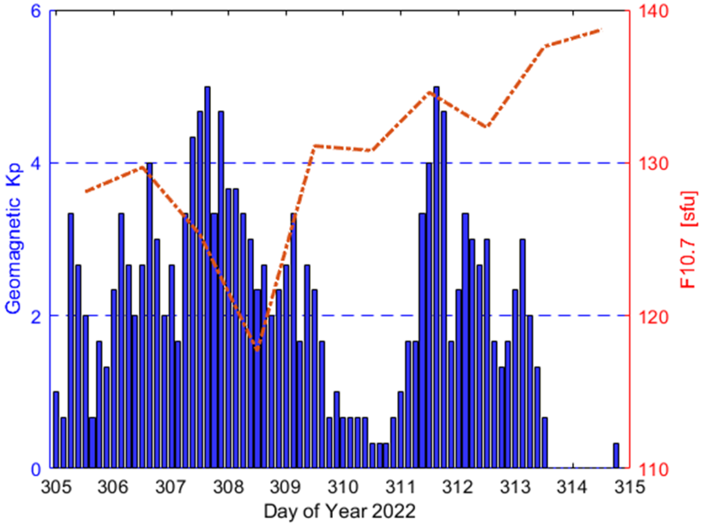
3.1. Experiment Datasets

Twenty-two MGEX stations located in Europe were selected to build a regional reference network. The distribution of these multi-GNSS monitoring stations is shown in Figure 1. It should be noted that 18 blue stations are used for modeling the regional RT between-satellite SD ionospheric delays, and 4 red stations are used to carry out the multi-GNSS RT SF-PPP based on the between-satellite SD ionospheric constraints. The experimental period was set between DoY (Day of Year) 305 to 314 in 2022. The ionospheric conditions over these days can be presented in Figure 2. Except for DoY 310 and 314, the ionosphere is relatively active on all other dates, with over half of the geomagnetic Kp values exceeding 2. Especially on the DoY 307 and 311, some Kp values may even up to 4–5 and indicating intense ionospheric activity. Corresponding, the relatively high solar activity can be observed during the testing period since the most F10.7 index more than 20.

3.2. Processing Strategies

In the processing of multi-GNSS RT SF-PPP, both satellite positions and clocks are fixed by using broadcast ephemeris and CNES (Centre National d’Etudes Spatiales) state space representation (SSR) corrections [2,22]. The satellite DCB can be corrected using the code bias products of CNES SSR in real-time. The weight of observations for different satellites is set using the elevation-dependent weighting model, and the priori precision of code and phase observations are set to 0.3 and 0.003 m, respectively [8]. Considering the lower accuracy of SSR orbits and clocks for BDS-3 inclined geosynchronous orbit (IGSO) satellites (i.e., C38-40), the weight of IGSO observations needs to be set as 1/2 of other medium earth orbit (MEO) satellites [23]. In order to accurately evaluate the positioning accuracy, the precise coordinates of all selected MGEX stations within accuracy of a few mm can be obtained from the SINEX file. Table 1 summarizes some key processing strategies and correction models. In addition, some minor corrections such as relativistic effect and tidal errors are also considered in the positioning domain [24]. The phase wind-up is corrected by using the method of literature [25].

4. Results and Discussion

Before establishing regional RT between-satellite SD ionospheric model, it is necessary to investigate the current positioning accuracy of the multi-GNSS RT SF UU-PPP that can be achieved. Next, both internal and external accord accuracies of the regional RT between-satellite SD ionospheric model need to be evaluated. At last, using the high-precision GRAPHIC (GRoup And PHase Ionospheric Correction) SF-PPP model as a reference, the advantages of the SD ionospheric-constrained RT SF-PPP in terms of convergence and positioning accuracy are analyzed and discussed.

4.1. Performance of the Multi-GNSS Real-Time Single-Frequency UU-PPP in Static Mode

The multi-GNSS observations of 4 red stations shown in Figure 1 for 10 consecutive days (DoY 305-314, 2022) are selected for conducting the GPS + Galileo + BDS-3 static RT SF UU-PPP based on the GPS Klobuchar constraints. Figure 3 gives the time series of RMS positioning errors during the first 3 h, as well as the positioning accuracy in the north (N), east(E), and up(U) directions after 3 h of convergence. It should be noted that the RMS positioning errors for each epoch are calculated from the results of 4 red stations over a period of 10 days. We can see that the vertical (i.e., U direction) RMS positioning error can converge to 10 cm within about 60 min, while for the horizontal component (i.e., the combined error of N and E directions), it takes at least 90 min to reach the same level. After 90 min of convergence, the vertical RMS positioning error can be stabled at approximately 8 cm, but there is still a downward trend in the horizontal component. The horizontal RMS positioning error can be decreased to 6 cm after 180 min of convergence. When conducting RMS statistics on the positioning errors of 3–24 h for each station in consecutive 10 days, the optimal positioning accuracy can be less than 2 cm in horizontal and 4 cm in vertical. The average RMS positioning accuracy of all used stations can reach 2.6, 2.6 and 5.8 cm in the N, E, and U directions, respectively. This indicates that multi-GNSS static RT SF-PPP has the ability to provide reliable cm-level positioning accuracy at present. If the monitoring station positions are fixed to the SINEX precise coordinates rather than estimated as unknown parameters, the higher precision ionospheric observables can be achieved using the multi-GNSS RT SF-PPP technology.

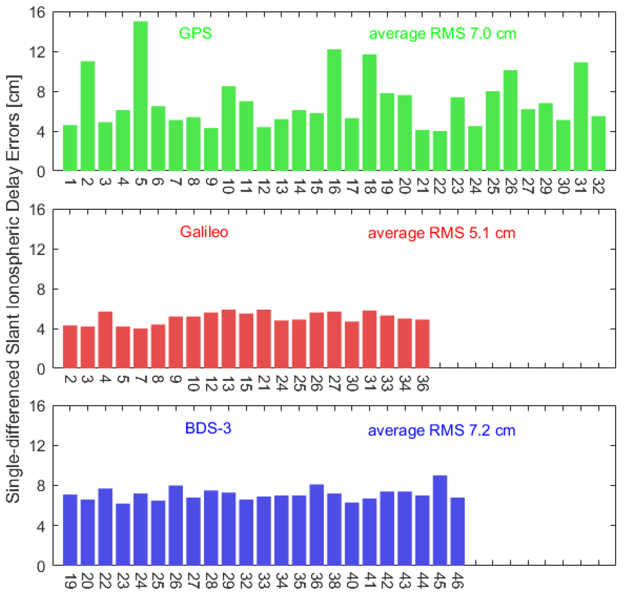
4.2. Internal Accord Accuracy of the Regional Real-Time between-Satellite Single-Differenced Ionospheric Model

To evaluate the performance of the regional RT between-satellite SD ionospheric model proposed in this study, its internal accord accuracy as a key indicator needs to be computed. We first extract the slant ionospheric observables of all visible satellites using SF UU-PPP method. Then, the between-satellite SD slant ionospheric delays of each satellite can be obtained after choosing the reference satellite with highest elevation, which are regarded as reference values. If the between-satellite SD slant ionospheric delays are directly derived from the regional SD ionospheric model established by 22 monitoring stations, these results are called model values. The difference between the above reference values and model values can reflect the internal accord accuracy of the regional RT between-satellite SD ionospheric model. Figure 4 shows the time series of between-satellite SD slant ionospheric errors for GPS, BDS-3, and Galileo satellites in DoY 305, 2022. It should be noted that the different colored points represent the results of different satellites. Considering the slow convergence time of the RT SF-PPP, only the extracted ionospheric observables after 3 h are used to establish the regional RT between-satellite SD ionospheric model. It can be seen that the internal accord accuracy of Galileo satellites is better than that of GPS and BDS-3 satellites for all selected stations, its more than half of errors can be lower than 0.1 m. However, the majority of between-satellite SD slant ionospheric errors for both GPS and BDS-3 satellites only maintained within 0.2 m. The proportion of GPS internal accord accuracy exceeding 0.4 m is larger than that of other constellations. This is reasonable that the number of available GPS satellites is significantly more than other constellations, and more results can be displayed in the time series of Figure 4.
The RMS of between-satellite SD slant ionospheric errors calculated from results of 4 selected stations on 10 days are shown in Figure 5. There is a significant difference in the internal accord accuracy of different GPS satellites. The RMS of between-satellite SD slant ionospheric errors for most GPS satellites is lower than 8 cm, while for G05 satellite, its RMS can be up to 15 cm. In contrast, the difference of internal accord accuracy for Galileo and BDS-3 satellites is not much, its RMS is maintained at around 5 cm for Galileo satellites and can be lower than 8 cm for BDS-3 satellites. The average RMS of between-satellite SD slant ionospheric errors for all GPS, Galileo, and BDS-3 satellites are 7.0, 5.1, 7.2 cm, respectively. This proves that the internal accord accuracy of the regional RT between-satellite SD ionospheric model using multi-GNSS SF observations can be better than 0.5 TECU (1 TECU ≈ 15.6 cm).

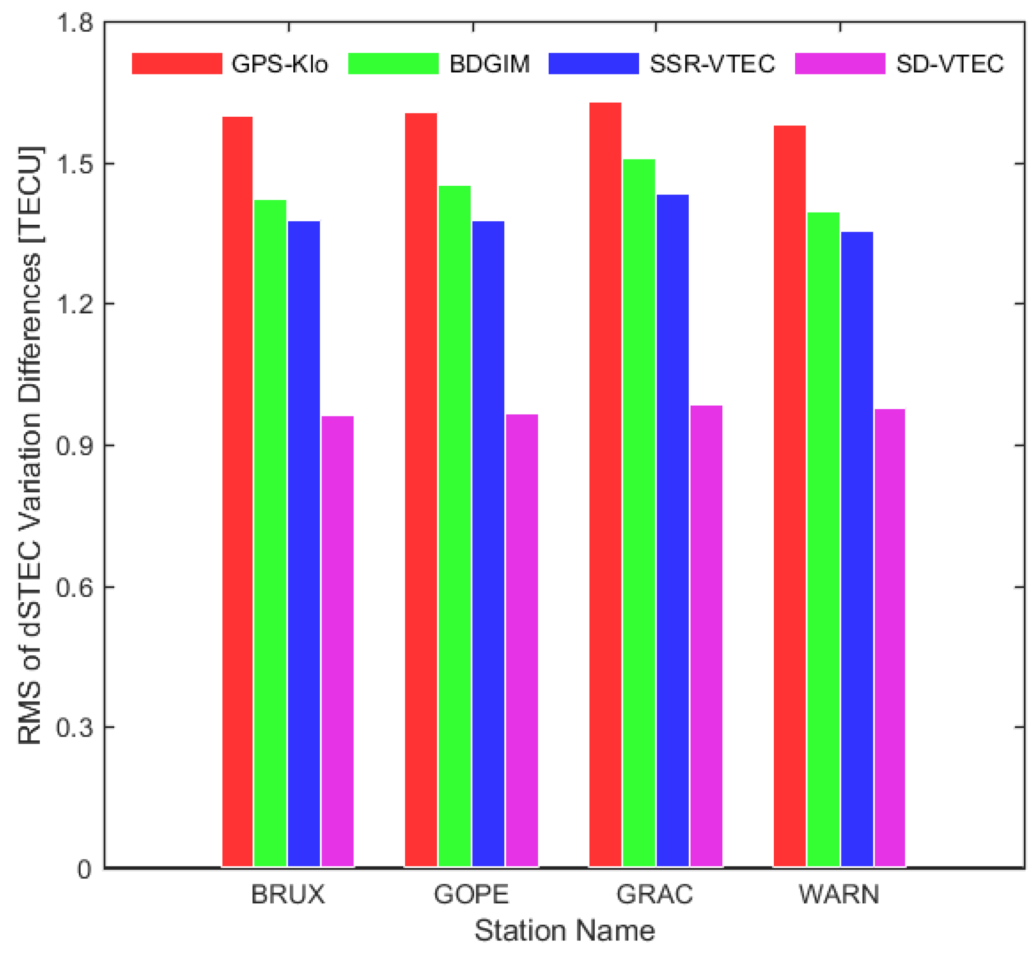
4.3. External Accord Accuracy of the Regional Real-Time between-Satellite Single-Differenced Ionospheric Model

Although the internal accord accuracy of the regional RT between-satellite SD ionospheric model has excellent performance, its true accuracy still needs to be validated by external accord accuracy. Considering that the differential STEC (dSTEC) derived from epoch-differenced geometry-free (GF) combinations of phase observations have mm-level accuracy, the variation of dSTEC can be further obtained from the between-satellite SD algorithm [29]. This between-satellite SD dSTEC can ebe regarded as reference value. For the regional RT between-satellite SD ionospheric model, the between-satellite SD slant ionospheric delay can be directly calculated, and then the model value of dSTEC variation was obtained using the epoch-differenced method [19]. Similarly, the above model value of dSTEC variation can be calculated from the GPS Klobuchar, BDGIM, and CNES SSR VTEC ionospheric models. Therefore, the difference between the model and reference values can be defined as an indicator of external accord accuracy. Figure 6 shows the differences in dSTEC variation of 4 red stations using GPS, Galileo, and BDS-3 satellites. It is worthing that the calculate interval of external accord accuracy was set to 5 min and the results of elevation exceeding 10 degrees are removed in this assessment. The abbreviation for “GPS-Klo” and “SD-VTEC” are represented as the GPS Klobuchar model and the regional RT between-satellite SD ionospheric model, respectively. We can see that the dSTEC variation differences of different stations have similar distribution, and their values decrease with the increase of elevation. The dSTEC variation differences of the GPS Klobuchar model have the maximum range and even exceed ±5 TECU. There is not much difference in external accord accuracy among the GPS Klobuchar, BDGIM and SSR VTEC models. Compared with the above three models, the variation range of the regional RT between-satellite SD ionospheric model in external accord accuracy is mainly concentrated in ±2 TECU and can be lower than 1 TECU at high elevation. This indicates that the regional RT between-satellite SD ionospheric model has higher accuracy as expected.
The RMS of dSTEC variation differences for all selected ionospheric models using 4 red stations throughout the entire testing period is given in Figure 7. Except for the regional RT between-satellite SD ionospheric model with RMS value of below 1.0 TECU, the RMS of dSTEC variation differences for all other ionospheric models is more than 1.3 TECU and even up to 1.6 TECU. The average RMS values of all stations in external accord accuracy are 1.60, 1.44, 1.39, and 0.96 TECU for the GPS Klobuchar, BDGIM, SSR VTEC, and regional RT between-satellite SD ionospheric models, respectively. This result demonstrates the feasiblilty of modeling the high-precision ionospheric delay using multi-GNSS SF observations.

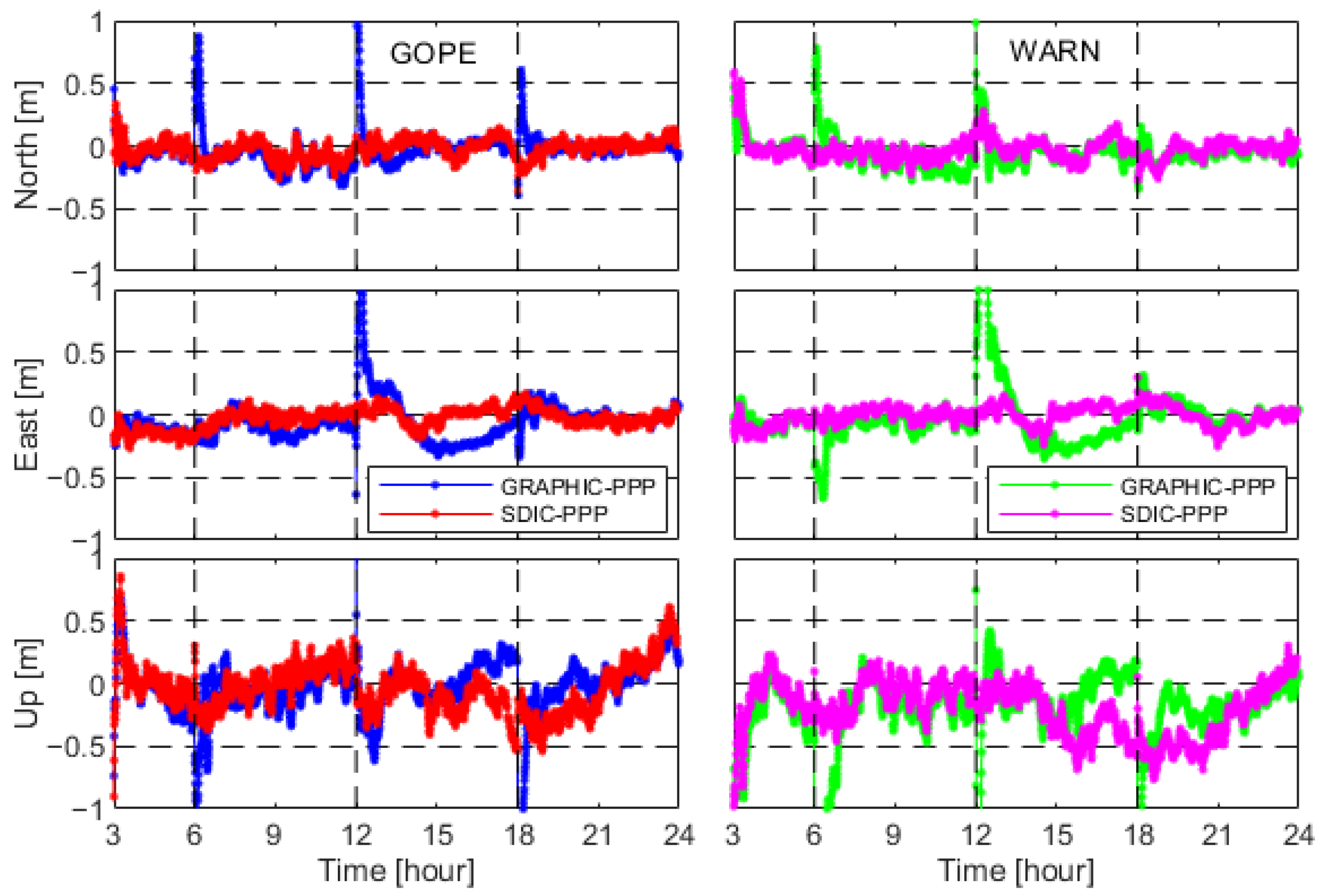
4.4. Multi-GNSS Real-Time Single-Frequency PPP Based on the Regional between-Satellite Single-Differenced Ionospheric Constraints

As long as the accuracy of external ionospheric constraints is high enough, the positioning accuracy and (re-)convergence of the UU-PPP can be improved in theory [30]. In order to explore the advantages of the SD ionospheric constrained multi-GNSS RT SF-PPP, the results of high-precision GRAPHIC RT SF-PPP can be used as a reference. Due to the significant influence of code observation noise on the GRAPHIC model, an RT phase smoothing code observation method named CNMC (Code Noise and Multipath Correction) filter was adopted to further improve the performance of the GRAPHIC RT SF-PPP in this study [31]. Figure 8 shows the daily solutions of the GPS + Galileo + BDS-3 RT SF-PPP in kinematic mode for 2 red stations on DoY 305, 2022. It should be noted that all available satellites are reinitialized with the interval of 6 h to simulate GNSS signal interruption or missing. It is very clear to see that the positioning errors of the GRAPHIC SF-PPP at reinitialized epoch is significantly larger than that of the SD ionospheric-constrained (SDIC) SF-PPP and even exceed 1 m. No matter what SF-PPP models, the positioning accuracy of horizontal component is better than that of vertical component. After convergence, the horizontal and vertical positioning errors can be stable within around 0.2 and 0.5 m, respectively. This indicates that both GRAPHIC and SDIC RT SF-PPP models have the ability to achieve dm-level positioning accuracy in kinematic mode at present.
The convergecne curve of the GPS + Galileo + BDS-3 RT SF-PPP in kinematic mode at 68% confidence level is displayed in Figure 9. The absolute positioning errors of 4 red stations during the whole testing period are sorted from small to large at each epoch, and the 68th% of absolute positioning errors for each epoch is selected as representative to measure the convergence performance [20]. We can see that the horizontal positioning errors of the GRAPHIC and SDIC RT SF-PPP remain consistent in the initialization period, but the vertical positioning errors of the SDIC RT SF-PPP are always smaller than those of the GRAPHIC model during the first 50 min. In the case of setting 0.2 m as the convergence criterion of positioning errors, the convergence time of the SDIC RT SF-PPP with 37 min is less than that of the GRAPHIC RT SF-PPP with 47 min, and its improvement of convergecne speed can up to 21.3%. In the period of re-convergence, due to the introduction of the regional RT bettween-satellite SD ionospheric model, both horizontal and vertcial positioning errors of the SDIC RT SF-PPP can be maintained within 0.2 m. Such excellent positioning performance is significantly superior to the GRAPHIC model, which takes at least 75 min to converge to 0.2 m. This indicates that the positioning errors of the SDIC RT SF-PPP model hardly generate fluctuations when some GNSS signals missing or blocked in the complex kinematic environments.
Figure 10 shows the RMS of positioning errors of GPS + Galileo + BDS-3 kinematic RT SF-PPP after convergence of 3 h, and these values are calculated from results of 4 red stations on 10 days. It can be seen that both N and E positioning accuracies of the SDIC RT SF-PPP is better than that of the GRAPHIC model, and its corresponding improvements are 17.0% and 45.7% respectively. However, compared with the GRAPHIC model, the vertical positioning accuracy of the SDIC RT SF-PPP is decreased from 0.21 to 0.26 m, which is caused by the limited accuracy of the regional RT between-satellite SD ionospheric model. If the multi-GNSS DF observations rather than SF observations are used to establish this regional SD ionospheri model, the vertical positioning accuracy of the SDIC RT SF-PPP can be improved like results of [19]. Therefore, this novel multi-GNSS RT SF-PPP model proposed in this study is mainly benefit to improving the horizontal positioning accurcy, with an improvement rate of 37.9%. From the perspective of 3D comprehensive error, the SDIC RT SF-PPP has slighly better accuracy and can reach within 0.3 m.

5. Conclusions

Due to the limited accuracy of ionospheric observables extracted by the CCL method, the UU-PPP technology has gradually become an important solution for extracting high-precision slant ionospheric delays in recent years. Different from the previse research using GNSS DF or multi-frequency (MF) observations, the multi-GNSS SF UU-PPP was used to extract the ionospheric observables in this study. To completely remove the negative effects of receiver DCB with short-term time-varying characteristics, the between-satellite SD method can be adopted for establishing the regional RT ionospheric model. In this contribution, we evaluate the performance of the regional RT between-satellite SD ionospheric model and explore its contribution to the multi-GNSS RT SF-PPP.
The internal accord accuracy of the SD slant ionospheric delays derived from the regional RT between-satellite SD ionospheric model can be better than 0.5 TECU, and its average RMS of GPS, BDS-3, and Galileo satellites are 7.0, 7.2, and 5.1 cm, respectively. Using the dSTEC variation calculated from between-satellite SD and epoch-differenced GF phase observations as a refence, the external accord accuracy of this ionospheric model proposed in this study is significantly better than that of the GPS Klobuchar, BDGIM, and CNES SSR VTEC models, and its average RMS of less than 1.0 TECU can be achieved.
With the introduction of the regional RT between-satellite SD ionospheric model into the multi-GNSS RT SF-PPP in kinematic mode, its initialization speed of vertical positioning errors can be improved by 21.3% to 37 min in comparison with the CNMC-smoothed GRAPHIC model. More importantly, both horizontal and vertical positioning errors of the SDIC SF-PPP after reinitialization can be maintained within 0.2 m. This means that proposed SDIC SF-PPP model has the ability to enhance the continuity and stability of kinematic positioning in case of some satellites missing or blocked. After convergence, the horizontal positioning accuracy of the SDIC SF-PPP can be improved by 37.9% to 0.13 m compared to the GRAPHIC model, but its vertical positioning accuracy may be decreased. With the increase of the number of monitoring stations in the region or the improvement of RTS products quality, the spatial-temporal resolution and accuracy of extracted ionospheric observables can be improved, and result in higher accuracy of the SD ionospheric model. As long as the SD ionospheric model is accurate enough, the vertical positioning accuracy of the SD ionospheric-constrained RT SF-PPP can be improved. In summary, the 3D positioning accuracy of the SDIC SF-PPP can be better than 0.3 m and is superior to other widely used SF-PPP models. To verify the effectiveness of the proposed algorithm on real low-cost SF-PPP users, the truly SF observations collected from the affordable SF devices or chips need to be used for carrying out RT SF-PPP tests in our future research.

Author Contributions

Conceptualization, A.W.; methodology, A.W. and X.L.; software, A.W. and Y.Z.; data curation, A.W. and X.L.; validation, X.L. and H.W.; formal analysis, A.W., Y.Z. and X.L.; writing—original draft preparation, A.W.; writing—review and editing, Y.Z., X.L. and H.W.; supervision, J.C.; funding acquisition, A.W., J.C., X.L. and H.W. All authors have read and agreed to the published version of the manuscript.

Funding

This research was funded by the National Natural Science Foundation of China (No. 42304023), National Natural Science Foundation of China (No. 42304015), National Natural Science Foundation of China (No. 42274044), China Postdoctoral Science Foundation (No. 2022M723404), Program of Shanghai Academic/Technology Research Leader (No. 20XD1404500); Jiangsu Province Natural Science Foundation of China (No. BK20231087); Open Research Foundation of the State Key Laboratory of Geodesy and Earth’s Dynamics (No. SKLGED2024-3-7).

Data Availability Statement

The datasets analyzed in this study are managed by IGS, and data will be made available on request.

Acknowledgments

The authors would like to thank the IGS, CNES, and MGEX for the provision of GNSS observation data, broadcast ephemeris, real-time SSR corrections, GPS Klobuchar and BDGIM model coefficients.

Conflicts of Interest

The authors declare no conflicts of interest.

References

  1. Hernandez-Pajares, M.; Juan, J.M.; Sanz, J.; Aragon-Angel, A.; Garcia-Rigo, A.; Salazar, D.; Escudero, M. The ionosphere: Effects, GPS modeling and the benefits for space geodetic techniques. J. Geod. 2011, 85, 887–907. [Google Scholar] [CrossRef]
  2. Wang, A.; Chen, J.; Zhang, Y.; Meng, L.; Wang, B.; Wang, J. Evaluating the impact of CNES real-time ionospheric products on multi-GNSS single-frequency positioning using the IGS real-time service. Adv. Space Res. 2020, 66, 2516–2527. [Google Scholar] [CrossRef]
  3. Odolinski, R.; Teunissen, P.J.G. An assessment of smartphone and low-cost multi-GNSS single-frequency RTK positioning for low, medium and high ionospheric disturbance periods. J. Geod. 2018, 93, 701–722. [Google Scholar] [CrossRef]
  4. Zou, J.; Wang, A.; Wang, J. Single-Frequency Precise Point Positioning Using Regional Dual-Frequency Observations. Sensors 2021, 21, 2856. [Google Scholar] [CrossRef]
  5. Klobuchar, J.A. Ionospheric time-delay algorithm for single frequency GPS users. IEEE Trans. Aerosp. Electron. Syst. 1987, 23, 325–331. [Google Scholar] [CrossRef]
  6. Yuan, Y.; Wang, N.; Li, Z.; Huo, X. The BeiDou global broadcast ionospheric delay correction model (BDGIM) and its preliminary performance evaluation results. Navigation 2019, 66, 55–69. [Google Scholar] [CrossRef]
  7. Bidaine, B.; Warnant, R. Ionosphere modelling for Galileo single frequency users: Illustration of the combination of the NeQuick model and GNSS data ingestion. Adv. Space Res. 2011, 47, 312–322. [Google Scholar] [CrossRef]
  8. Wang, A.; Zhang, Y.; Chen, J.; Li, S.; Zhang, Z.; Wang, H. Analysis of spatial–temporal characteristics for BDS-3 broadcast ionospheric models (BDS Klobuchar and BDGIM) in multi-GNSS real-time single-frequency precise point positioning. Measurement 2024, 224, 113958. [Google Scholar] [CrossRef]
  9. Cai, C.; Gong, Y.; Gao, Y.; Kuang, C. An approach to speed up single-frequency PPP convergence with quad-constellation GNSS and GIM. Sensors 2017, 17, 1302. [Google Scholar] [CrossRef]
  10. Liu, Q.; Hernández-Pajares, M.; Yang, H.; Monte-Moreno, E.; Roma-Dollase, D.; García-Rigo, A.; Li, Z.; Wang, N.; Laurichesse, D.; Blot, A.; et al. The cooperative IGS RT-GIMs: A reliable estimation of the global ionospheric electron content distribution in real time. Earth Syst. Sci. Data 2021, 13, 4567–4582. [Google Scholar] [CrossRef]
  11. Chen, L.; Yi, W.; Song, W.; Shi, C.; Lou, Y.; Cao, C. Evaluation of three ionospheric delay computation methods for ground-based GNSS receivers. GPS Solut. 2018, 22, 125. [Google Scholar] [CrossRef]
  12. Li, Z.; Wang, N.; Hernandez-Pajares, M.; Yuan, Y.; Krankowski, A.; Liu, A.; Zha, J.; Garcia-Rigo, A.; Roma-Dollase, D.; Yang, H.; et al. IGS real-time service for global ionospheric total electron content modeling. J. Geod. 2020, 94, 32. [Google Scholar] [CrossRef]
  13. Zhang, B.; Ou, J.; Yuan, Y.; Li, Z. Extraction of line-of-sight ionospheric observables from GPS data using precise point positioning. Sci. China Earth Sci. 2012, 55, 1919–1928. [Google Scholar] [CrossRef]
  14. Liu, T.; Zhang, B.; Yuan, Y.; Li, M. Real-time precise point positioning (RTPPP) with raw observations and its application in real-time regional ionospheric VTEC modeling. J. Geod. 2018, 92, 1267–1283. [Google Scholar] [CrossRef]
  15. Wang, N.; Yuan, Y.; Li, Z.; Montenbruck, O.; Tan, B. Determination of differential code biases with multi-GNSS observations. J. Geod. 2016, 90, 209–228. [Google Scholar] [CrossRef]
  16. Li, M.; Yuan, Y.; Zhang, X.; Zha, J. A multi-frequency and multi-GNSS method for the retrieval of the ionospheric TEC and intraday variability of receiver DCBs. J. Geod. 2020, 94, 102. [Google Scholar] [CrossRef]
  17. Zhang, B.; Zhao, C.; Odolinski, R.; Liu, T. Functional model modification of precise point positioning considering the time-varying code biases of a receiver. Satell. Navig. 2021, 2, 11. [Google Scholar] [CrossRef]
  18. Xiang, Y.; Gao, Y.; Li, Y. Reducing convergence time of precise point positioning with ionospheric constraints and receiver differential code bias modeling. J. Geod. 2020, 94, 8. [Google Scholar] [CrossRef]
  19. Wang, A.; Zhang, Y.; Chen, J.; Wang, H. Improving the (re-)convergence of multi-GNSS real-time precise point positioning through regional between-satellite single-differenced ionospheric augmentation. GPS Solut. 2022, 26, 39. [Google Scholar] [CrossRef]
  20. Wang, A.; Zhang, Y.; Chen, J.; Wang, H.; Yuan, D.; Jiang, J.; Zhang, Z. Investigating the contribution of BDS-3 observations to multi-GNSS single-frequency precise point positioning with different ionospheric models. Adv. Space Res. 2024, 73, 553–570. [Google Scholar] [CrossRef]
  21. Chen, J.; Zhang, Y.; Yu, C.; Wang, A.; Song, Z.; Zhou, J. Models and performance of SBAS and PPP of BDS. Satell. Navig. 2022, 3, 4. [Google Scholar] [CrossRef]
  22. Kazmierski, K.; Sosnica, K.; Hadas, T. Quality assessment of multi-GNSS orbits and clocks for real-time precise point positioning. GPS Solut. 2018, 22, 11. [Google Scholar] [CrossRef]
  23. Chen, J.; Wang, J.; Yu, C.; Zhang, Y.; Wang, B. Improving BDS broadcast ephemeris accuracy using ground-satellite-link observations. Satell. Navig. 2022, 3, 11. [Google Scholar] [CrossRef]
  24. Petit, G.; Luzum, B. IERS Conventions; IERS Technical 2010 Note 36; Verlag des Bundesamts für Kartographie und Geodäsie: Frankfurt am Main, Germany, 2010. [Google Scholar]
  25. Wu, J.T.; Wu, S.C.; Hajj, G.A.; Bertiger, W.I.; Lichten, S.M. Effects of antenna orientation on GPS carrier phase. In Proceedings of the AAS/AIAA Astrodynamics Conference, Durango, CO, USA, 1992; pp. 1647–1660. [Google Scholar]
  26. Boehm, J.; Moller, G.; Schindelegger, M.; Pain, G.; Weber, R. Development of an improved empirical model for slant delays in the troposphere (GPT2w). GPS Solut. 2015, 19, 433–441. [Google Scholar] [CrossRef]
  27. Zhou, F.; Dong, D.; Li, P.; Li, X.; Schuh, H. Influence of stochastic modeling for inter-system biases on multi-GNSS undifferenced and uncombined precise point positioning. GPS Solut. 2019, 23, 59. [Google Scholar] [CrossRef]
  28. Lu, Y.; Yang, H.; Li, B.; Li, J.; Xu, A.; Zhang, M. Analysis of Characteristics for Inter-System Bias on Multi-GNSS Undifferenced and Uncombined Precise Point Positioning. Remote Sens. 2023, 15, 2252. [Google Scholar] [CrossRef]
  29. Feltens, J.; Angling, M.; Jackson-Booth, N.; Jakowski, N.; Hoque, M.; Hernandez-Pajares, M.; Aragon-Angel, A.; Orus, R.; Zandbergen, R. Comparative testing of four ionospheric models driven with GPS measurements. Radio. Sci. 2011, 46, 1–11. [Google Scholar] [CrossRef]
  30. Li, B.; Zang, N.; Ge, H.; Shen, Y. Single-frequency PPP models: Analytical and numerical comparison. J. Geod. 2019, 93, 2499–2514. [Google Scholar] [CrossRef]
  31. Chang, Z.; Hu, X.; Guo, R.; Cao, Y.; Wu, X.; Wang, A.; Dong, E. Comparison between CNMC and hatch filter & its precision analysis for BDS precise relative positioning. Sci. Sin. Phys. Mech. Astron. 2015, 45, 079508. (In Chinese) [Google Scholar]
Figure 1. Distribution of the selected 22 MGEX stations in Europe.
Remotesensing 16 01511 g001
Figure 2. Geomagnetic Kp values and F10.7 index during the testing period.
Remotesensing 16 01511 g002
Figure 3. RMS of positioning errors during the first 3 h and positioning accuracy of each station after 3 h convergence in multi-GNSS static RT SF UU-PPP (DoY 305-314, 2022).
Remotesensing 16 01511 g003
Figure 4. Time series of between-satellite SD slant ionospheric errors for different GNSS satellites at (a) BRUX, (b) GOPE, (c) GRAC, and (d) WARN stations in DoY 305, 2022.
Remotesensing 16 01511 g004aRemotesensing 16 01511 g004b
Figure 5. RMS of between-satellite SD slant ionospheric errors for different GNSS satellites (4 red stations in DoY 305-314, 2022).
Remotesensing 16 01511 g005
Figure 6. Differences in dSTEC variation of GPS, Galielo, and BDS-3 satellites at 4 red stations (DoY 305, 2022).
Remotesensing 16 01511 g006
Figure 7. RMS of dSTEC variation differences using different ionospheric models at 4 red stations (DoY 305-314, 2022).
Remotesensing 16 01511 g007
Figure 8. Kinematic positioning errors of both GRAPHIC and SDIC RT SF-PPP using GPS + Galileo + BDS-3 observations at GOPE and WARN stations (DoY 305, 2022).
Remotesensing 16 01511 g008
Figure 9. Convergence curve of GPS + Galileo + BDS-3 RT SF-PPP in kinematic mode at 68% confidence level during the first 3 h (4 red stations in DoY 305-314, 2022).
Remotesensing 16 01511 g009
Figure 10. RMS positioning accuracy of GPS + Galileo + BDS-3 RT SF-PPP in kinematic mode after convergence of 3 h (4 red stations in DoY 305-314, 2022).
Remotesensing 16 01511 g010
Table 1. Processing strategies and correction models of the multi-GNSS RT SF-PPP.
ItemsStrategies or Models
ObservationGPS: L1; Galileo: E1; BDS-3: B1I
Sampling rate30 s
Elevation cutoff angle10°
Antenna correctionCorrected by igs14_2233.atx
Dry part of tropospheric delayCorrected by GPT2w + SAAS + VMF models [26]
Wet part of tropospheric delayEstimated as random-walk noise
Ionospheric delayCorrected by GPS Klobuchar model
Residual of ionospheric delayEstimated as random-walk noise [19]
Positioning estimatorKalman filter
Receiver coordinatesEstimated as white noise
Receiver clocksEstimated as white noise
ISBEstimated as random-walk noise [27,28]
Phase ambiguitiesEstimated as float constant
Disclaimer/Publisher’s Note: The statements, opinions and data contained in all publications are solely those of the individual author(s) and contributor(s) and not of MDPI and/or the editor(s). MDPI and/or the editor(s) disclaim responsibility for any injury to people or property resulting from any ideas, methods, instructions or products referred to in the content.

