


Investigation on the Utilization of Millimeter-Wave Radars for Ocean Wave Monitoring


1
Faculty of Information Science and Engineering, Ocean University of China, Qingdao 266100, China
2
The Laboratory for Regional Oceanography and Numerical Modeling, Laoshan Laboratory, Qingdao 266237, China
3
College of Engineering, Ocean University of China, Qingdao 266100, China
*
Author to whom correspondence should be addressed.
Remote Sens. 2023, 15(23), 5606; https://0-doi-org.brum.beds.ac.uk/10.3390/rs15235606
Submission received: 30 October 2023
/
Revised: 24 November 2023
/
Accepted: 30 November 2023
/
Published: 2 December 2023
(This article belongs to the Special Issue Applications and New Trends in Metrology for Radar/LiDAR-Based Systems II)
Abstract
:The feasibility of using millimeter-wave radars for wave observations was investigated in this study. The radars used in this study operate at a center frequency of 77.572 GHz. To investigate the feasibility of wave observations and extract one-dimensional and two-dimensional wave spectra, arrays consisting of multiple radar units were deployed for observations in both laboratory and field environments. Based on the data measured with the millimeter-wave radars, one-dimensional wave spectra and two-dimensional wave directional spectra were evaluated using the periodogram method and the Bayesian directional spectrum estimation method (BDM), respectively. Meanwhile, wave parameters such as the significant wave height, wave period, and wave direction were also calculated. Via comparative experiments with a capacitive wave height meter in a wave tank and RADAC’s WG5-HT-CP radar in an offshore field, the viability of using millimeter-wave radars to observe water waves was validated. The results indicate that the one-dimensional wave spectra measured with the millimeter-wave radars were consistent with those measured with the mature commercial capacitive wave height meter and the WG5-HT-CP wave radar. Via wave direction measurement experiments conducted in a wave tank and offshore environment, it is evident that the wave directions retrieved with the millimeter-wave radars were in good alignment with the actual wave directions.
1. Introduction
Real-time and all-weather wave height monitoring is fundamental for all coastal and marine activities [1,2]. Currently, contact and non-contact measurements are the two main methods for measuring wave height. Contact measurement methods include pressure sensors, acoustic wave measurement devices, and buoys. Non-contact measurement methods include photogrammetric surveys, laser radars, and satellites equipped with radar altimeters. The pressure-based wave measurement technique is still semi-theoretical and semi-empirical, and calibration methods rely on laboratory simulations [3]. The accuracy of acoustic wave measurement techniques can be affected under adverse weather conditions (such as storms) and in rough sea states (breaking waves) due to unclear water–air interfaces. Wave buoys have matured technologically, but their measurements may be influenced by their movement in short-wave crests [4], and resonance effects can occur under specific wave conditions, thereby affecting the measurement results [5]. Photographic measurements can provide information from a significant portion of the sea surface with high accuracy, but their computational process is cumbersome and constrained by factors such as lighting conditions and camera resolution [6]. Laser measurements can accurately determine the vertical height from the instrument to the sea surface; however, they are sensitive to water quality, and their usage is subject to adverse weather conditions such as wind, rain, and ice [7]. Therefore, it is of paramount importance to explore a novel non-contact device for observing ocean waves, ensuring its immunity to adverse weather conditions and lighting effects while enabling uninterrupted and stable operation throughout the day and night. Additionally, it is crucial to establish a universally applicable data acquisition and processing methodology tailored to this device, thereby obtaining precise wave and directional spectra, which hold significant practical value.
A millimeter-wave radar is a special radar that utilizes short-wavelength electromagnetic waves with a signal wavelength in the millimeter range [8]. However, the propagation of millimeter waves in the atmosphere is subject to large absorption and scattering, which limits their efficiency in long-distance propagation [9], but a millimeter-wave radar has a small antenna size, narrow beamwidth, and high accuracy, providing an all-weather communication capability [10]. In millimeter-wave frequencies, the antenna size and weight can be significantly reduced while providing the same antenna beamwidth and gain [11]. Therefore, a millimeter-wave radar has unique advantages in fields such as hydrology and meteorology. Linear frequency modulation continuous-wave (LFMCW) radar systems measure the distance to a target by analyzing the difference between the transmitted and received signals [12]. LFMCW radars offer advantages such as low transmitter power, high receiver sensitivity, high distance resolution, a simple structure, and ease of integration [13,14,15], making them widely employed in high-precision measurement fields [16,17,18,19,20,21,22,23,24,25].
This study employed a millimeter-wave radar operating at a center frequency of 77.572 GHz to observe the spatiotemporal variations in ocean wave surfaces. Simultaneously, the Bayesian directional spectrum estimation method (BDM) was employed to probe the two-dimensional wave spectra. To validate the reliability of the millimeter-wave radar detection results, we conducted on-site observation experiments both in the wave tank at the Ocean University of China and in nearshore areas. We conducted a comparison between the wave feature parameters and spectral results obtained from millimeter-wave radar observations and those measured with capacitance wave meters and RADAC wave radars. The results show excellent agreement, thereby confirming the practical applicability of millimeter-wave radars in wave observations. The remaining content of this paper is organized as follows: in Section 2, the wave height measurement method based on millimeter-wave radars is introduced; in Section 3, the spectral analysis method and the ocean wave parameters are presented; in Section 4, an analysis and comparison of the millimeter-wave radar experimental results are conducted; and in Section 5, the feasibility of wave observations with millimeter-wave radars is summarized and discussed.
2. Wave Height Measurements Using Millimeter-Wave LFMCW Radars
2.1. Ranging Principle of Millimeter-Wave Radars
A millimeter-wave LFMCW radar measures distances by transmitting a linear-frequency-modulated wave, and the single-chirp linear-frequency-modulated continuous-wave signal is depicted in Figure 1.
Taking the example of a single-sawtooth linear-frequency-modulated continuous wave, the transmission signal is as follows:
in which the effective interval , where represents the chirp period, represents the amplitude of the transmitted signal, represents the starting frequency of the signal, represents the initial phase of the signal, and represents the frequency modulation slope of the signal. Assuming that there is a stationary target in the area illuminated by the radar signal at a distance of from the radar, and the electromagnetic wave propagation speed is , the radar receives the echo signal after passing through a time interval of . Neglecting the initial phase of the transmitted signal, noise during the propagation process, and phase shift caused by target reflection, the echo signal is represented as
where represents the target reflection coefficient. Mixing the transmitted and received signals and performing down-conversion results in the intermediate-frequency (IF) signal of the target:
Due to the electromagnetic wave propagation speed m/s, the small term in Equation (3) has been neglected. Where is the wavelength of the electromagnetic wave, the frequency and initial phase of the intermediate-frequency (IF) signal are related to the distance between the measured object and the radar. The distance can be calculated from the relationship between the frequency or phase of the IF signal. The distance resolution is
where is the bandwidth of the radar signal. The maximum range distance is
where is the analog-to-digital converter (ADC) sampling rate. In Equation (4), the radar’s range resolution is related to the radar bandwidth and, consequently, the chirp rate and pulse duration. Increasing the radar bandwidth can result in a smaller range resolution, but it may violate the Nyquist sampling theorem, decreasing the maximum detection range. According to the radar equation [26], the maximum detectable range of the radar is related to parameters such as the radar detection threshold (), radar cross-section (), peak transmit power (), antenna gain (), and radar losses (). However, from a signal perspective, increasing the sampling frequency and reducing the chirp rate can enhance the radar’s maximum detection range. When the pulse duration remains constant, a conflict arises between the radar’s maximum detectable range and range resolution. Additionally, increasing the observation time while keeping the sampling frequency constant results in a greater number of ADC samples, which presents challenges in terms of data transmission and computer processing, ultimately limiting the radar’s real-time capability. Therefore, a trade-off needs to be made for parameters and . The radar parameters employed in this study are listed in Table 1.
To enhance the signal-to-noise ratio, every frame comprised 10 chirps for coherent accumulation, and the frame period was set at 50 ms.
2.2. Wave Height Information Extraction
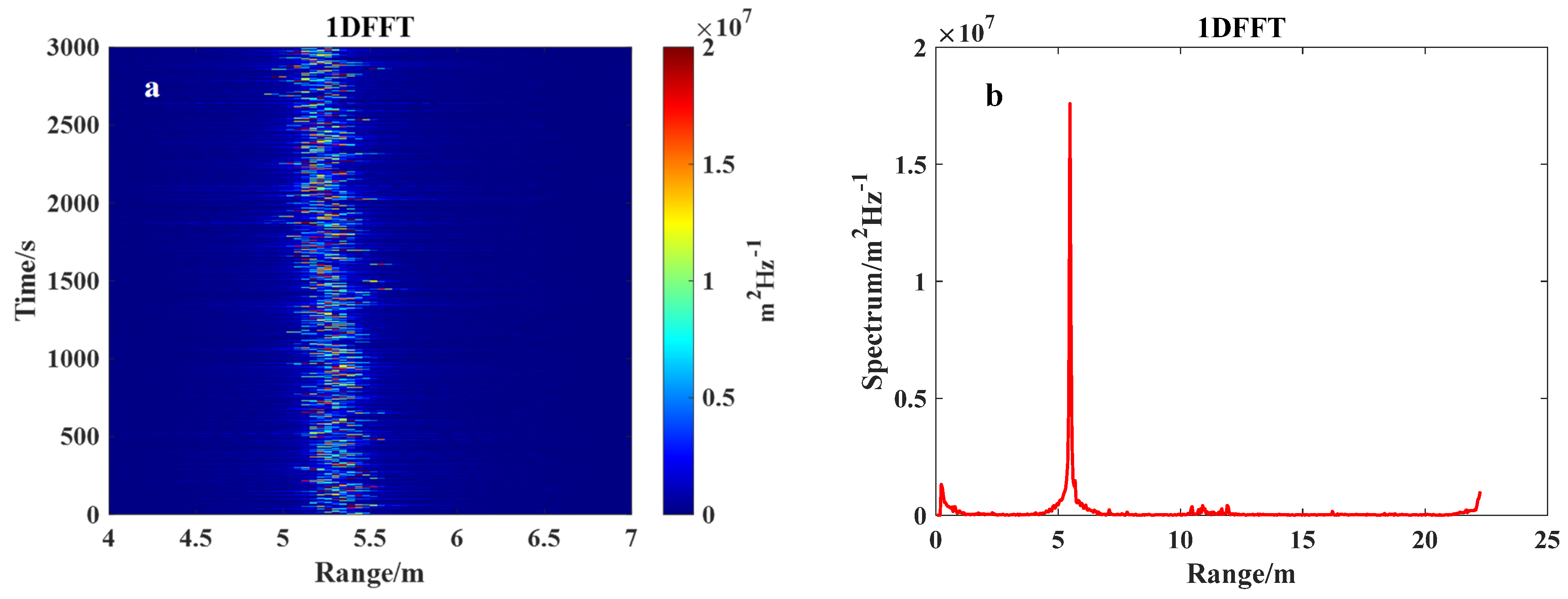
The radars emitted linear-frequency-modulated signals, and an array of three millimeter-wave radars received echo information from different locations. The received signals underwent chirp compression and heterodyne mixing, followed by the pulse accumulation of the heterodyned intermediate-frequency (IF) signals. One-dimensional range profiles were obtained via Fourier transformation, and a peak search was performed to determine the instantaneous distance between the radar and the sea surface. Within the radar beamwidth, the echo signal from a moving sea surface can span several range bins and exhibits random variations in range [27]. There are echoes from scattering points within the entire beam width. Under the experimental conditions of this article, the echo of the signal within the footprint was closer to the average sea level inside the footprint, not the highest sea level. The millimeter-wave radar was positioned above the sea surface with a sampling frequency of 5000 KHz and a chirp slope of 33.71 MHz/. Figure 2a presents the waveforms of multiple chirps measured with the millimeter-wave radar on the sea surface, while Figure 2b displays the waveform of one of these chirps.
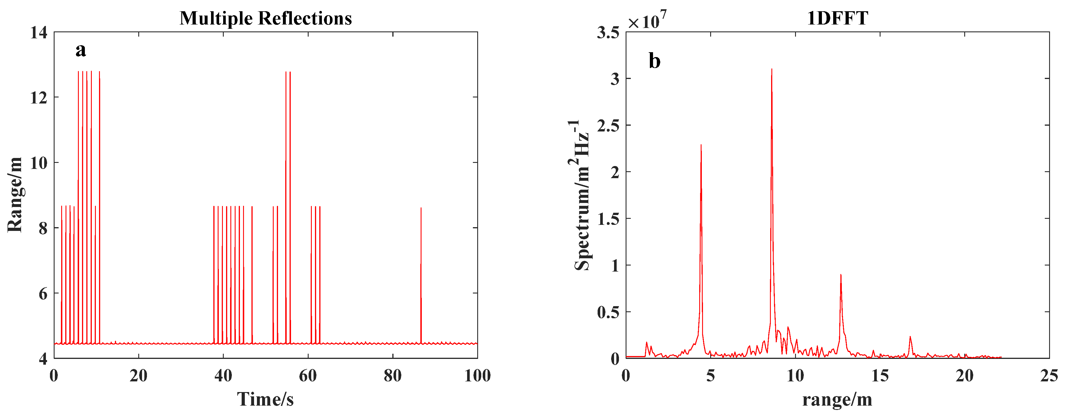
In the process of using the millimeter-wave radar to measure ocean waves, we observed that signals can be reflected between the water surface and the platform’s bottom. Furthermore, there exist secondary or multiple reflections, sometimes stronger than the first reflection, which could lead to significant errors in the inverted wave spectra and wave parameters. Figure 3a depicts the occurrence of multiple reflections when the radar is placed on a metal platform for wave measurements. In this case, with the radar placed approximately 20 cm away from the metal platform, the phenomenon illustrated in Figure 3b emerges: the strength of the second-order reflection in the radar echo is greater than that of the first-order reflection. Therefore, when situating a millimeter-wave radar, it should be placed as far as possible from metallic platforms, and signal correction should be applied in the subsequent processing.
3. Ocean Wave Spectrum and Wave Direction Spectrum Analysis
The utilization of spectra to describe waves and compute wave parameters holds significant theoretical and practical significance in studying ocean waves. The wave spectrum can be obtained via the correlation function using fixed-point wave records [28,29], and the periodogram method is currently the primary approach to obtaining a wave spectrum. Partial computational results from the study by Fan [30] indicated that the spectral peaks and shapes of wave spectra obtained using the covariance function method and the periodogram method are relatively close. The wave direction spectrum provides information about the distribution of wave energy in both frequency and direction. Estimating the wave direction spectrum from limited data [31] can be achieved using various methods, including the maximum likelihood method (MLM) [32,33], the extended maximum entropy principle method (EMEP) [34], and the Bayesian directional spectrum estimation method (BDM) [35], among others. The BDM shows good reproducibility and stability when calculating an ocean wave direction spectrum [36]. To minimize the differences caused by using different processing methods, the preprocessed data in this study were analyzed using the periodogram method to calculate the wave spectrum, and the BDM was employed to calculate the wave direction spectrum.
3.1. The Wave Spectrum Based on the Periodogram Method
The wave spectrum was calculated using the periodogram method [37] based on the following principles:
where represents the displacement of the wave surface measured. represents the duration of observation.
The spectral estimation formula is given as follows:
where represents the displacement of the wave surface measured with the millimeter-wave radar. represents the length of the observed time series of wave heights. represents the sampling interval for wave observations, and denotes the circular wave frequency.
3.2. The Wave Direction Spectrum Based on the BDM
This paper employed the BDM to invert wave spectra. Below, we introduce the principles of the BDM.
Assuming that x and y are two sets of correlated data, based on the linear regression model,
In Equation (9), is the unknown; follows a Gaussian distribution with a mean of zero and a variance of . should be close to the true value , or for a certain matrix , is sufficiently small. Determining the estimated values of the unknown coefficients minimizes the following expression:
The optimal parameter is determined by minimizing the Akaike Bayesian information criterion (ABIC).
Hashimoto applied Bayesian modeling to the estimation of wave directional spectra, representing the wave cross-spectra as
where
where and are the transfer functions between the and wave parameters and the wave surface; and are the position vectors of the and measurement points; and is the cross-power spectrum of the and wave characteristics.
In the BDM method, the directional distribution function is a piecewise function within a direction range of to (, with as the directional resolution), denoted as:
where
Equation (17) can be determined by minimizing Akaike’s Bayesian information criterion (ABIC) [38], with an additional condition of smooth continuity for the directional spread function, which is
3.3. Extraction of Wave Feature Parameters
4. Experimental Verification and Result Analysis
4.1. Introduction of the Experiments
In this paper, tests were carried out in a wave tank and the ocean field, and the experimental results were compared with those obtained with a capacitive wave height meter and a wave-measuring radar, respectively. The experimental location and scene are illustrated in Figure 4. The wave tank experiment took place in the planar random-wave wave–current coupling pool at the Ocean University of China, with dimensions of 60 m in length, 36 m in width, and a water depth ranging from 1.5 to 6 m. This experiment primarily investigated the utilization of millimeter-wave radars for ocean wave monitoring, so no current was generated in the tank. The millimeter-wave radar array was installed on the bridge above the wave tank, vertically illuminating the water surface and providing a vertical distance between the radar and the water surface. When conducting the planar random-wave wave–current coupling pool experiments, the half-power beamwidth of the millimeter-wave radars was 3.5°. The millimeter-wave radars were positioned at a height of approximately 4.8 m above the water surface, and the footprint radius of the radar beams on the water surface was approximately 0.147 m.
The marine field experiment site was located at Rainbow Bridge, Qingdao, China, with a semi-diurnal tidal pattern. The tidal fluctuations at the experimental site were approximately 4 m. The half-power beamwidth of the millimeter-wave radars was 3.5°. Due to tidal variations, the millimeter-wave radars had a distance of 6–6.2 m from the sea surface during the comparison with the WG5-HT-CP radar. Additionally, the footprint radius varied between 0.183 and 0.189 m. When inverting the wave spectrum using the millimeter-wave radar array at Rainbow Bridge, the radars’ distance from the sea surface was approximately 6.5 m within the wave height time series used, and the radar beam footprint radius on the sea surface was 0.199 m.
The observation equipment used in this paper included the IWR1642 radar board produced by TI company, the capacitive wave height meter installed in the laboratory wave tank, and the RADAC WG5-HT-CP waveguide radar installed on the sea surface. The observation equipment utilized in this study includes the IWR1642 radar board produced by TI, headquartered in Texas, USA, the capacitive wave height meter installed in the laboratory wave tank, and the WG5-HT-CP waveguide radar installed on the sea surface, manufactured by the Dutch company RADAC located in Delft, Netherlands. The IWR1642 radar board was used to measure wave height information in the laboratory wave tank and on the sea surface, while the capacitive wave height meter and RADAC WG5-HT-CP waveguide radar were used to evaluate the accuracy of the wave height information measured with the millimeter-wave radars.
The IWR1642 device is an integrated single-chip millimeter-wave sensor based on FMCW radar technology, capable of operating in the frequency band of 76 to 81 GHz, with a continuous linear frequency modulation pulse of up to 4 GHz. The WG5-HT-CP radar from RADAC, a Dutch company, is a high-precision wave, tide, and water level detection system. The WG5-HT-CP radar consists of a low-power X-band FMCW waveguide radar installed above the water surface to measure the distance between the water surface and the antenna, with an accuracy of less than 1 cm. The technical specifications of the millimeter-wave radars and WG5-HT-CP are shown in Table 2.
4.2. Analysis and Verification of Experimental Results
The millimeter-wave radar array was compared with a capacitive wave height meter in a wave tank and compared with RADAC’s WG5-HT-CP radar in offshore marine conditions. The validation of the millimeter-wave radars is described as follows.
4.2.1. Experiments in Planar Random-Wave Wave–Current Coupling Pool
The capacitive wave height meter developed by Tianjin Water Transport Engineering Survey and Design Institute, located in Tianjin, China, was used to collect and monitor the wave surface elevation of the planar random-wave wave–current coupling pool in real time. As shown in Figure 5a, the capacitive wave height meter adopts a two-wire structure, which has the characteristics of high measurement accuracy and small linear error compared with the single-wire capacitive wave height meter. Its working principle is that the inter-line capacitance of the capacitive sensing wire changes in real time as the water level changes. The capacitance value can be converted into the wave height, that is, the water depth, via the signal acquisition chip. The effective range of the capacitive wave height meter is 60 cm. Figure 5b is a 32-channel experimental data collector supporting the capacitive wave height meter.
The capacitive wave height meter was installed in the planar random-wave wave–current coupling pool, and it measured the wave height of the tank at a frequency of 100 Hz. The data were collected using a high-speed data acquisition system with 64 channels. The millimeter-wave radar array was installed on the bridge above the wave tank, vertically illuminating the water surface and providing the vertical distance between the radar and the water surface at a sampling frequency of 20 Hz. The measurements between the capacitive wave height meter and the millimeter-wave radars were not affected by each other. Two sets of regular wave measurement data were named Re013 and Re014, while three sets of irregular wave data were named Irre003, Irre004, and Irre006. The millimeter-wave radars and the capacitive wave height meter simultaneously collected data. The data collection times for Re013, Re014, Irre003, Irre004, and Irre006 were 250.1 s, 250.1 s, 350.05 s, 350.05 s, and 315.05 s, respectively.
Figure 6a,b is a comparison of two sets of wave height time series samples collected with the millimeter-wave radars and the capacitive wave height meter. Since the millimeter-wave radars and the capacitive wave height meter were in different locations in the pool, the time was aligned. It can be seen in Figure 6a,b that the wave height time series measured with the millimeter-wave radars agreed well with those measured with the capacitive wave height meter, and the error is reflected in Table 5.
Figure 7a is inverted from the data set Re013, and Figure 7b is inverted from the data set Irre006. In Figure 7a, it can be observed that under regular wave conditions, there was good agreement between the frequency spectra measured with the millimeter-wave radars and the capacitive wave height meter, enabling the effective resolution of various frequency components. Compared with the capacitive wave height meter, the wave spectrum measured with the millimeter-wave radars exhibited a narrower spectral width and lower spectral peak at most wave frequency components. In the case of irregular waves, the main peak frequency and amplitude of the two were in good agreement, as shown in Figure 7a,b. The millimeter-wave radar emits a beam that illuminates an area footprint, while the capacitive wave height meter measures the wave height at a specific point. Therefore, the raw wave height data collected with the millimeter-wave radars exhibit an overall high noise level. Median absolute deviation (MAD) outlier detection, smoothing, and singular spectrum analysis (SSA) were performed on the millimeter-wave radar wave height data, effectively reducing the noise level in the radar-measured spectrum at high frequencies. Although the spectral noise at high frequencies was reduced after the denoising and smoothing processing of the measured data with the millimeter-wave radars, the spectral amplitude at the main frequency components also decreased.
The designed wave parameters for the planar random-wave wave–current coupling pool are presented in Table 3. As the wave parameters in the wave tank were expected values, the actual wave parameters were considered to be the values measured with the capacitive wave height meter. Table 4 and Table 5 present the wave parameters obtained with the capacitive wave height meter and the millimeter-wave radars. In the case of regular waves, the millimeter-wave radars exhibited an average deviation of 0.025 m for a significant wave height and 0 s for the dominant wave period compared with the capacitive wave height meter. In the case of irregular waves, the millimeter-wave radars showed an average deviation of 0.008 m for a significant wave height and 0.017 s for the dominant wave period.
A millimeter-wave radar array composed of multiple millimeter-wave radars was deployed in the planar random-wave wave–current coupling pool. Figure 8a,b, Figure 9a,b and Figure 10a,b illustrate the arrangement of the millimeter-wave radar array and the direction of the water waves in the cases of regular and irregular waves, respectively. In Figure 8a, Figure 9a and Figure 10a, the x-axis points toward one end of the wave-absorbing pool. Figure 8b shows one end of the wave-making end. In Figure 8b, the wave direction is from one end of the wave-making end to the wave-absorbing end, and the wave peak is parallel to the edge of the wave-making pool. Figure 9b represents the wave-absorbing end. The wave propagation direction in Figure 9b is from the wave-making end to the wave-absorbing end, and the wave peak is parallel to the wave-absorbing end.
Figure 10a,b and Figure 11a,b depict the wave direction spectrum obtained with the millimeter-wave radar array under regular and irregular wave conditions, respectively. The wave height time series collection time used for the inverted wave direction spectrum in Figure 10 was 190.1 s, and the wave height time series collection time used for the inverted results in Figure 11 was 301 s. In the two-dimensional wave directional spectra, 270° represents one end of the wave generator in the planar random-wave wave–current coupling pool, and 90° represents the other end of the pool. The directions in the two-dimensional wave directional spectra represent the directions in which waves go.
In Figure 10b, the energy-dense region of the wave direction spectrum for regular waves has a narrow frequency range, and the peak frequency amplitude is 2–6 orders of magnitude higher than the other frequency components. Therefore, in Figure 10b, only the peak frequency is visible. Furthermore, the energy around 270° in Figure 10b is considered to be waves reflected from one end of the wave pool. In Figure 8b, the wave propagation direction is depicted, with the direction being toward one end where the wave absorber is located. By comparing with the actual direction, it can be observed that the wave direction observed with the millimeter-wave radar arrays aligned with reality, with the center of the energy-dense region at approximately 96°. The measured wave direction was not precisely 90°, which could be attributed to slight deviations between the actual wave generation direction in the planar random-wave wave–current coupling pool and 90°, or it may be related to the positioning offset of the millimeter-wave radar array.
Figure 11a,b depicts the wave direction spectra measured with a T-shaped array of four millimeter-wave radars. Compared with regular waves, the spectrum peaks of the measured wave direction spectrum for irregular waves are broader and flatter rather than having sharp individual peaks, as observed in the wave direction spectrum for regular waves. Therefore, in Figure 11a,b, the wave direction spectra exhibit larger spectral widths. The direction at which the energy peak of the wave direction spectrum occurs is approximately 80°.
4.2.2. Field Experiment in the Ocean
The millimeter-wave radar was installed on a tripod attached to the bridge railing, with the support frame’s horizontal plane parallel to the sea surface. The WG5-HT-CP wave-measuring radar produced by RADAC was mounted on a stable bracket at the bridge railing, emitting electromagnetic waves that incident vertically on the sea surface. The on-site arrangement of the instruments is shown in Figure 12. The millimeter-wave radar measured the instantaneous height between the radar and the sea surface and was equipped with a custom data acquisition system. When the millimeter-wave radar was powered on, the data acquisition system recorded wave height values 20 times per second. The WG5-HT-CP wave measurement radar measured the distance to the water surface 10 times per second, and the data were stored internally and distributed through the network. Any device connected to the (dedicated) network could access the web-based user interface. A comparative analysis of the measurement results from both systems will be conducted.
Figure 13 presents the comparative results of the frequency spectra measured with the millimeter-wave radar and the WG5-HT-CP radar. The millimeter-wave radar and WG5-HT-CP radar simultaneously collected data, with a data collection time of 1199 s. The comparative analysis of the frequency spectra revealed a relative consistency in the main peak frequencies between the millimeter-wave radar and the WG5-HT-CP radar, with comparable magnitudes of the spectra.
Figure 14 presents the scatter plots of significant wave height, spectrum peak period, mean wave period, and mean zero-crossing wave period measured with the millimeter-wave radar and the WG5-HT-CP radar over the observation period. The millimeter-wave radar and WG5-HT-CP radar simultaneously collected data, with a data collection time of 3240 s. Each point in the scatter plot was calculated at 2-min intervals. The three wave period parameters are distributed near the diagonal line, but the distribution of significant wave height tends toward the lower right corner. The significant wave heights measured with the millimeter-wave radar are generally 2–3 cm higher than those measured with the WG5-HT-CP radar, possibly due to radar calibration errors.
Table 6 presents the standard deviation, root mean square error, and mean bias of the significant wave height, spectrum peak period, mean wave period, and mean zero-crossing wave period measured with the millimeter-wave radar compared with the WG5-HT-CP radar. The standard deviation, root mean square error, and mean bias of the significant wave height are 0.019 m, 0.026 m, and 0.022 m, respectively, all in the centimeter range. The standard deviation, root mean square error, and mean bias of the wave periods are within the range of 0.210–0.329 s, showing close agreement with the wave periods measured with WG5-HT-CP.
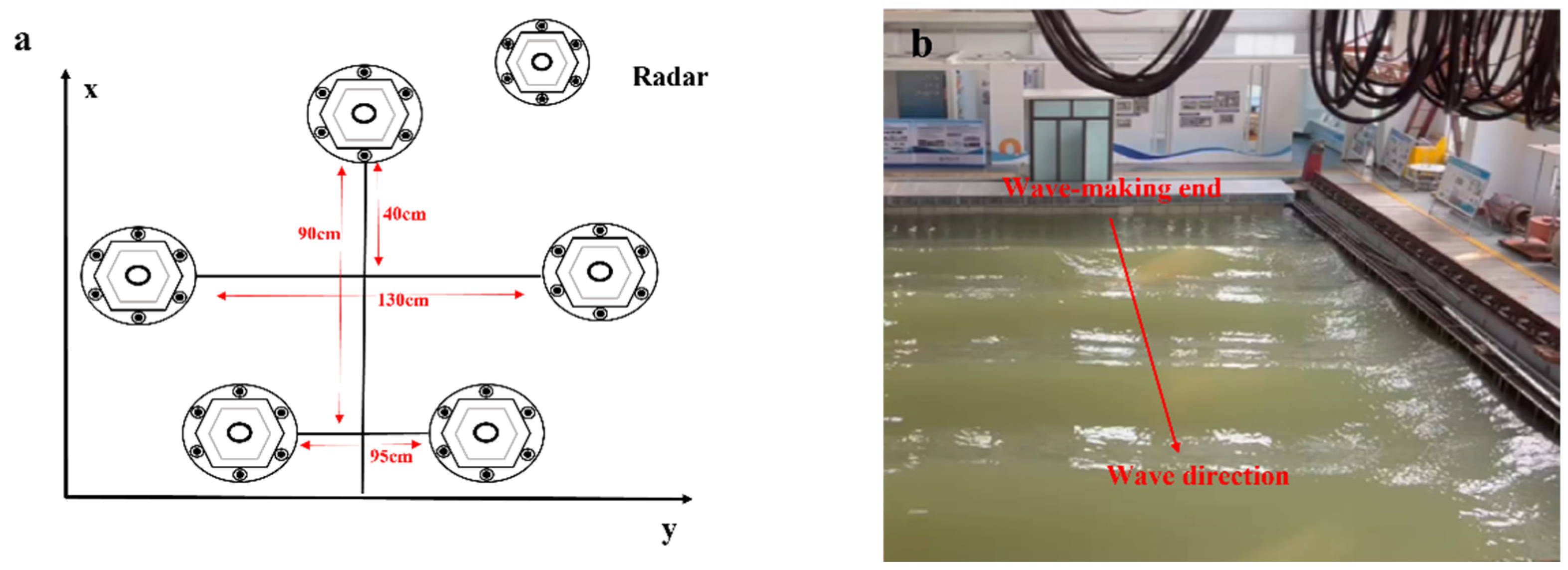
An array consisting of at least three instruments can be used to measure the wave direction. A millimeter-wave radar array was deployed on a fixed T-shaped rigid structure on the bridge deck, with the array distributed in an isosceles triangle configuration, as shown in Figure 15. According to spatial sampling theory, radars spaced 3 m apart cannot accurately capture waves with wavelengths below 3 m. Therefore, in order to correctly measure high-frequency waves, the array size should not be too large. The plane of the millimeter-wave radar array was positioned parallel to the sea surface, and its emitted electromagnetic waves incident vertically onto the sea surface, resulting in the strongest reflection intensity. The millimeter-wave radar array recorded the vertical distance to the sea surface, and the wave spectrum was obtained using the periodogram method, while the wave direction spectrum was obtained using the BDM method. The measured wave direction spectrum was compared with the actual conditions.
Figure 16a shows the distribution of the millimeter-wave radar array, and Figure 16b shows the actual propagation direction of the waves in the field. The direction was defined such that northward corresponded to 0°, and waves propagating eastward corresponded to 90°. Figure 16c represents the wave direction spectrum of the millimeter-wave radar array measurements, while Figure 16d displays the polar coordinate form of the measured wave direction spectrum. It can be observed that the direction distribution was primarily in the northeast direction, with the peak energy located at approximately 15° east of north, consistent with the actual wave direction. The measured marine area is located in the nearshore region, where in addition to waves propagating from the ocean toward the coast, waves are reflected from the coastline into the sea. The irregularities in the nearshore seabed topography and coastline can influence the propagation direction of the waves, resulting in variations and uncertainties in wave direction. In addition, the interaction between waves in the nearshore region can lead to phenomena such as wave reflection and interference, further increasing the complexity of the wave direction.
5. Conclusions and Discussion
This study utilized millimeter-wave radars to observe ocean wave heights. The reliability of using millimeter-wave radars for wave observations was preliminarily demonstrated via experiments conducted in a planar random-wave wave–current coupling pool and in an offshore environment. Compared with the capacitive wave height meter, the pulse emitted by the millimeter-wave radar illuminates a footprint, and its spectral resolution is slightly lower than the capacitive wave height meter in the high-frequency range above 2 Hz. The spectral amplitudes obtained from the millimeter-wave radar and the capacitive wave height meter measurements were not identical, and the millimeter-wave radars exhibited higher background noise in the high-frequency range. Compared with the measurements using the capacitive wave height meter, the mean bias of the measured significant wave height with the millimeter-wave radar was within the centimeter range, and the mean bias of the significant wave period was within the millisecond range. Compared with the mature commercial WG5-HT-CP radar, the spectra measured with the millimeter-wave radars were consistent in terms of peak position and magnitude. The standard deviation of the measured significant wave height between the WG5-HT-CP and the millimeter-wave radars was 0.019 m, the root mean square error was 0.026 m, and the standard deviation was 0.022 m, all within the centimeter range. The standard deviation, root mean square error, and mean bias of the wave period were all within the range of 0.210–0.329 s, which is very close to the wave period measured with the WG5-HT-CP.
The wave direction measurement experiments in the planar random-wave wave–current coupling pool showed that the wave direction retrieved with the millimeter-wave radars was consistent with the actual wave direction distribution. In the offshore field tests, due to the experimental location being in the nearshore area, the waves were influenced by the seabed topography and coastline, making the wave direction and propagation path more complex. Due to the influences of the waves coming from the offshore area, the waves reflected by the dykes on the northwest coast, and the seabed topography, the waves propagated in the direction of approximately 15°. In the ocean wave direction spectrum, there was a larger directional spread, unlike the concentrated directions obtained in the laboratory tank experiments. Since the experiment in this study was conducted in the wave tank and the offshore sea area, the significant wave heights measured in the experiments were all less than 1 m, and a test in the conditions of large wave heights was lacking, which will be the content of further comparison and discussion.
Author Contributions
Conceptualization: X.L. and Y.W.; methodology: X.L., Y.W., F.L. and Y.Z.; validation: Y.W., F.L. and Y.Z.; software: X.L. and Y.W.; formal analysis: X.L. and Y.W.; investigation: X.L., Y.W. and F.L.; writing—original draft preparation: X.L.; writing—review and editing, X.L. and Y.W.; funding acquisition: Y.W. and F.L. All authors have read and agreed to the published version of the manuscript.
Funding
This research was funded by the National Natural Science Foundation Project, grant number U22A20243; the National Outstanding Youth Science Fund Project of the National Natural Science Foundation of China, grant number 52125106; the National Natural Science Foundation of China, grant number 41976167; and the Laoshan Laboratory Science and Technology Innovation Projects, grant number LSKJ202201302.
Data Availability Statement
The data presented in this study are available on request from the corresponding author. The data are not publicly available due to privacy.
Conflicts of Interest
The authors declare no conflict of interest.
References
- Carrasco, R.; Horstmann, J.; Seemann, J. Significant wave height measured by coherent X-band radar. IEEE Trans. Geosci. Remote Sens. 2017, 55, 5355–5365. [Google Scholar] [CrossRef]
- Zeng, Y.; Song, C.; Xu, Z. Wave height estimation based on the phase time series of millimeter-wave radar. IEEE Geosci. Remote Sens. Lett. 2022, 19, 1–5. [Google Scholar] [CrossRef]
- Cavaleri, L. Wave measurement using pressure transducer. Oceanol. Acta 1980, 3, 339–346. [Google Scholar]
- Liu, Q.; Lewis, T.; Zhang, Y.; Sheng, W. Performance assessment of wave measurements of wave buoys. Int. J. Mar. Energy 2015, 12, 63–76. [Google Scholar] [CrossRef]
- Allender, J.; Audunson, T.; Barstow, S.; Bjerken, S.; Krogstad, H.; Steinbakke, P.; Vartdal, L.; Borgman, L.; Graham, C. The WADIC project: A comprehensive field evaluation of directional wave instrumentation. Ocean Eng. 1989, 16, 505–536. [Google Scholar] [CrossRef]
- Benetazzo, A. Measurements of short water waves using stereo matched image sequences. Coast. Eng. 2006, 53, 1013–1032. [Google Scholar] [CrossRef]
- Wang, J.; Hou, G.L.; Liu, Y.; Jiang, H.L. Research on shipboard wave measurement instrument based on laser technology. Ocean. Technol. 2004, 23, 14–17. (In Chinese) [Google Scholar]
- Iovescu, C.; Rao, S. The fundamentals of millimeter wave sensors. Tex. Instrum. 2017, 1–8. Available online: https://www.ti.com/lit/pdf/spyy005 (accessed on 28 September 2023).
- Marcus, M.; Pattan, B. Millimeter wave propagation: Spectrum management implications. IEEE Microw. Mag. 2005, 6, 54–62. [Google Scholar] [CrossRef]
- Wang, X.; Kong, L.; Kong, F.; Qiu, F.; Xia, M.; Arnon, S.; Chen, G. Millimeter wave communication: A comprehensive survey. IEEE Commun. Surv. Tutor. 2018, 20, 1616–1653. [Google Scholar] [CrossRef]
- Vavriv, D.M.; Bezvesilniy, O.; Volkov, V.; Kravtsov, A.; Bulakh, E. Recent advances in millimeter-wave radars. In Proceedings of the 2015 International Conference on Antenna Theory and Techniques (ICATT), Kharkiv, Ukraine, 21–24 April 2015; pp. 1–6. [Google Scholar]
- Wu, X.; Zhang, N.; Zhang, H.; Hong, W. Frequency estimation algorithm for ranging of millimeter wave LFMCW radar. In Proceedings of the 2016 IEEE International Conference on Ubiquitous Wireless Broadband (ICUWB), Nanjing, China, 16–19 October 2016; pp. 1–3. [Google Scholar]
- Stove, A.G. Linear FMCW radar techniques. IEE Proc. F (Radar Signal Process) 1992, 139, 343–350. [Google Scholar] [CrossRef]
- Beasley, P.; Stove, A.; Reits, B.; As, B. Solving the problems of a single antenna frequency modulated CW radar. In Proceedings of the IEEE International Conference on Radar, Arlington, VA, USA, 7–10 May 1990; pp. 391–395. [Google Scholar]
- Hymans, A.J.; Lait, J. Analysis of a frequency-modulated continuous-wave ranging system. Proc. IEE-Part B Electron. Commun. Eng. 1960, 107, 365–372. [Google Scholar] [CrossRef]
- Jaeschke, T.; Vogt, M.; Baer, C.; Bredendiek, C.; Pohl, N. Improvements in distance measurement and SAR-imaging applications by using ultra-high resolution mm-wave FMCW radar systems. In Proceedings of the 2012 IEEE/MTT-S International Microwave Symposium Digest, Montreal, QC, Canada, 17–22 June 2012; pp. 1–3. [Google Scholar]
- Musch, T. A high precision 24-GHz FMCW radar based on a fractional-N ramp-PLL. IEEE Trans. Instrum. Meas. 2003, 52, 324–327. [Google Scholar] [CrossRef]
- Stelzer, A.; Diskus, C.G.; Lubke, K.; Thim, H.W. A microwave position sensor with submillimeter accuracy. IEEE Trans. Microw. Theory Tech. 1999, 47, 2621–2624. [Google Scholar] [CrossRef]
- Stelzer, A.; Diskus, C.; Weigel, R. Accuracy considerations and FMCW operation of a six-port device. In Proceedings of the APMC 2001. 2001 Asia-Pacific Microwave Conference (Cat. No. 01TH8577), Taipei, Taiwan, 3–6 December 2001; pp. 407–410. [Google Scholar]
- Zech, C.; Hülsmann, A.; Schlechtweg, M.; Reinold, S.; Giers, C.; Kleiner, B.; Georgi, L.; Kahle, R.; Becker, K.-F.; Ambacher, O. A compact W-band LFMCW radar module with high accuracy and integrated signal processing. In Proceedings of the 2015 European Microwave Conference (EuMC), Paris, France, 7–10 September 2015; pp. 554–557. [Google Scholar]
- Ayhan, S.; Thomas, S.; Kong, N.; Scherr, S.; Pauli, M.; Jaeschke, T.; Wulfsberg, J.; Pohl, N.; Zwick, T. Millimeter-wave radar distance measurements in micro machining. In Proceedings of the 2015 IEEE Topical Conference on Wireless Sensors and Sensor Networks (WiSNet), San Diego, CA, USA, 25–28 January 2015; pp. 65–68. [Google Scholar]
- Ayhan, S.; Scherr, S.; Pahl, P.; Kayser, T.; Pauli, M.; Zwick, T. High-accuracy range detection radar sensor for hydraulic cylinders. IEEE Sens. J. 2013, 14, 734–746. [Google Scholar] [CrossRef]
- Jaeschke, T.; Bredendiek, C.; Küppers, S.; Pohl, N. High-precision D-band FMCW-radar sensor based on a wideband SiGe-transceiver MMIC. IEEE Trans. Microw. Theory Tech. 2014, 62, 3582–3597. [Google Scholar] [CrossRef]
- Thomas, S.; Bredendiek, C.; Pohl, N. A SiGe-based 240-GHz FMCW radar system for high-resolution measurements. IEEE Trans. Microw. Theory Tech. 2019, 67, 4599–4609. [Google Scholar] [CrossRef]
- Bhutani, A.; Marahrens, S.; Gehringer, M.; Göttel, B.; Pauli, M.; Zwick, T. The Role of Millimeter-Waves in the Distance Measurement Accuracy of an FMCW Radar Sensor. Sensors 2019, 19, 3938. [Google Scholar] [CrossRef] [PubMed]
- Mahafza, B.R. Radar Signal Analysis and Processing Using MATLAB, 3rd ed.; CRC Press: Boca Raton, FL, USA, 2016; pp. 22–24. [Google Scholar]
- Du, L.; Li, C.; Yin, G.; Lin, S. Wave monitoring array radar based on artificial intelligence algorithm. Mod. Radar 2022, 44, 41–48. [Google Scholar]
- Pierson, W.J.; Marks, W. The power spectrum analysis of ocean-wave records. Eos Trans. Am. Geophys. Union 1952, 33, 834–844. [Google Scholar]
- Blackman, R.B.; Tukey, J.W. The measurement of power spectra from the point of view of communications engineering—Part I. Bell Syst. Tech. J. 1958, 37, 185–282. [Google Scholar] [CrossRef]
- Fan, S. The evaluating method of wave power spectral density function with fast Fourier transform. Trans. Oceanol. Limnol. 1979, 2, 6–11. [Google Scholar]
- Barber, N.F. The directional resolving power of an array of wave detectors. Ocean Wave Spectra 1963, 357. [Google Scholar]
- Isobe, M.; Kondo, K.; Horikawa, K. Extension of MLM for estimating directional wave spectrum. In Symposium on Description and Modelling of Directional Seas; DHI and MMI, Copenhagen Publisher: Copenhagen, Denmark, 1984; pp. 1–15. [Google Scholar]
- Oltman-Shay, J.; Guza, R. A data-adaptive ocean wave directional-spectrum estimator for pitch and roll type measurements. J. Phys. Oceanogr. 1984, 14, 1800–1810. [Google Scholar] [CrossRef]
- Hashimoto, N.; Nagai, T.; Asai, T. Extension of the maximum entropy principle method for directional wave spectrum estimation. In Proceedings of the Coastal Engineering 1994, Kobe, Japan, 23–28 October 1994; pp. 232–246. [Google Scholar]
- Hashimoto, N. Estimation of directional spectrum using the Bayesian approach, and its application to field data analysis. Rept. PHRI 1987, 26, 57–100. [Google Scholar]
- Zhao, D.; Guan, C.; Wu, K.; Wen, S. Comparisons on estimating method of directional spectrum. Haiyang Xuebao 1999, 21, 119–125. [Google Scholar]
- Xu, D.; Yu, D. Random Wave Theory (Chinese); Higher Education Press: Beijing, China, 2001; pp. 255–256. [Google Scholar]
- Akaike, H. Likelihood and the Bayes Procedure; Springer: Berlin/Heidelberg, Germany, 1998. [Google Scholar]
- Borgman, L.E. Directional wave spectra from wave sensors. In Ocean Wave Climate; Springer: Berlin/Heidelberg, Germany, 1979; pp. 269–300. [Google Scholar]
- Rice, S. Mathematical analysis of random noise. Bell Syst. Tech. J. 1944, 23, 282–332. [Google Scholar] [CrossRef]
- Longuet-Higgins Selwyn, M. The statistical analysis of a random, moving surface. Philosophical Transactions of the Royal Society of London. Ser. A Math. Phys. Sci. 1957, 249, 321–387. [Google Scholar]
Figure 1.
The single-chirp linear-frequency-modulated continuous-wave signal and its parameters.

Figure 2.
The millimeter-wave radar water surface echoes are depicted in multiple-chirp one-dimensional range profile (a) and single-chirp one-dimensional range profile (b).
Figure 2.
The millimeter-wave radar water surface echoes are depicted in multiple-chirp one-dimensional range profile (a) and single-chirp one-dimensional range profile (b).

Figure 3.
When the radar is located on a metal platform: the occurrence of multiple reflections in wave measurements (a) and the spectrum of single-chirp signal (b).
Figure 3.
When the radar is located on a metal platform: the occurrence of multiple reflections in wave measurements (a) and the spectrum of single-chirp signal (b).

Figure 4.
The experimental measurement sites were Rainbow Bridge (a) located in the Nan District of Qingdao City, and the planar random-wave wave–current coupling pool (b) located in the Laoshan Campus of the Ocean University of China.
Figure 4.
The experimental measurement sites were Rainbow Bridge (a) located in the Nan District of Qingdao City, and the planar random-wave wave–current coupling pool (b) located in the Laoshan Campus of the Ocean University of China.

Figure 5.
The capacitive wave height meter (a) and its high-speed data acquisition system (b).

Figure 6.
Comparison of wave height time series between millimeter-wave radars and capacitive wave height meter: regular wave (a) and irregular wave (b).
Figure 6.
Comparison of wave height time series between millimeter-wave radars and capacitive wave height meter: regular wave (a) and irregular wave (b).

Figure 7.
The wave spectrum comparisons between millimeter-wave radars and the capacitive wave height meter in a planar random-wave wave–current coupling pool for regular waves (a) and irregular waves (b).
Figure 7.
The wave spectrum comparisons between millimeter-wave radars and the capacitive wave height meter in a planar random-wave wave–current coupling pool for regular waves (a) and irregular waves (b).

Figure 8.
In the case of regular waves, the arrangement of the millimeter-wave radar array (a) and the wave direction at the field (b).
Figure 8.
In the case of regular waves, the arrangement of the millimeter-wave radar array (a) and the wave direction at the field (b).

Figure 9.
In the case of irregular waves, the arrangement of the millimeter-wave radar array (a) and the wave direction at the field (b).
Figure 9.
In the case of irregular waves, the arrangement of the millimeter-wave radar array (a) and the wave direction at the field (b).

Figure 10.
Under regular wave conditions, the millimeter-wave radar array provided measurements of the wave direction spectrum in both polar form (a) and Cartesian form (b).
Figure 10.
Under regular wave conditions, the millimeter-wave radar array provided measurements of the wave direction spectrum in both polar form (a) and Cartesian form (b).

Figure 11.
Under irregular wave conditions, the millimeter-wave radar array provided measurements of the wave direction spectrum in polar form (a) and Cartesian form (b).
Figure 11.
Under irregular wave conditions, the millimeter-wave radar array provided measurements of the wave direction spectrum in polar form (a) and Cartesian form (b).

Figure 12.
Millimeter-wave radar (Left 1) and WG5-HT-CP (Left 2) field setup.

Figure 13.
The spectra (a) calculated from 20 min observation data of millimeter-wave radar and WG5-HT-CP radar, and the spectral ratio (b) between the two.
Figure 13.
The spectra (a) calculated from 20 min observation data of millimeter-wave radar and WG5-HT-CP radar, and the spectral ratio (b) between the two.

Figure 14.
The scatter plots depict wave parameters measured with the millimeter-wave radar and WG5-HT-CP radar, which include significant wave height (a), spectrum peak period (b), mean wave period (c), and mean zero-crossing wave period (d). Each scatter plot of these wave parameters comprises 53 data points, calculated at 2-min intervals.

Figure 15.
Arrangement of millimeter-wave radar array for marine field experiment.

Figure 16.
The mm wave radar array arrangement (a), the actual ocean wave (b), the rectangular coordinate (c), and the polar coordinate (d) of the wave direction spectrum measured in the field ocean experiment.
Figure 16.
The mm wave radar array arrangement (a), the actual ocean wave (b), the rectangular coordinate (c), and the polar coordinate (d) of the wave direction spectrum measured in the field ocean experiment.


Table 1.
Parameters of millimeter-wave radars.
| The Chirp Parameters | |
|---|---|
| Frequency start/GHz | 77 |
| chirp duration/ | 114.4 |
| ADC samples | 512 |
| Chirp slope (MHz/) | 10 |
| Sample rate/KHz | 5000 |
| RF gain target/dB | 48 |
Table 2.
Technical specifications.
| Working Parameters | Millimeter-Wave Radar | WG5-HT-CP |
|---|---|---|
| Frequency/GHZ | 76–81 | 9.319–9.831 |
| Modulation | LFMCW | Triangular FMCW |
| Half-power beamwidth/° | 3.5 | 5 |
| Sampling rate/HZ | 20 | 10 |
| Measuring range/m | 1–68 | 0–60 |
| Accuracy level/cm | <1 | <1 |
Table 3.
Wave parameters measured for planar random-wave wave–current coupling pool.
| Wave Parameters | Re013 | Re014 | Irre003 | Irre004 | Irre006 |
|---|---|---|---|---|---|
| SWH/m | 0.17 | 0.19 | 0.04 | 0.08 | 0.08 |
| Tp/s | 2 | 2 | 1.6 | 1.6 | 2 |
| Wave direction/° | 90 | 90 | 90 | 90 | 90 |
Table 4.
Wave parameters measured with capacitance wave meter.
| Capacitance Wavemeter Parameters | Re013 | Re014 | Irre003 | Irre004 | Irre006 |
|---|---|---|---|---|---|
| SWH/m | 0.174 | 0.205 | 0.035 | 0.073 | 0.076 |
| Tp/s | 1.985 | 1.985 | 1.724 | 1.724 | 2.059 |
Table 5.
Wave parameters measured with millimeter-wave radars.
| Radar Parameters | Re013 | Re014 | Irre003 | Irre004 | Irre006 |
|---|---|---|---|---|---|
| SWH/m | 0.153 | 0.176 | 0.034 | 0.084 | 0.064 |
| Tp/s | 1.985 | 1.985 | 1.699 | 1.699 | 2.059 |
| BIAS | BIAS | ||||
| SWH/m | 0.025 | 0.008 | |||
| Tp/s | 0 | 0.017 | |||
Table 6.
The statistical parameters of the differences between the wave parameters measured with the millimeter-wave radar and WG5-HT-CP.
Table 6.
The statistical parameters of the differences between the wave parameters measured with the millimeter-wave radar and WG5-HT-CP.
| Hm0/m | Tp/s | Tm01/s | Tm02/s | |
|---|---|---|---|---|
| STD | 0.019 | 0.291 | 0.329 | 0.227 |
| RMS | 0.026 | 0.279 | 0.312 | 0.232 |
| BIAS | 0.022 | 0.223 | 0.253 | 0.210 |
Disclaimer/Publisher’s Note: The statements, opinions and data contained in all publications are solely those of the individual author(s) and contributor(s) and not of MDPI and/or the editor(s). MDPI and/or the editor(s) disclaim responsibility for any injury to people or property resulting from any ideas, methods, instructions or products referred to in the content. |
© 2023 by the authors. Licensee MDPI, Basel, Switzerland. This article is an open access article distributed under the terms and conditions of the Creative Commons Attribution (CC BY) license (https://creativecommons.org/licenses/by/4.0/).
Share and Cite
MDPI and ACS Style
Liu, X.; Wang, Y.; Liu, F.; Zhang, Y. Investigation on the Utilization of Millimeter-Wave Radars for Ocean Wave Monitoring. Remote Sens. 2023, 15, 5606. https://0-doi-org.brum.beds.ac.uk/10.3390/rs15235606
AMA Style
Liu X, Wang Y, Liu F, Zhang Y. Investigation on the Utilization of Millimeter-Wave Radars for Ocean Wave Monitoring. Remote Sensing. 2023; 15(23):5606. https://0-doi-org.brum.beds.ac.uk/10.3390/rs15235606
Chicago/Turabian StyleLiu, Xindi, Yunhua Wang, Fushun Liu, and Yuting Zhang. 2023. "Investigation on the Utilization of Millimeter-Wave Radars for Ocean Wave Monitoring" Remote Sensing 15, no. 23: 5606. https://0-doi-org.brum.beds.ac.uk/10.3390/rs15235606
Note that from the first issue of 2016, this journal uses article numbers instead of page numbers. See further details here.