
Planetary Radar—State-of-the-Art Review
by
 , , , , , and
Anne K. Virkki
1,2,*,
Catherine D. Neish
3,
Edgard G. Rivera-Valentín
4,
Sriram S. Bhiravarasu
5,
Dylan C. Hickson
6,
Michael C. Nolan
7 and
Roberto Orosei
8
1
Department of Physics, University of Helsinki, Gustaf Hällströmin katu 2a, 00560 Helsinki, Finland
2
Finnish Geospatial Research Institute, National Land Survey, 02150 Espoo, Finland
3
Department of Earth Sciences, University of Western Ontario, London, ON N6A 3K7, Canada
4
Johns Hopkins University Applied Physics Laboratory, Laurel, MD 20723, USA
5
Space Applications Centre, Indian Space Research Organisation, Ahmedabad 380015, India
6
MDA Geospatial Services Inc., Ottawa, ON K2E 8B2, Canada
7
Lunar and Planetary Laboratory, University of Arizona, Tucson, AZ 85721, USA
8
INAF—Istituto di Radioastronomia, 40128 Bologna, Italy
*
Author to whom correspondence should be addressed.
Remote Sens. 2023, 15(23), 5605; https://0-doi-org.brum.beds.ac.uk/10.3390/rs15235605
Submission received: 31 October 2023
/
Revised: 24 November 2023
/
Accepted: 27 November 2023
/
Published: 2 December 2023
(This article belongs to the Special Issue Radar for Planetary Exploration)
Abstract
:Planetary radar observations have provided invaluable information on the solar system through both ground-based and space-based observations. In this overview article, we summarize how radar observations have contributed in planetary science, how the radar technology as a remote-sensing method for planetary exploration and the methods to interpret the radar data have advanced in the eight decades of increasing use, where the field stands in the early 2020s, and what are the future prospects of the ground-based facilities conducting planetary radar observations and the planned spacecraft missions equipped with radar instruments. The focus of the paper is on radar as a remote-sensing technique using radar instruments in spacecraft orbiting planetary objects and in Earth-based radio telescopes, whereas ground-penetrating radar systems on landers are mentioned only briefly. The key scientific developments are focused on the search for water ice in the subsurface of the Moon, which could be an invaluable in situ resource for crewed missions, dynamical and physical characterization of near-Earth asteroids, which is also crucial for effective planetary defense, and a better understanding of planetary geology.
1. Introduction
Radar observations have been increasingly used for planetary science over the past eight decades. Radar, a term derived from “radio detection and ranging”, is a powerful tool for measuring not only the range and rotation rates of planetary objects, but also their reflective and polarimetric scattering properties at microwave wavelengths. The basic concept of the radar technique for scientific purposes is transmitting a radio signal and receiving the echo, which carries a wealth of information about the object being investigated. For example, the round-trip time of a coded radar signal can be used for an accurate range measurement. In addition, the wave properties of the received signal can be compared to the known properties of the transmitted signal to reveal information about the physical and dynamical properties of the target.
In this overview article, we highlight some of the most important advances in planetary science that were facilitated by radar remote sensing (Earth-based interplanetary and orbital observations) with a focus on the last two decades. The first extraterrestrial radar target was the Moon in 1946, but as of today, radar observations have been conducted for all terrestrial planets, the rings and several moons of Jupiter and Saturn, comets, and more than a thousand asteroids. Radar observations have been conducted using Earth-based telescopes and numerous space-based instruments. Incoherent scatter radar (ISR; see the list of abbreviations at the end of the paper) systems, such as the European Incoherent Scatter Scientific Association (EISCAT) system in the Nordic countries, Jicamarca in Peru, or the Sanya ISR in China, can observe the Moon and could also be able to observe near-Earth asteroids in certain conditions (e.g., [1,2]); however, these systems are not optimized for planetary radar observations, and would thus be unlikely to conduct many observations. Therefore, they will not be discussed in further detail.
In Section 2, we provide a brief contextual history of the major findings achieved using planetary radar and the key instruments that have been utilized. In Section 3, we describe some of the most important methods of radar observations and the methodological advancements in the last two decades that have improved the interpretation and analysis of radar data. Section 4, Section 5 and Section 6 provide an overview on the state-of-the-art radar studies of the Moon, planets and their satellites, and small Solar System objects (SSSOs), respectively, using both Earth-based and space-based observations. Finally, Section 7 gives some future prospects for radar-related technologies and instruments.
2. A Brief History of Planetary Radar
2.1. Planetary Radar Science in the 20th Century
Several planetary radar facilities became operational in the late-1950s to the early 1960s as a part of the space race between the United States and the former Soviet Union. The Goldstone Deep Space Communications Complex in California opened in 1958 and the Arecibo Observatory in Puerto Rico opened in 1963, whereas the Pluton facility in Crimea opened in 1960. The Lincoln Laboratory’s Lincoln Space Surveillance Complex, the home of the Haystack Observatory and the Millstone Hill Geospace Facility, was also a pioneering radar facility, although regular observations were focused on ionospheric observations. The Millstone Hill radar installation conducted the first radar observation of Venus in 1958 [3].
The first important results of planetary radar science focused on the Moon and the terrestrial planets. Radar observations at Arecibo using the 305-m William E. Gordon telescope in the 1960s revealed the true rotation rates of Mercury and Venus, as well as Mercury’s perihelion advance [4,5,6]. Observations of Jupiter were attempted in the 1960s but, due to its gas giant nature, Jupiter was not observable [7]. The Galilean satellites, though, were observed in 1976 after the S-band radar was added and the antenna dish was improved during a telescope upgrade [8]. In 1969, the first radar observations of asteroids were conducted, with (1566) Icarus being the first target [9,10]. In 1980, Comet 2P/Encke was observed, marking the first radar observation of a comet [11]. In addition to their rotation rates, radar provided information about the sizes of planetary objects. This fact is particularly important for comets, as the light scattered by the nucleus is often optically dominated by the light scattered by the coma.
The first space-based radar instruments were used for experiments in the 1970s. Namely, the Apollo 17 mission hosted the Lunar Radar Sounder Apollo Lunar Sounder Experiment (ALSE) as part of its scientific instrumentation. This instrument was used for transmitting pulses from lunar orbit to probe the subsurface of the Moon to a depth of about 1.3 km using high-frequency (HF) and very high frequency (VHF) bands.
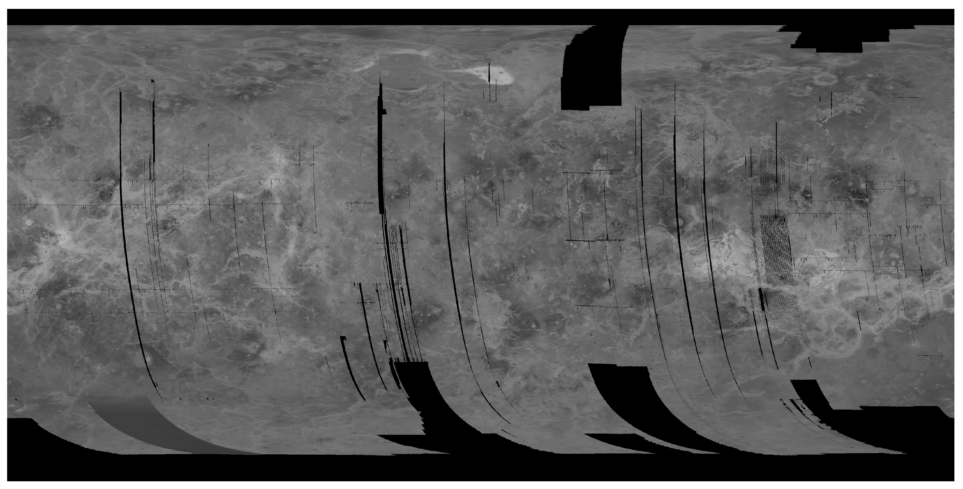
Radar remote sensing also gave us our first views of the surface of Venus. Given its thick atmosphere, that is mostly opaque at optical and infrared wavelengths, radar remote sensing is the only method capable of mapping the surface of Venus. In 1983–1984, Venera 15 and 16 mapped the surface of Venus from its north pole to a latitude of N using SAR instruments and radio altimeter systems. NASA’s Magellan mission followed six years later and mapped the surface of Venus in 1990–1994. More than 80% of the surface was mapped during cycle 1 (Figure 1), with 98% of the planet mapped by the end of the mission (e.g., [12]). While Venera used an 8 cm wavelength radar and provided a spatial resolution of 1 to 2 km, the maps made using Magellan’s 12.6 cm radar system had spatial resolutions one order of magnitude finer at 100 m.
One of the major findings in planetary radar science in the 20th century was the enhancement of the radar echo in ice. Observations of the icy Galilean moons revealed anomalously high radar reflectivity compared to radar targets whose surfaces are dominated by silicate- or carbon-rich regolith. In the 1990s, observations of the permanently shadowed regions of Mercury’s poles also revealed anomalously bright radar echoes, which were attributed to ice [13,14,15,16]. While the enhancement was understood to be due to subsurface multiple scattering, Hapke [17] and Peters [18] showed that the coherent backscattering effect was the source of the enhancement in the reflectivity, as well as unusual polarization properties. The unique radar signature of water ice has motivated years of radar observations of particularly the Moon in search of subsurface ice deposits, as it is considered a valuable in situ resource for future crewed missions.
2.2. Planetary Radar Science in the 21st Century
In the 21st century, Earth-based planetary radar observations have focused heavily on near-Earth asteroids. This is primarily due to a boost in funding related to planetary defense, which followed from the George E. Brown, Jr. Near-Earth Object Survey Act that became part of the NASA Authorization Act of 2005 (https://www.gpo.gov/fdsys/pkg/PLAW-109publ155/pdf/PLAW-109publ155.pdf, accessed on 26 November 2023). The number of known near-earth asteroids (NEAs) began to steeply increase, and consequently, the number of radar-observed asteroids increased from less than 100 by the year 2001 to more than 1000 by the year 2021. Also, the quality of the planetary radar data improved further after the S-band-transmitter and dish upgrade at Arecibo in the 1990s that allowed even better signal-to-noise ratios for smaller and/or farther targets.
The range and Doppler information of nearly 1000 NEAs from radar observations has improved the available orbital information of these objects [19,20]. This is a crucial part of planetary defense in terms of evaluating the risks that the NEAs pose. The most prominent example is (99942) Apophis, which will pass by the Earth at less than 40,000 km above the Earth’s surface on the 13 April 2029. When Apophis was discovered in 2005, planetary radar observations were key to determining the risk that this 340-m asteroid poses, as its impact could decimate a small country [21,22]. As the number of asteroid observations increased, planetary radar observations were also able to reveal the diversity of the physical characteristics of asteroids. Radar observations of asteroids have continued to be crucial for space missions to these worlds, as radar imaging provides more direct data on the topographic features of the targets than visual and near-infrared (VNIR) observations (e.g., [23,24]). The variance in the observed radar reflectivity is indicative of the near-surface density and the abundance of metals, (e.g., [25,26,27]), and the polarimetric properties provide clues to the surface texture at the decimeter scale (see Section 3.6). Also, radar data were used to directly observe the change in the rotation rate of an asteroid for the first time [28]. The asteroid and comet radar observations are discussed in more detail in Section 6.
The continued Earth-based observations of Mercury, Venus, and Mars have provided more coverage and finer resolutions at better signal-to-noise ratios than the observations in the 20th century had been able to provide, which has allowed for, e.g., better geological characterization of craters, lava flows, ice deposits, and other intriguing features (e.g., [16,29,30,31]). The findings for each planet and a summary table are described in further detail in Section 5.
Furthermore, the space-based radar observations have taken a long leap forward in the 21st century. For example, the orbital sounding radars Mars Advanced Radar for Subsurface and Ionosphere Sounding (MARSIS), which began science operations in 2005, and Mars SHAllow RADar sounder (SHARAD), operational since 2006, have helped to characterize the subsurface geology and to quantify the volatiles inventory on Mars (e.g., [32,33]). Radar signals using low frequencies are able to penetrate deep into the subsurface. MARSIS uses transmission frequencies as low as 1.8–5.0 MHz, whereas SHARAD has a carrier frequency of 20 MHz [34], which has allowed MARSIS to detect echoes from as deep as 3.7 km [35], whereas SHARAD provides a finer vertical resolution, 15 m or less depending on the material being sounded [34].
The 21st century brought new observations of Titan and the Moon by orbital radar systems as well. Cassini Ku-band (13.8 GHz, 2.2 cm) radar observations revealed the first high-resolution views of Titan’s surface in the mid-2000s, including large methane lakes near its poles [36]. Japan’s Selenological and Engineering Explorer (SELENE) spacecraft observed the Moon using the Lunar Radar Sounder (LRS; with a center frequency of 5 MHz) in 2007–2009. We have also obtained global views of the Moon with the Miniature Radio-Frequency (Mini-RF) instrument on the Lunar Reconnaissance Orbiter (LRO), launched in 2009. It was built as a technology demonstration of a lightweight dual-frequency synthetic aperture radar (DFSAR), in contrast to the heavy radar systems of the 20th century [37]. The Mini-RF system has two separate bands, one at 12.6 cm and one at 4.2 cm, and is able to image the lunar surface at a 30 m resolution. It was originally able to transmit, but since 2011 observations have been bistatic, with Arecibo or Goldstone transmitting and Mini-RF receiving. LRO provided the first observations of the lunar far side and the first complete map of the lunar poles at radar wavelengths [38]. The science mission of Mini-RF has been primarily to search for water ice near the poles and characterize the geology of the Moon (see Section 4 for further details on the findings). Lunar orbital radar observations were also conducted by the S-band radar on Chandrayaan-1 in 2008–2009 during its one year of operations before the loss of communication, and DFSAR on Chandrayaan-2, launched in 2019, which provided the first L-band radar observations of the Moon [39].
In terms of recent changes in the Earth-based radar observation capabilities, the Canberra radar began asteroid observations in 2015 and has since observed up to eight asteroids per year (https://echo.jpl.nasa.gov/asteroids/PDS.asteroid.radar.history.html, accessed on 26 November 2023). The Arecibo radar became nonoperational in 2020 after two cable failures led to the collapse of the telescope. Consequently, the radar observations of other planets and a large number of asteroids have become significantly more challenging with the current radar infrastructure due to the lower available transmission power and smaller antenna sizes. The Goldstone Solar System Radar and Canberra radar are currently the only facilities that have conducted several asteroid observations over the last year. Recently, some European facilities have also been participating in individual bistatic radar observations of asteroids with a transmission using DSS-63 in Spain or DSS-14 at Goldstone, and a reception using radio telescopes in Italy (Sardinia, Medicina, and Noto) and Germany (Effelsberg) (e.g., [40,41]), and a new radar array facility is being built in Chongqing, China. Green Bank Observatory has plans for a new radar system as well; the first observation experiments of a low-power transmission have already been conducted [42]. See Section 7 for more details on future radar facilities.
3. Methods Used in Radar Studies
3.1. Echo Power Spectra
In a typical planetary radar observation, a high-power microwave signal is transmitted at a specified target, and the echo of the signal is received using the same telescope in a monostatic observation or a different telescope in a bistatic observation. In a monostatic observation, the transmission for each “scan” lasts through one round-trip time of the signal, e.g., for one minute for a target that is 30 light-seconds away minus the time required for switching from the transmission to receiving mode or vice versa. This timing allows for switching between the transmission and receiving in a way that optimizes the used power, where the system is switched to receiving right before the echo of the beginning of the scan is to return, and switched back to transmission after the whole echo of the scan has been received.
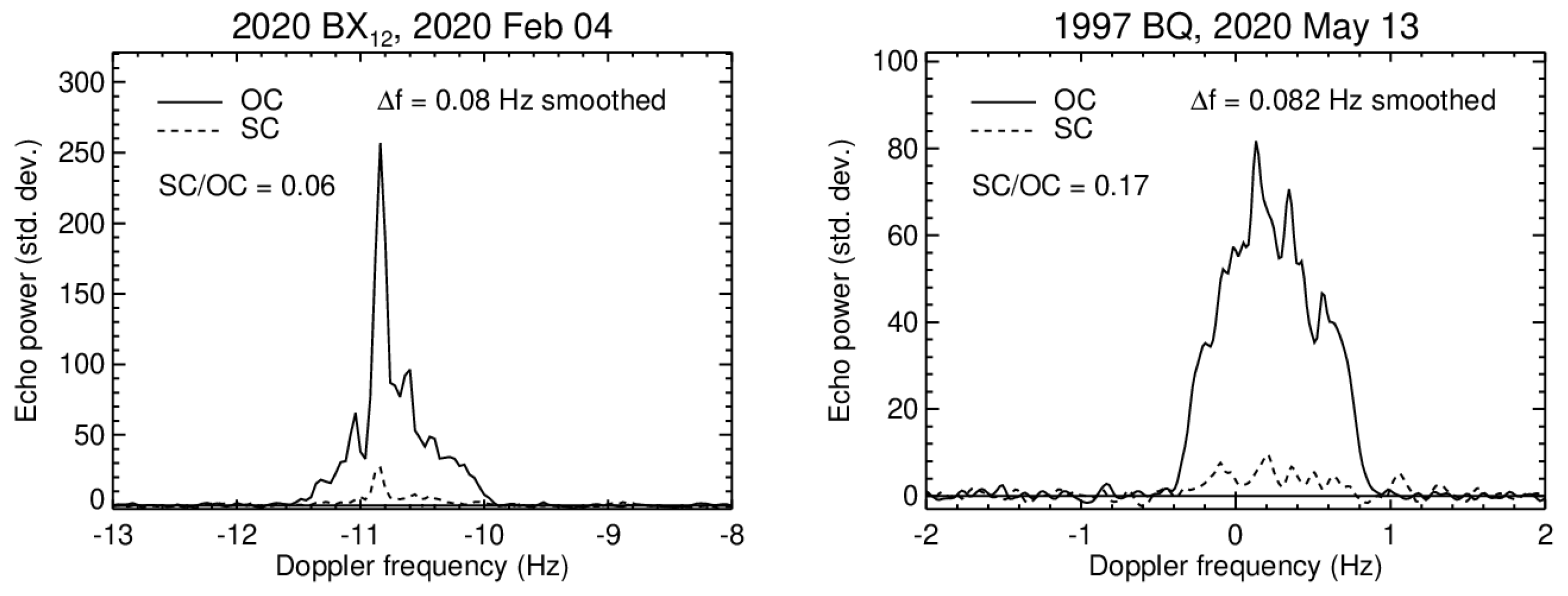
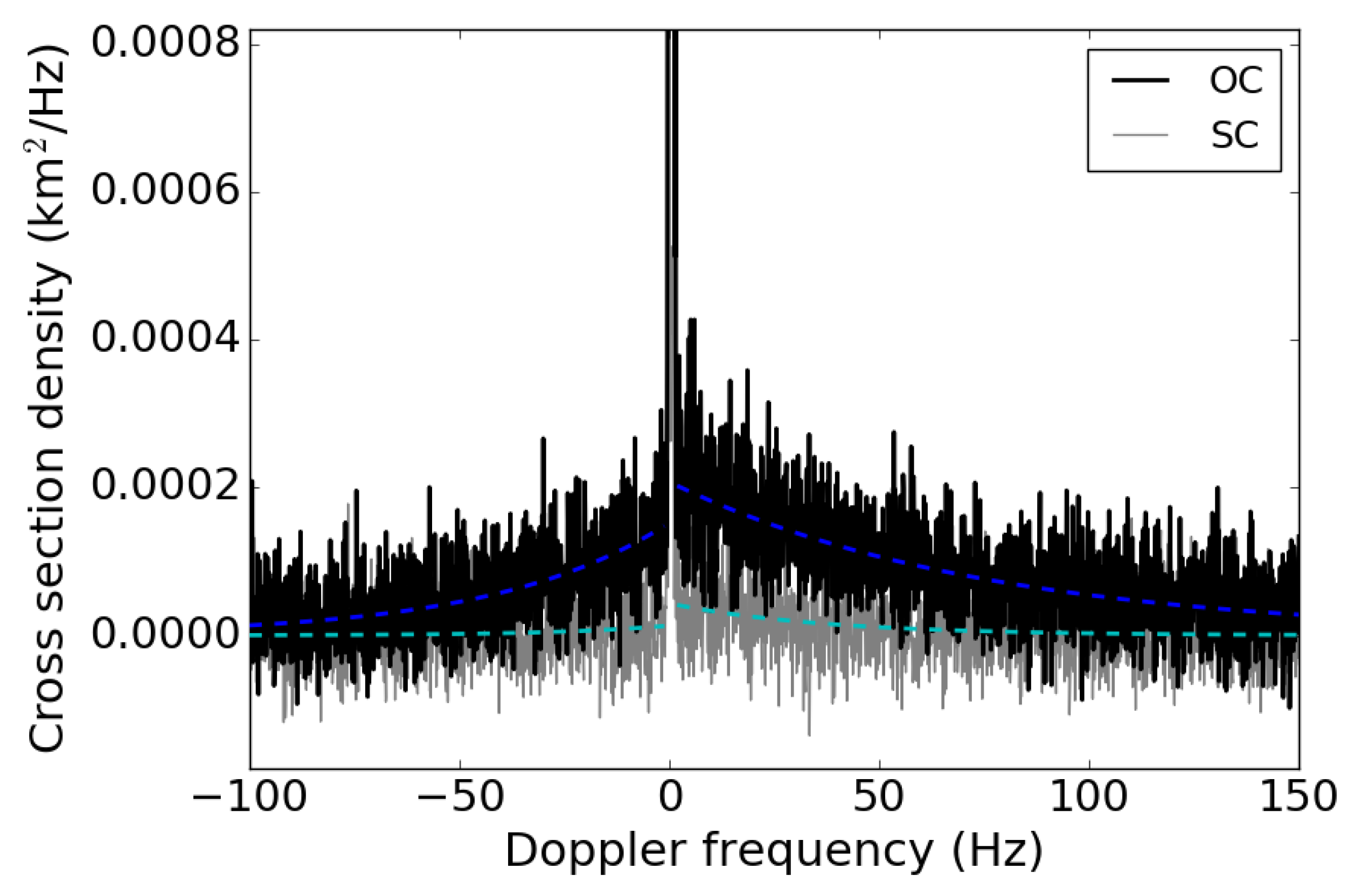
The ephemeris for a target (i.e., its position in space) is required to provide its plane-of-sky location to an accuracy of half the beam width of the transmitting radar. The ephemeris also provides an estimate of the range and an expected Doppler shift. The Doppler echo power spectrum records the echo power as a function of the Doppler shift. The processing is typically performed with respect to the expected Doppler shift and the noise-power level, so that the origin of the spectrum is set at the expected Doppler shift at horizontal zero, and the mean of the Gaussian-distributed noise-power level is at the vertical zero (see Figure 2). The integration of the received echo power with proper normalization provides the radar cross-section (typically denoted as ), which is descriptive of the total radar reflectivity of the target. The expected received power can be estimated using the radar equation:
where is the transmitted power, is the wavelength, and are the antenna gains, respectively, for transmission and reception (or equivalently, times the effective aperture of the antenna), and and are the target’s distance, respectively, from the transmitter and the receiver. For Earth-based observations of planetary objects, even for bistatic observations, whereas for a space-based observation the two distances could be significantly different. The received signal’s polarization information may also be recorded, as is described in detail in Section 3.6. In Figure 2, two senses of circular polarizations are included: same-circular (SC) polarization and opposite-circular (OC) polarization with respect to the transmitted signal, as well as the ratio of the radar cross-sections in the SC polarization to that in the OC polarization, i.e., the circular polarization ratio (CPR or SC/OC ratio).
More specifically, the echo power per Doppler shift bin is normalized by one echo power standard deviation (z-score in statistics), which is essentially the signal-to-noise ratio (S/N). Virkki et al. [43] define the z-score per frequency bin as
where is the partial radar cross-section that falls under the frequency bin, is the Boltzmann constant, is the receiver’s system temperature [44], is the Doppler frequency resolution determined by the fast Fourier transform length applied to obtain the spectrum, and is the number of looks, i.e., independent estimates of , which is related to the scan (or integration) time, , and the frequency resolution, so that . The frequency resolutions for long scans can thus be finer than mm/s. Integration over several frequency bins is often required to obtain a z-score that is useful for further analysis.
The echo power spectra can be used for estimating the target’s spin period (P), diameter (D) projected on the plane of sky), or the subradar latitude () based on the Doppler bandwidth (B):
Due to the ambiguity of the period, diameter, and the subradar latitude, two must be known to derive the third. If only the period is known, a lower limit of the diameter can be determined by assuming an equatorial view as . Optionally, if only the diameter is known, an upper limit can be set for the period.
If the target’s projected area () can be estimated based on the radar observations or observations at other wavelengths, the radar cross -ection can be used for estimating the radar albedo:
The radar albedo can be polarization-specific or the total albedo for all polarizations. In the literature, the radar albedos of asteroids are typically reported in the OC polarization, but some exceptions occur. It is related to the backscatter coefficient, which is also an area-normalized radar cross-section, but more commonly used when the radar beam does not cover the whole target but only a part of the surface (e.g., an orbital radar illuminating a planet).
3.2. Ranging and Delay–Doppler Imaging
A delay–Doppler image is a map of the echo power in the delay–Doppler space. A measurement of the radar signal delay (round-trip time) is required for measuring range. While the Doppler echo power spectra can be generated using a continuous wave, a range measurement requires modulation of the radar signal. The modulation can be performed as binary-phase coding (BPC) or as frequency modulation (also known as chirp). The range resolution depends on the system; for example, if the BPC-modulator changes the phase at a frequency of 40 MHz (once per 0.1 s), the apparent range resolution is 15 m. See, for example, refs. [43,44,45] for more technical details, and [46] for the capabilities of NASA’s Deep Space Network (DSN) telescopes and the Arecibo legacy S-band radar.
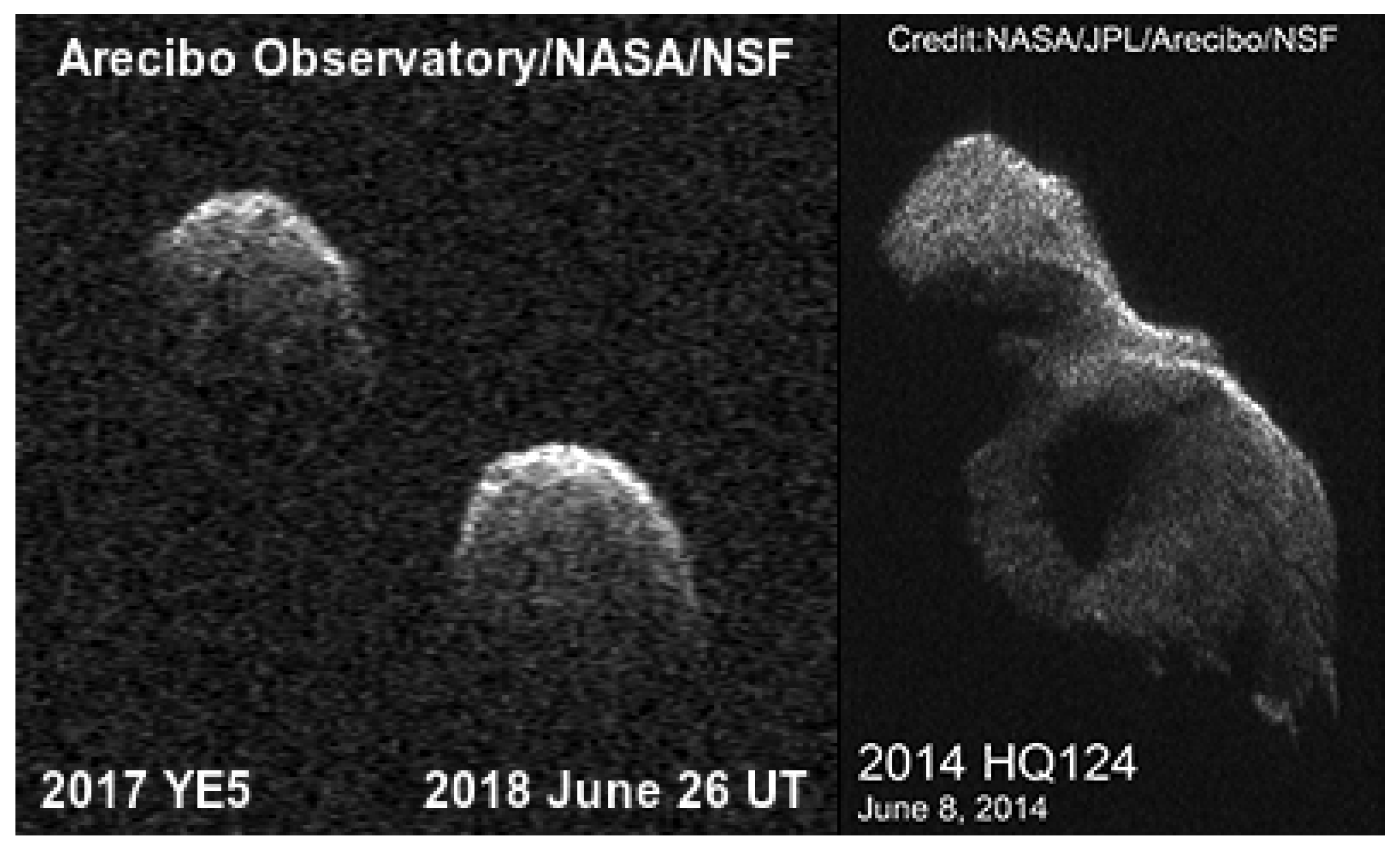
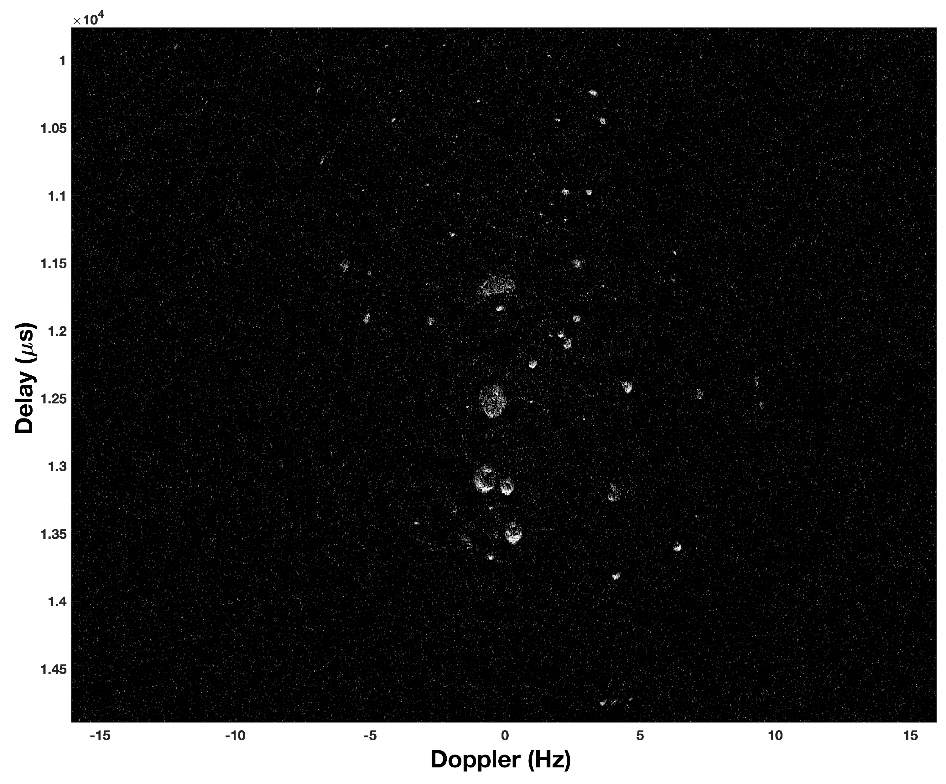
Delay–Doppler imaging allows for higher resolution maps of planetary bodies than any other ground-based imaging method, including VNIR wavelengths, and range measurements can be as precise as a few meters at best. For example, Figure 3 shows an example of delay–Doppler images of NEAs 2017 YE5 at a range resolution of 7.5 m (vertical so that the range increases from top down) and a frequency resolution of 0.0204 Hz (horizontal), and 2014 HQ124 at a range resolution of 1.875 m and a frequency resolution of 0.00625 Hz. Also, the backscatter coefficient can be plotted as a function of the incidence angle in each polarization, which can be used for scattering analysis (described in more detail in Section 3.6). Delay–Doppler imaging has been a key technique for the mapping of planets and the Moon. This is especially true for Venus, which is covered by a thick, opaque atmosphere. However, high-resolution imaging of Venus has required wavelengths of 3–5 cm or longer, as shorter wavelengths are heavily affected by atmospheric opacity [47].
3.3. Synthetic Aperture Radar
Orbital radars also acquire information in delay–Doppler space. Here, the Doppler shift is measured in the “along-track” direction, while the delay is measured in the “cross-track” direction. (These directions refer to the motion of the spacecraft orbiting above a planet’s surface.) The Doppler resolution in this case corresponds to the two nearest separable points along a constant delay line. For real-aperture radars, this is equal to the width of the antenna footprint, which is generally quite large. Synthetic-aperture radars (SARs) improve upon this resolution by taking advantage of the fact that a single point can be observed multiple times along the orbital path. These echoes acquired along a segment of the orbit can be coherently summed to synthesize a much larger antenna, which results in a much smaller beam width, and an increase in the S/N of the range line at the center of the aperture (e.g., [48]). A curious effect of this approach is that the along track resolution is independent of the altitude of the orbiting radar. This is because as the radar moves further from the surface, it will create a larger footprint on the ground, but also result in a longer synthetic array. This increases the effective resolution of the radar, since resolution is inversely proportional to the diameter of the array. Combined, the larger size of the synthetic array exactly compensates for the larger footprint size, maintaining the resolution in the azimuth (along-track) direction. High resolution in the range (cross-track) direction is achieved by transmitting very short pulse durations. To achieve short pulse durations, the “pulse compression” technique [49] is used. This technique consists of emitting high-energy pulses that are linearly modulated in frequency (“chirp”). The range resolution using a modulated pulse is a function of the chirp bandwidth and not the physical pulse length.
Most imaging SAR instruments are side-looking. Because they translate time delay into distance from the spacecraft, a nadir-pointed SAR would, therefore, translate a location to the left of the spacecraft into the same pixel as a location an equal distance to the right of the spacecraft. Pointing the SAR instrument to the side avoids any left–right ambiguity. Orbital SAR instruments have been used to successfully observe the Earth, the Moon, Venus, and Titan. Recently, experimental SAR techniques applied to ground-based radar images of the Moon have been shown to produce high-resolution imaging results [42].
3.4. Radar Sounding of Subsurface
Electromagnetic waves at frequencies in the MF, HF, and VHF portions of the radio spectrum are capable of penetrating into most natural materials up to hundreds of wavelengths, depending on the nature of the material, before being absorbed. Radar scattering properties scale with wavelength, where signals from 1 MHz to 1 GHz allow penetration in dry regolith and ice up to kilometers depth in some cases. If a dielectric discontinuity is present within the material, part of the wave is backscattered, and can be detected by a receiving antenna. This property has been used in radio echo sounding, or ice-penetrating radar, an established geophysical technique that has been used for more than five decades to investigate the structure of ice sheets and glaciers in Antarctica, Greenland, and the Arctic. Subsurface dielectric discontinuities in the form of layered sedimentary deposits or volumetric inclusions are imaged at resolutions of tens of meters to reveal complex deposition histories in ice as well as regolith formation processes. In planetary exploration, the first instrument of this kind, often called a radar sounder, was the Apollo Lunar Sounding Experiment (ALSE) on board Apollo 17 [50].
Because of the long wavelengths transmitted, instruments of this kind have to use dipoles for antennas, which have negligible directivity and, thus, spread the pulse energy in all directions. To ameliorate this problem, subsequent radar sounders employed the SAR method described above. A two-dimensional radargram is created with the range direction on the vertical axis and subsequent ranging measurements aligned in the along-track direction on the horizontal axis, with the spacing determined by the synthetic aperture chosen. The SAR focusing permits interpretation of continuous structures through the observed volume. The Mars Advanced Radar for Subsurface and Ionosphere Sounding (MARSIS) [51] and the SHAllow RADar (SHARAD) [34] were the first to utilize this technique to explore the subsurface of Mars, followed by the Lunar Radar Sounder [52] onboard the SELENE orbiter on the lunar orbit and more recently by the Mars Orbiter Subsurface Investigation Radar (MOSIR) [53], again on Mars.
Radar sounding by the MARSIS and SHARAD missions has been integral to deciphering the ancient climate of Mars by revealing properties of the polar layered ice deposits. The Lunar Radar Sounder observed reflections interpreted as originating from lava tubes on the Moon [54], and similar efforts to constrain the locations of lava tubes on Mars have also been explored [55]. Another radar experiment, the Comet Nucleus Sounding Experiment by Radiowave Transmission (CONSERT), has probed the interior of the nucleus of comet 67P/Churyumov–Gerasimenko in a bistatic configuration, in which radio waves were transmitted from an orbiter and recorded by a lander on the surface of the comet nucleus [56] (see Section 6). In the near future, the Radar for Icy Moon Exploration (RIME) [57] and the Radar for Europa Assessment and Sounding: Ocean to Near-surface (REASON) [58] will explore the icy crust of the Galilean satellites of Jupiter.
Ground-penetrating radar (GPR) instruments are similarly used for subsurface imaging by exploiting radar antenna(s) that are raised just above the ground surface on some moving platform. In the context of planetary exploration missions, robotic rovers carry these instruments to create 2D radargrams along the traversed path. While the spatial coverage of measurements is, therefore, much lower when compared with orbital SAR sounders, higher frequencies can be exploited to enable superior resolution imaging. There are several examples of GPR instruments that have been used for planetary exploration, such as the Radar Imager for Mars’ subsurface experiment (RIMFAX) GPR onboard the Perseverence rover on Mars, a GPR onboard the Yutu rover of the Chang’e 3 mission on the Moon, the Lunar Penetrating Radar (LPR) onboard the Chang’e 4 rover, and the Lunar Regolith Penetrating Radar (LRPR) onboard the Chang’e 5, also on the Moon. However, in this overview paper we focus on radar as an orbital and interplanetary remote sensing technique for planetary exploration, so GPR instruments will not be discussed in further detail.
3.5. Shape Modeling
One of the main benefits of the fine spatial resolution of delay–Doppler images is the direct information provided about the shape of the object. When the spatial resolution is much finer than the size of the object and the S/N allows, individual features can be distinguished, and in some cases the full shape of the object can be derived. The shapes of asteroids are diverse and a spherical shape is in very few cases a good approximation. Knowing the true shape can be useful in many further applications related to understanding the physical properties of the asteroid, from gravitational properties to regolith cohesion and scattering properties.
The main challenges in deriving the shape using radar images is the north–south ambiguity of the delay–Doppler imaging. Although the latitude and longitude of the spin axis can often be quite well constrained, determining the direction of the rotation is not always straightforward. The inverse modeling of the shape from the radar images requires high S/N data obtained in several rotational and plane-of-sky orientations. Lightcurves at optical wavelengths are a helpful complement; in fact, most software that has been developed for shape modeling using radar data, also include the capability to use lightcurve data as well. Two examples of such software that have been widely used for the shape modeling of SSSOs are Shape (e.g., [59]) and the All-Data Asteroid Modeling (ADAM) algorithm [60].
3.6. Radar Scattering
3.6.1. Dual-Polarization Radars
In a typical dual-polarization radar observation, the radar system transmits a high-power signal that has a fixed polarization state. The ground-based facilities (Arecibo and Goldstone) have most commonly used circular polarization, whereas space-based radar systems have often opted for linear polarization. Considering the heritage from ground-based planetary radar studies, the Mini-SAR on board Chandrayaan-1 and LRO’s Mini-RF are hybrid polarized radars, transmitting circularly polarized light and receiving echoes in both linear senses, otherwise known as compact polarimetry. The echo signal’s intensity and polarization state are coherently received in orthogonally polarized receiver channels, which allows for polarimetric analysis of the target’s near surface. Due to the penetration depth of long wavelengths, the radar echo provides information of the near surface up to several wavelengths deep depending on the target’s absorption properties; it is not necessarily limited only to the visible surface.
The backscattered field can be described using the four Stokes parameters (in the backscattering alignment convention):
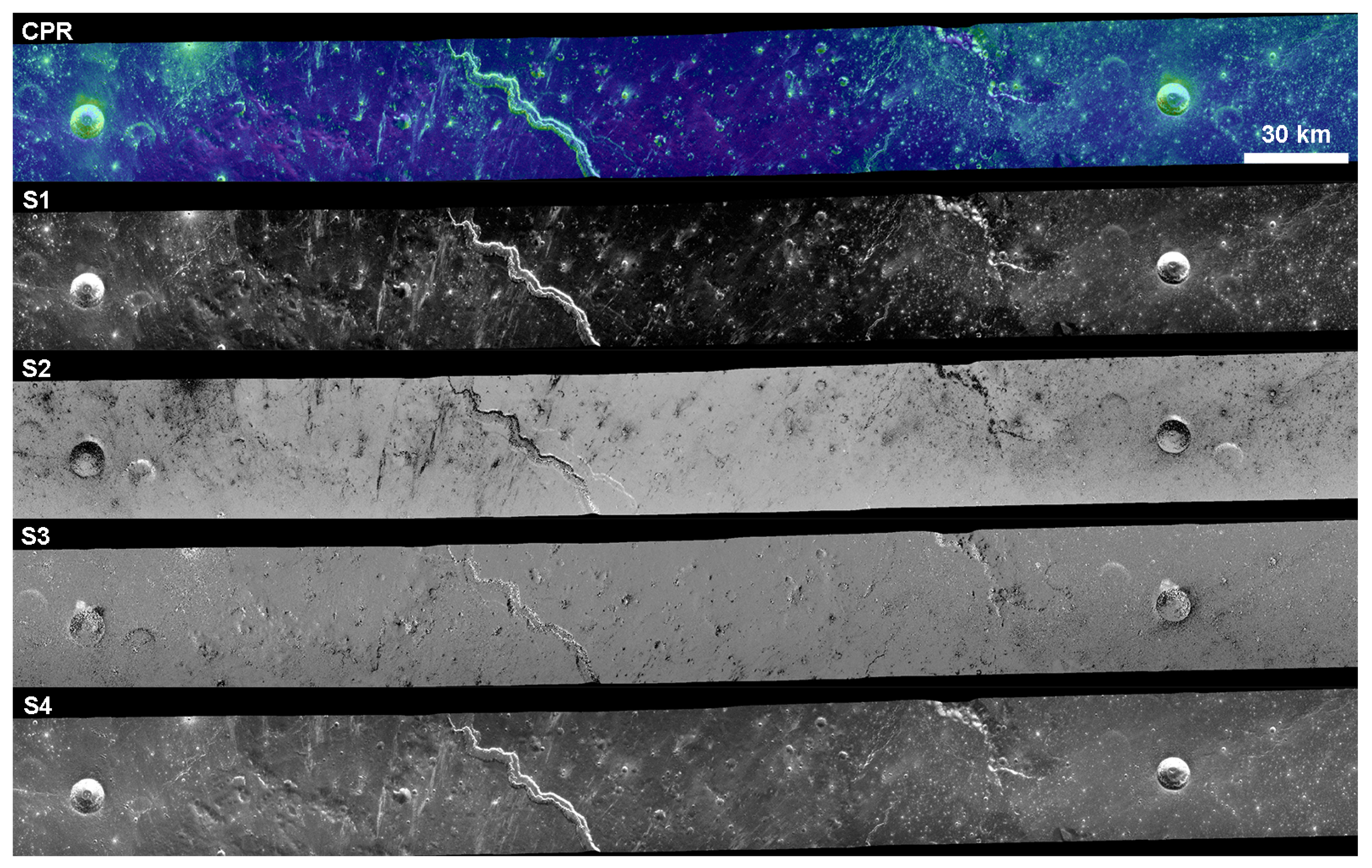
where the subscripts H and V indicate the linear horizontal and vertical polarizations, and L and R are the left- and right-handed circular polarizations, respectively. However, when using circular polarization, it is more common in the literature to use the SC and the OC polarization, as defined earlier. For example, if the transmitted signal leaves from the telescope in a left-handed polarization, the received echo power in the right-handed OC component is , whereas the echo power in the left-handed SC component is . The OC component is sometimes referred to as the strong or expected polarization, because for an interface between two media lacking wavelength-scale features, the reflected echo power is received fully in the OC state. The integrated and normalized echo power can be used for deriving the radar cross-section, radar albedo, or backscatter coefficient, and the circular polarization ratio. An example of the four Stokes parameters for a region on the Moon is shown in Figure 4.
Historically, radar scattering has been analyzed by investigating the disk functions (area-normalized radar cross-section as a function of the incidence angle) in the OC polarization. This type of analysis can be performed by fitting a scattering law to the observed disk function and interpreting the fit parameters with the purpose to estimate surface-roughness slopes or the fraction of diffuse scattering [61,62,63]. Several radar scattering laws exist and are used for different purposes, typically to normalize radar data of planets or the Moon obtained at different incidence angles to produce more comparable maps, or for shape modeling of NEAs. Hagfors’ law [61] is historically the most used radar-scattering law for the Moon, whereas the cosine law [64] is used more commonly in asteroid shape modeling. For the purpose of using the quasi-specular peak to find the slope probability density function of a planetary or lunar surface, a Gaussian scattering law is the optimal choice [65,66]. Disk-function analysis is also possible for SSSOs, but requires either shape modeling or that the object can be realistically approximated as a sphere based on a comprehensive coverage of delay–Doppler images. For a spherical object, the incidence angle and the contributing area are straightforward to derive from the delay coordinate when the size of the object is known. For objects with irregular shapes, there are significantly greater challenges in estimating the contributing area and the effective incidence angle in each pixel.
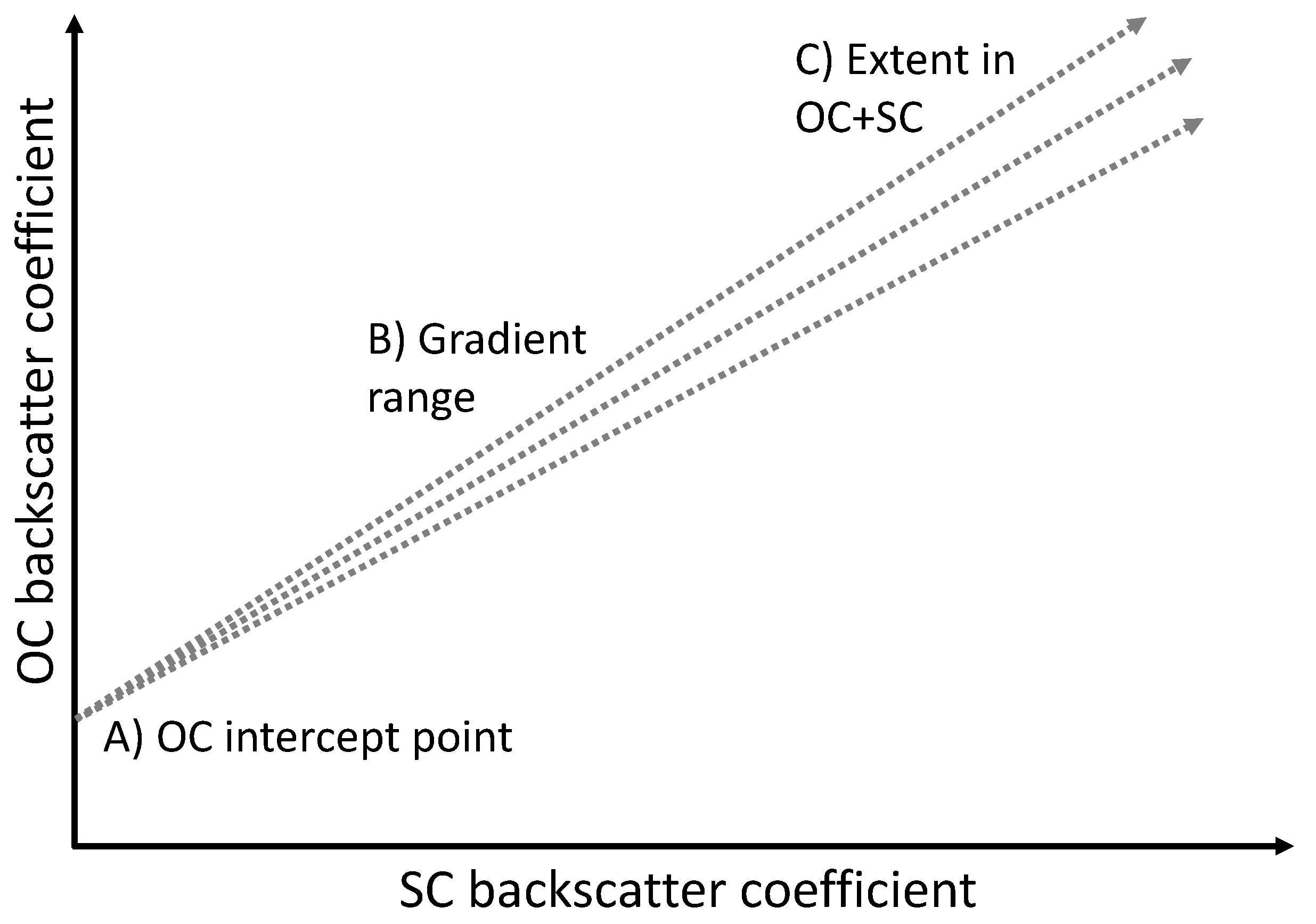
Radar polarimetry has traditionally focused on interpreting the CPR; high CPR values arise from significant surface roughness, such as impact ejecta (e.g., [67,68,69,70]), or due to the coherent backscattering effect in icy media (e.g., [17]). Virkki et al. [71] demonstrated that both the SC and OC enhancements can vary due to the abundance, size–frequency distribution, dielectric properties, and shape of wavelength-scale particles, so that CPR alone can hide part of the information that is visible in the full SC–OC backscatter coefficient space. Figure 5 summarizes visually the interpretation parameters: The (area-normalized) OC backscatter coefficient intercept point (A) describes the reflectivity of the surface without wavelength-scale scatterers, which can be used for deriving the effective electric permittivity of the surface composed of fine-scale regolith. Wavelength-scale scatterers on the surface or in the near-subsurface increase both the SC and OC backscatter coefficients, so that the gradient (B) depends on the shape, size–frequency distribution, and the dielectric properties of the particles with respect to the fine-grained regolith, and the extent (C) is directly proportional to the wavelength-scale particles’ abundance [71]. The method can be used for radar data at similar incidence angles, or if incidence angles between data sets differ significantly, after using a radar scattering law for normalization. An incidence angle difference between the sets can affect both the intercept point and the gradient, because the backscatter coefficient decreases as a function of the incidence angle and the observed backscatter coefficient is a combination of the quasi-specular and diffuse scattering. Also, the physical properties of the particles can affect both the gradient (B) and the extent (C), because the extent is a multiple of individual particles’ backscatter coefficients, which can have individually different SC and OC components [71]. The coherent backscattering effect would also further affect the gradient and the extent by likely lowering the gradient and increasing the extent, but its impact has not yet been well quantified. Rivera-Valentin et al. [31] applied the method to Arecibo radar observations of Mercury.
3.6.2. Full/Quad-Polarization Radars
As described in the previous section, conventional Earth-based planetary radar instruments transmit circular polarization, and receive both senses of circular polarization, resulting in SC and OC image pairs. In observations where the complex cross correlation between the two received channels (or, the relative phase of the two signals) is also measured, the full polarization state of received signals can be obtained. This is achieved by measuring the Stokes vector, from which classical child parameters such as the degree of depolarization and the degree of linear polarization may also be determined [74]. The architecture of this dual-circular polarimetric mode, along with the hybrid dual-polarimetric mode implemented in the Mini-RF radars (Mini-SAR on Chandrayaan-1 and Mini-RF on LRO) are forms of compact polarimetry [75], which is a subset of the fully polarized SAR configuration. However, the gold standard among polarimetric radars is the fully polarized case, in which the intrinsic data product is the 4 × 4 scattering matrix of each resolved element in the scene [74]. After applying certain symmetry relations, this may be reduced to a 3 × 3 array, such as a compressed Stokes matrix or the compressed scattering matrix [76]. These reduced forms are known commonly as fully polarimetric or quadrature-polarimetric SAR (quad-pol). The DFSAR instrument aboard Chandrayaan-2 is the first fully polarimetric SAR outside an Earth orbit. The architecture of this radar instrument supports multiple polarimetric modes of operation [77] and illustrates the value of quad-polarimetry for lunar and planetary applications [39]. DFSAR under the fully polarimetric mode alternately transmits two orthogonal linear polarizations and records both received linear polarizations (HH, HV, VH, and VV). This architecture allows more information to be extracted compared to single- and dual-pol SAR data (e.g., [39,78]). Polarimetric channels acquired in quad-pol mode maintain their relative phase, so they can be combined coherently to form new channels [76] or to compute statistical higher-order parameters by target decompositions (e.g., [79]). Moreover, quad-pol data produce a unique scattering matrix using any combination of transmitted and received orthogonal polarizations (e.g., linear, elliptical, hybrid), which permit analysis of the surface scattering behavior in all possible configurations of the transmitted and received signal polarizations.
In the monostatic backscatter alignment quad-pol mode operation, DFSAR transmits two orthogonal polarizations on a pulse-to-pulse basis and receives the scattered waves in two orthogonal polarizations (in the same basis as used for transmission). By this procedure, the radar acquires polarimetric scattering information as a 2 × 2 complex matrix called the Sinclair scattering matrix [80]. This scattering matrix relates the two-dimensional transmitted (subscript ) and received (subscript ) electric field vectors [76,81]:
where all the elements are complex valued, and the subscripts H and V indicate horizontal and vertical polarization, respectively. The factor , where is the wavenumber, takes into account the propagation effects both in amplitude and phase and expresses the attenuation for a spherical wave of a radius that equals the distance (r) between the scatterer and the radar. In this expression, the diagonal elements of the scattering matrix are termed “co-polar”, since they relate the same polarization for the incident and the scattered fields. The off-diagonal elements are known as “cross-polar” terms as they relate orthogonal polarization states. In monostatic configurations like that of DFSAR, becomes symmetric, i.e., S = S for all reciprocal scattering media (e.g., [76]).
In a sense, a quad-pol SAR receives the time-averaged samples of scattering from a set of different single targets, which is referred to as a “distributed radar target”. Such distributed targets (natural surfaces) can be analyzed more precisely by introducing the concept of space- and time-varying stochastic processes, where the target or the environment can be described by the second-order moments of the fluctuations, which will be extracted from the polarimetric coherency or covariance matrices [76]. If the scattering matrix is averaged in a covariance or coherency matrix for incoherent scattering, the number of independent parameters becomes nine, compared to one and three parameters by single polarization or dual-polarization SAR systems, respectively. Similar to the decomposition techniques applied to compact-pol SAR data (e.g., m- decomposition method; see the next section), scattering decompositions are widely applied over quad-pol SAR data for interpretation, physical information extraction, segmentation, and/or as a pre-processing step for geophysical parameter inversion (e.g., [76,79,82]). In general, the decompositions from the coherency or covariance matrices obtained from quad-pol SAR data can be grouped into two classes: eigenvector- and eigenvalue-based decompositions and model-based decompositions [79]. Moreover, to determine the CPR from quad-pol SAR measurements, it is straightforward to calculate the backscatter coefficients () in the two circularly polarized components from the linearly polarized terms as given below [83,84]:
where Re denotes the real part of the co-polarized correlation. Note that the above equations are derived by assuming that there is no correlation between the cross-polarized (HV, VH) and like-polarized (HH, VV) linear components for natural surfaces (e.g., [69]).
3.6.3. Decomposition
In the 2010s, more elaborate radar polarimetry methods and interpretations were introduced in the planetary radar community as an expansion from terrestrial radar imaging analysis. Raney et al. [85] developed the decomposition method to visualize the spatial distribution of different scattering processes in radar images of the Moon using observations from LRO’s Mini-RF. In the name of the method, m refers to the degree of polarization and to the degree of ellipticity and the sign of rotation of the polarization ellipse. Such decomposition products are RGB images, where the color intensity follows the power measured from the double-bounce (red), depolarized (green), and odd-bounce (blue) scattering components, as proposed by Raney et al. However, the interpretation of the number of bounces was questioned by Hickson et al. [86] in their work using the same method for asteroids. They argue that second-order scattering by a pair of wavelength-scale particles does not typically have as strong a depolarization effect on backscattering. Single scattering by a rounded particle, though, with a very rough surface and a size parameter (, where a is the effective radius) of about 3 can have a strong depolarizing effect at bistatic (phase) angles greater than 30 [86]. Further, including the third dimension in a dihedral model could change the observed polarization as well.
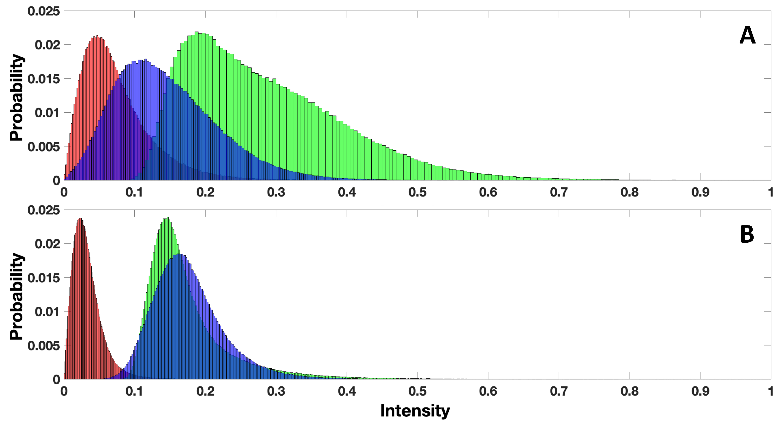
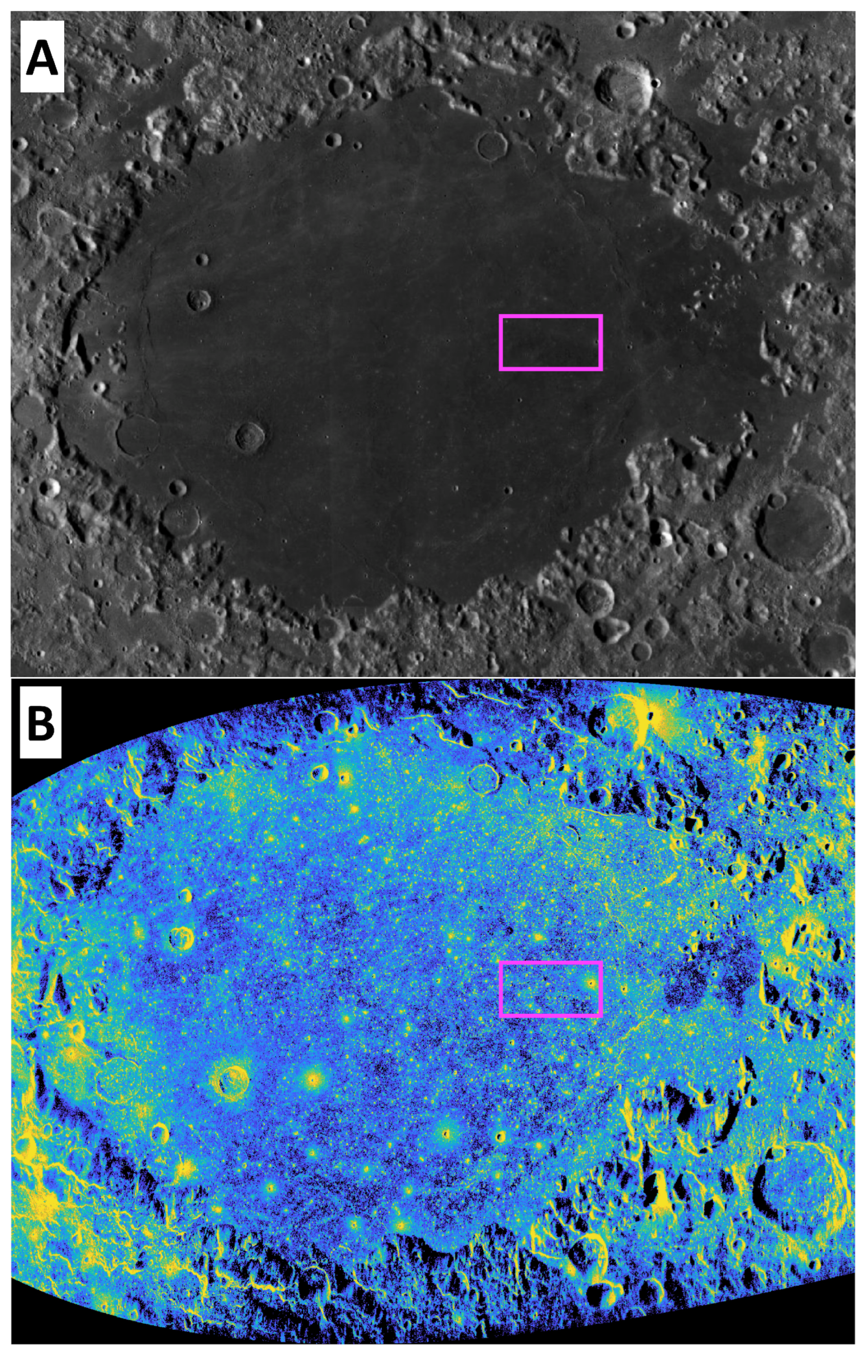
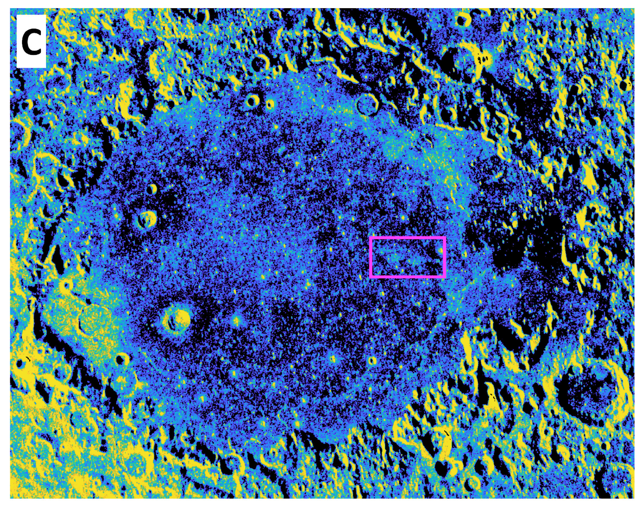
In Figure 6, we show an example decomposition map product focusing on Gardner crater (33.8N, 17.7E, diameter = 17.6 km) using Mini-RF S-band monostatic observations. Within the wall of Gardner crater, the scattering decomposition highlights landslide features on its walls. The landslides appear as yellow, which is due to a combination of depolarizing wavelength-scale scatterers and wall roughness, as well as the scattering geometry. On the other hand, the crater floor and most of the nearby areas are dominated by blue, which, due to attenuation, is likely dominated by power from single, quasi-specular reflections by areas with no wavelength-scale scatterers. To illustrate this difference, in Figure 7 we show the histogram of RGB intensity from the crater wall and nearby terrain. As can be seen, from the crater wall the distribution of depolarized/volumetric backscatter is skewed with a long tail as compared to the distribution of depolarized backscatter from the background terrain. This suggests an overabundance of fine-scale regolith. Furthermore, the distribution of red is broadened at the crater wall as compared to the background terrain, which is well explained by an overabundance of centimeter- to decimeter-scale rocky material. Additionally, the distribution of blue is shifted at the wall to lower values, which is well explained by the geometric complexity of wall material and a lack of radar-facing, smooth facets.
4. Radar Observations of the Moon
4.1. Ground-Based Observations
The first detection of radar signals reflecting from the Moon occurred in 1946. The so-called “Project Diana” was conducted by the US Army Signal Corps, and this achievement is considered the start of planetary radar astronomy. Since then, the Moon has been observed over a broad range of radar wavelengths, from 2.2 cm to 7.5 m, from ground-based telescopes such as the Arecibo Observatory, Goldstone Solar System Radar, MIT Haystack Observatory, Jicamarca Radio Observatory, and most recently the Green Bank Observatory. Early observations of the Moon set the stage for our current understanding of radar scattering processes under planetary relevant conditions. Such measurements led to the formulation of the often used Hagfors [61] and Muhleman [87] scattering models, which describe the expected backscatter from an undulating surface as a function of incidence angle, dielectric permittivity, and the root mean square of surface heights (i.e., roughness). Such semi-empirical models are still used across planetary radar astronomy to help infer regolith properties.
The observatory that has primarily been used for lunar radar science over the years has been the Arecibo telescope, which has provided dual-polarization observations of most of the near-side of the Moon at the P- (70 cm, 430 MHz) and S-band (12.6 cm, 2380 MHz). Due to the time it takes to switch between transmission and receiving modes, these observations were produced using a bistatic configuration, where Arecibo would transmit and the Robert W. Byrd Green Bank Telescope in West Virginia would receive [88,89]. Because the beam size of the Arecibo telescope is significantly smaller than the Moon, multiple observing sessions were needed; however, this also meant that the north–south ambiguity could be avoided by pointing the telescope at one hemisphere. In addition, because of the moon’s complicated and very slow apparent rotation as viewed from a point on Earth, the Doppler equator shifts over time, so that different points on the surface are affected by the north–south ambiguity, allowing most of the surface to be imaged. Similarly, the Moon’s libration allows imaging of approximately 200 of longitude by choosing whichever spot is most observable at any given observing session. Because of the very slow rotation, the Doppler resolution must be extremely fine to produce useful planetocentric projected spatial resolution. For the 70 cm observation, single radar looks were over 900 s, so that only a few observations could be made in the ∼2.5 h daily Arecibo observing window.
The two different observing wavelengths with Arecibo, 12.6 and 70 cm, allowed observations at different penetration depths. The 70 cm observations are particularly apt for identifying lava flows that are partly buried by regolith, while 12.6 cm observations are good for studying regolith properties. For example, in Figure 8, we show Arecibo S- and P-band SC backscatter radar maps of Mare Crisium (17N, 59E) [88,89], along with an image from the LRO’s wide angle camera for context. The S-band SC backscatter map highlights recent impact craters within the basin and their ejecta deposits more clearly than the P-band map. On the other hand, an ancient lava flow is markedly noticeable in the P-band image and not in S-band. This implies that the feature is likely buried at or below the S-band penetration depth (∼1 m) and/or is dominated by structure on the order of decimeters to meters rather than centimeters to decimeters. Indeed, multi-wavelength radar studies of the Moon have helped to reveal its volcanic history and provided important stratigraphic information (e.g., [90,91]). In particular, Arecibo P-band observations have helped to complete the inventory of lunar mare basalts by revealing buried features, such as cryptomaria [92], which are only otherwise visible by surface exposure through impact cratering. Longer wavelengths, such as the 6 m Jicamarca observations, can provide further constraints on ancient activity (e.g., [2]).
Figure 8 also demonstrates the impact of metal abundance in the lunar regolith. As demonstrated by [93], increased TiO abundance is related to decreased radar backscatter on the Moon due to the increased loss tangent. Indeed, the particularly radar-dark region in both the S- and P-band images in Figure 8 located at the center right of the image is associated with measured TiO of >7%, as compared to the bulk of Mare Crisium which is <4% [94]. Thus radar scattering on the Moon is associated with regolith’s physical properties (e.g., size frequency distribution of scatterers and their shape, topographic roughness) as well as composition due to the variation in TiO. This is related to the mineral ilmenite, which is associated with mare basalts. Another compositionally dependent radar signature that has been searched for on the Moon is that of water ice. Lunar permanently shadowed regions (PSRs), much like those on Mercury, have thermal environments that would allow for water ice accumulation [95,96]. However, unlike for Mercury, Arecibo S-band radar observations of the lunar poles did not reveal anomalously high radar backscatter or CPR [97]. This may suggest that (1) the lunar poles do not contain buried water ice; (2) they do but it is buried below the P-band radar penetration depth; and/or (3) the water ice is not in a coherent, nearly pure slab, but rather pore-filling or well-mixed with the regolith.
4.2. Lunar Orbital Radars
India’s lunar Chandrayaan-1 was the first SAR to orbit and observe the Moon. Launched in October 2008, Chandrayaan-1 was shortly followed by NASA’s Miniature Radio-Frequency (Mini-RF) instrument aboard the Lunar Reconnaissance Orbiter, which launched in June 2009. Chandrayaan-1 operated at 12.6 cm, while Mini-RF operates at both 4.2 and 12.6 cm. They operated together until communications were lost from Chandrayaan-1 in August 2009. The first radar experiment on the Moon, though, was conducted with the Clementine spacecraft in 1994 [98]. Clementine conducted a bistatic radar experiment by transmitting an S-band signal through its high-gain antenna, which reflected off the south pole of the Moon and was received by the DSN. The advantages of orbital radar assets over ground-based planetary radar observations of the Moon are improved spatial resolution, varying viewing geometries over regions during repeat passes, and fully polarimetric data sets. An additional advantage is that an orbital platform allows for radar imaging of the lunar far side.
The search for water ice at the lunar poles has continued with orbital radar assets. The 13.2 cm bistatic radar experiment aboard the Clementine spacecraft identified a localized coherent backscatter opposition affect associated with some PSRs at the lunar south pole, but not its north pole [98]. These results, though, were not shown to be unique and anomalous for the region in later studies [99]. Continued experiments with dedicated SARs have been similarly unsuccessful. Using monostatic Mini-RF and Chandrayaan-1 observations, Neish et al. [100] studied the S-band CPR of Cabeus crater, the site of the Lunar Crater Observation and Sensing Satellite (LCROSS). This spacecraft conducted an impact experiment on the Moon in an attempt to reveal buried volatiles. Although the LCROSS experiment identified water-related signatures in the resulting ejecta plume [101], pre- and post-impact Mini-RF S-band radar images of the region did not present anomalous backscatter [100]. Analysis of the initial CPR maps from the Mini-SAR on Chandrayaan-1 suggested that some polar craters showed high-CPR deposits only in their interiors and have low CPR values in adjacent deposits beyond their rims [102]. This finding was also supported by Mini-RF data by [103] who identified these features as “anomalous” craters. The interiors of these initially identified anomalous craters are wholly or in large part in permanent shadow and correlate with proposed locations of polar ice, as suggested by Lunar Prospector neutron spectrometer data [104]. As such, Refs. [102,103] proposed that these relations are consistent with deposits of water ice. However, such anomalous-CPR craters were also later identified outside of the polar regions [105,106], and were shown to also be well explained by the existence of blocky rock populations [107], and the size–frequency distribution and/or shape of the scatterers [71] within the crater. Later, in a bistatic radar experiment with Mini-RF as a receiver and Arecibo as a transmitter, an opposition effect was observed associated with Cabeus crater [108]. The response was suggested to significantly differ from that of crater ejecta and background terrain and to be potentially indicative of near-surface water ice.
A plethora of measurements at non-radar wavelengths support the existence of surface water ice at the lunar PSRs (e.g., [101,109,110,111,112,113,114]). Nevertheless, to date, radar investigations have not provided unique identification of buried water ice. This stark contrast to observations of Mercury’s poles (see next section) provides constraints on the delivery of water ice to the Moon relative to Mercury. Impact-induced regolith mixing models suggest that water ice deposits will be reworked into the background over scales of hundreds of millions of years for both bodies [115]. As such, the difficulty in radar detection of ice at the Moon may suggest intimate mixing with the regolith and burial at great depths, while on Mercury the clear detection of water ice may suggest a recent voluminous delivery of water ice. Continued dual-frequency orbital radar missions, such as the Indian Space Research Organization’s (ISRO) DFSAR aboard Chandrayaan-2, though, may provide new insights into the nature of lunar ice. DFSAR is the first to observe the Moon at L-band in addition to S-band. A comparison of the different depths probed by these wavelengths, along with the fully polarimetric data set and improved radar scattering models, may help to identify the nuanced radar signature from an intimate mixture of ice and regolith.
Orbital radar data has also proven to be an extremely useful tool for studying the geology of the lunar surface. With a now global view of the Moon, we can confirm the ground-based measurements that suggest the radar scattering properties of the Moon are broadly related to the mare–highlands dichotomy. The highlands have higher radar backscatter, likely due to a lower loss tangent in the regolith, which allows for more scattering from subsurface rocks [38]. Orbital radars also gave us our first look at the scattering properties of the global crater population of the Moon. These observations confirmed earlier ground-based data that suggested that impact melt deposits were among the rough materials on the Moon [89]. This unique property allowed for the construction of the first global data set of lunar impact melts since the 1970s [116]. It has also revealed melt deposits in unusual locations, such as the Tycho antipode [117]. Moreover, the fully polarimetric DFSAR data were utilized to estimate the dielectric constant [118] as well as surface roughness [119] at selected regions, and to provide new information on volcanic features such as pyroclastic deposits [120] and irregular mare patches [121].
5. Radar Observations of the Planets
5.1. Mercury
Radar observations of Mercury provided the first compelling evidence of volatiles within PSRs of polar craters. Full-disk radar mapping of Mercury conducted via monostatic Arecibo S-band (12.6 cm, 2380 MHz) radar observations [14] and bistatic observations, where the Goldstone 70 m antenna transmitted in X-band (3.5 cm, 8560 MHz) and 26 antennas of the Very Large Array received backscattered echoes [13], identified anomalously bright features at both poles. The features were associated with CPR > 1. Together these radar properties were reminiscent of the scattering behavior of the icy moons of Jupiter [8,122,123] and the Martian south polar layered deposits [124]. In subsequent Arecibo radar observations, delay and Doppler planetocentric projected spatial resolutions were improved to as fine as 1.5 km [125,126], allowing for tracking of the anomalously high reflectivity to crater-sized features.
In Figure 9, we show an example delay–Doppler image of Mercury’s north polar radar-bright features using the observations presented in [31], which were processed to a delay resolution of 1.5 km. For these features, thermal models demonstrated that within some 10 of the poles most crater geometries would result in PSRs with temperatures low enough to permit stable water ice at the surface, and to lower latitudes if insulated by a thin layer [127,128]. Thus, the properties of the radar-bright features at Mercury’s poles have been interpreted as resulting from scattering from water ice, with their high reflectivity likely due to the coherent backscatter effect [15,17].
The ground-based-radar-enabled discovery of ice at Mercury’s poles served as one of the motivators for NASA’s MESSENGER mission to Mercury, which launched in 2004, began science operations at Mercury in 2011, and concluded in 2015. Detailed observations by the MESSENGER spacecraft confirmed that radar-bright features are associated with PSR locations [129,130] and provided further support for the water ice interpretation as it found that the north polar region was on average enriched in hydrogen [131]. At the same time, though, MESSENGER observations revealed new complexities. First, not all Mercurian PSRs are associated with a radar-bright feature [130,132]. This may provide constraints on the source and timing of volatile delivery and deposition. Alternatively, the water ice content within some PSRs may be too thin or buried too deeply to be detected by S-band radar observations. Furthermore, MESSENGER observations surprisingly found that many of the locations of radar-bright features were optically darker than the surrounding terrain [133]. This would suggest that ice is not surficially exposed at these locations, but rather buried beneath a thin low-reflectance, perhaps organic-rich, material [134].
The heterogeneity of the Mercurian putative ice deposits revealed by MESSENGER motivated a renewed radar investigation. Leveraging the high-resolution topography data from MESSENGER, refs. [31,135] paired new Arecibo S-band radar observations with a topography-corrected radar incidence angle map to investigate the scattering properties of the features. In their work, they showed that some northern radar-bright features are associated with a distinct pattern in their properties, whereby a central high reflectivity and high-CPR region is surrounded by lower backscatter in a gradational pattern. Radar scattering modeling suggests that high reflectivity regions within PSRs are well characterized by nearly pure water ice decreasing out to >20% impurities by volume [31]. Thus, the purest ice deposits at Mercury are likely surrounded by water-ice-rich regolith. This could be due to lateral mixing induced by impact gardening and/or the local thermal environment. Further work comparing the radar backscatter with detailed thermal modeling of the largest northernmost craters, Kandinsky, Tolkien, Chesterton, and Tryggvadóttir, found that overall radar brightness is correlated well with temperature variations [136]. Their work also identified regions where surface ice is thermally stable but the radar backscatter is much lower than the brightest regions. As such, additional local-scale heterogeneities exist within the northernmost Mercurian PSRs.
Beyond investigations of volatile deposits within PSRs, radar observations of the mid-latitudes have also revealed geologic diversity that is similarly beneficial to comparative planetology. Of particular note are impact crater rays [137,138], which are optically bright, narrow, filament-like features that extend radially from some fresh impact craters across the Solar System. Although their optical brightness is typically due to either exposure of fresh, unweathered material and/or compositional-related albedo differences in exposed material compared to the background terrain (e.g., [139]), rays are bright at radar wavelengths due to an enhancement in wavelength-scale complexity along the ray’s path. Comparisons between rayed craters on the Moon and Mercury using radar observations along with other wavelengths helps to reveal the processes that led to their formation as well as subsequent evolution [138]. Indeed, radar observations strongly suggest that rays are primarily formed through secondary cratering. This is of particular importance for planning sample return missions in order to understand the provenance of regolith samples (e.g., [140]).
5.2. Venus
Venus’ thick atmosphere, which is opaque at visible wavelengths, has made radar the primary means of studying its surface. These observations go back many decades, to the first accurate determination of the rotation rate of Venus in the 1960s [4]. In the 1970s and 1980s, ground-based and orbital platforms returned global topography data and low-resolution (km scale) regional radar images of Venus (e.g., [141,142]). The most comprehensive imaging of Venus was completed by the Magellan spacecraft in the early 1990s. This returned high-resolution (∼100 m) radar images of 98% of the surface of Venus [143].
One of the most intriguing discoveries made by Magellan was the occurrence of a sharp shift to high-reflectivity, low-emissivity material at a specific altitude on Venusian mountains [144]. The exact nature of this material remains unknown, but may be consistent with a ferroelectric mineral such as a perovskite [145]. Magellan images also revealed a wide range of volcanic features, including familiar features like shield volcanoes and lava flows, but also unusual structures such as flat-topped pancake domes and ring-shaped coronae [146]. A key question in Venusian science is whether or not the planet is volcanically active. Ground-based imaging of Venus between 1988 and 2012 did not reveal any obvious changes in radar properties consistent with volcanism [147]. However, a recent analysis of Magellan data from February and October 1991 revealed a volcanic vent that changed shape and the possible presence of a new lava flow in the eight months between observations [148].
Additional ground-based observations of Venus continued up until 2020, just prior to the collapse of the Arecibo telescope [30]. The observations have provided polarimetric radar data of Venus (SC and OC) not available from Magellan, but at much coarser resolution (several km vs. 100 m). The polarimetric data have revealed that most Venusian lava flows have CPR values less than 0.3, consistent with smooth pahoehoe surfaces [149]. A number of fine-grained mantling deposits were also identified around impact craters and lava flows on Venus, characterized by low CPR and a high degree of linear polarization [150]. No additional radar images of Venus can be acquired with current ground-based assets, but several orbital missions carrying SAR instruments with interferometric and dual-polarimetric capabilities are planned in the coming years (see Section 7).
5.3. Mars
Radar images of Mars are limited to a few low-resolution, ground-based observations completed at X-band (3.5 cm) and S-band (12.6 cm). The first radar images of Mars were conducted in 1988 using Goldstone and the Very Large Array (VLA) in a bistatic configuration [124]. These low-resolution (170 km) X-band images revealed radar-bright features near Mars’s equatorial volcanoes, a radar-dark feature (dubbed “Stealth”) correlated with a low-density, rock-poor deposit, and a radar-bright feature associated with the south polar ice cap. Radar image processing improved during the 1990s and 2000s, utilizing a novel “long-code” method for delay–Doppler imaging [151]. This technique addressed issues associated with overspreading in the radar echoes due to Mars’s rapid rotation, and produced the first images of Mars at S-band [152]. Data acquired by Arecibo during the 2005–2012 opposition of Mars produced the highest-resolution radar images (∼3 km) of Mars to date [29,153]. These images have revealed features unseen in optical images of Mars. One of the more surprising discoveries is the presence of many lava flows with CPRs that exceed unity. This property is unusual for terrestrial lava flows, and suggests that Martian lava flows have blocky or disrupted surfaces [154]. These data also provided detailed radar images of the Martian polar ice caps. Their radar polarization properties are consistent with the coherent backscatter effect associated with relatively pure ice [153]. With the collapse of the Arecibo Observatory in 2020, it is no longer possible to obtain radar images of Mars. New ground-based or orbital observatories—such as the proposed International Mars Ice Mapper (I-MIM) mission—are needed to produce new, higher-resolution radar images of Mars.
Radars have also been used to probe the subsurface of Mars. Three radar sounders have reached Mars and are still in operation today, namely, MARSIS, aboard ESA’s Mars Express spacecraft [51], SHARAD, on NASA’s Mars Reconnaissance Orbiter [34], and MOSIR, on Tianwen-1 [53]. As ice is one of the most transparent natural materials at the frequencies employed by radar sounders, the Martian polar caps have been prime targets for observation. Their thickness and volume were thus measured, allowing an estimate of their total water ice content [35], and their interior layering was mapped to study their origin and evolution shaped by Martian climate cycles [32]. Although covered by layers of rocky debris, ice was found also at mid-latitudes [155], and is thus potentially accessible by future human explorers, while the enigmatic Medusae Fossae Formation has been found to be radar-transparent, but no conclusive evidence of the presence of ice in its interior could be provided [156]. Radar sounding also discovered layers of CO ice in the polar caps [157], while evidence for the presence of ground water ice has been found in the northern plains of Mars [158].
More recently, bright echoes at the base of the southern polar cap have been interpreted as being caused by the presence of liquid water [33,159]. Because of the very low temperatures expected in that area, it was proposed that the waters are hypersaline perchlorate brines, known to form at Martian polar regions and thought to survive for an extended period of time on a geological scale. Because of its significance in the study of the biologic potential of Mars, the identification of liquid water has been closely scrutinized by the scientific community at large, and several counterarguments and alternative interpretations of the MARSIS measurements have been proposed over the last four years. Although the debate has yet to reach a conclusion, geologic evidence, all experimental work, and most electromagnetic modeling favor the presence of brines, possibly as interstitial fluid in sediments [160,161,162,163,164,165,166,167]. Dense measurement coverage in the polar regions has enabled 3-dimensional processing of the sounding data to improve resolution and better map continuous structures in the ice caps [168,169].
5.4. The Galilean Moons
The Galilean moons are among the most interesting planetary objects in terms of their radar-scattering properties. They were first observed in 1976 at Arecibo [8,170]. Due to the high abundance of ice on Europa, Ganymede, and Callisto, the radar albedo and the SC radar cross-sections are anomalous compared to other planetary objects. Hapke [17] used laboratory experiments to show that the enhancements in both the reflectivity and the polarization are caused by the coherent backscattering effect. This theory has been supported via various numerical models [171,172].
Two spacecraft missions to Europa equipped with radar sounding systems are planned in the near future: ESA’s Radar for Icy Moons Explorer (RIME) instrument onboard Jupiter Icy Moons Explorer (JUICE) [173,174], and NASA’s Radar for Europa Assessment and Sounding: Ocean to Near-Surface (REASON) onboard Europa Clipper [175,176]. These missions have a pioneering opportunity to characterize the subsurface of Europa using radar sounding and the processes that shape Europa’s unique icy surface.
5.5. The Moons and Rings of Saturn
The Saturnian system is the most distant radar-detected planetary object in the solar system. Radar observations by ground- and space-based assets have returned important information about its rings and moons. The first radar observations of Saturn’s rings occurred in the early 1970s [177]. These observations demonstrated that the ring particles are at least cm sized or greater; these sizes were required in order to have an observable radar echo at S-band (12.6 cm). In the subsequent decades, numerous other ground-based radar measurements were acquired of the rings (e.g., [178,179]), revealing more detailed information about their geometry.
Ground-based radar observatories have also made several observations of Saturn’s moons, including Titan [180], Iapetus [181], Rhea, Dione, Tethys, and Enceladus [182]. The circular polarization ratios of the Saturnian moons are somewhat lower than those of the Galilean satellites (Table 1), but still consistent with abundant subsurface volume scattering due to the presence of water ice. The observed differences between the Galilean and Saturnian moons are likely due to differences in the composition of their near subsurfaces. A likely candidate is ammonia, as its presence in the Saturnian system could increase the microwave absorption of water ice. In addition, ground-based radar observations of Titan revealed a number of specular reflections from its surface. These observations suggested the existence of large areas that are relatively smooth at the cm scale [183], likely due to the presence of paleolakes or paleoseas [184].
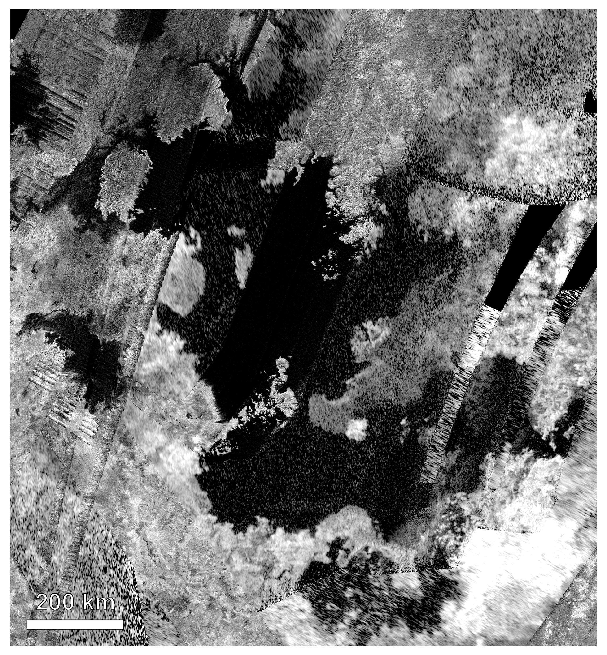
In 2004, a space-based asset began to collect information about the Saturn system at radar wavelengths: the Cassini RADAR instrument [185]. Cassini RADAR made a number of observations of Saturn’s mid-sized moons in the Ku-band (2.2 cm). These observations revealed a trend of decreasing radar albedos as one moves outward in the Saturnian system [186]. As discussed above, this is likely due to increasing water ice contamination by ammonia [187]. However, the Cassini RADAR was primarily used to map the surface of Titan for the first time at high resolution [188]. Radar observations through its hazy atmosphere revealed the presence of a surprisingly Earth-like world, dominated by exogenic processes such as aeolion and fluvial modification [189,190]. The latter process is the result of an active “hydrological” system on Titan, with methane as the working fluid. Cassini also made the remarkable discovery that Titan has large bodies of liquid near its poles [36], making it the only place in the solar system other than Earth to have surface liquids (Figure 10). Soundings by the Cassini RADAR produced echoes from the bottoms of these lakes, and the derived loss tangent is consistent with a methane-rich composition [191].

Table 1.
Radar properties of the terrestrial planets, the Moon, and the radar-observed moons of Jupiter and Saturn.
Table 1.
Radar properties of the terrestrial planets, the Moon, and the radar-observed moons of Jupiter and Saturn.
| Object | OC Radar Albedo | SC Radar Albedo | CPR | Wavelength | References |
|---|---|---|---|---|---|
| Mercury | 0.06 | 0.005 | 0.1 | 12.6 cm | [44,192] |
| Venus | 0.11 | 0.01 | 0.1 | 12.6 cm | [44] |
| Moon | 0.07 | 0.007 | 0.1 | 12.6 cm | [44] |
| Mars | 0.08 | 0.02 | 0.3 | 12.6 cm | [44] |
| Europa | 12.6 cm | [193] | |||
| Europa | 3.5 cm | [193] | |||
| Ganymede | 12.6 cm | [193] | |||
| Ganymede | 3.5 cm | [193] | |||
| Callisto | 12.6 cm | [193] | |||
| Callisto | 3.5 cm | [193] | |||
| Enceladus | 12.6 cm | [182] | |||
| Tethys | 12.6 cm | [182] | |||
| Dione | 12.6 cm | [182] | |||
| Rhea | 12.6 cm | [182] | |||
| Titan * | 12.6 cm | [183] | |||
| Iapetus (L *) | 12.6 cm | [181] | |||
| Iapetus (T *) | 12.6 cm | [181] |
* For Titan, the values have been estimated visually from Figure 2 in [183]. For Iapetus, “L” isfor the optically dark leading hemisphere and “T” is for the optically bright trailing hemisphere.
5.6. The Radar Scattering Properties of Planets and Moons
In the subsections above, we have described the radar properties of the planets and moons in our solar system. In the table below (Table 1), we summarize the radar albedos and CPR values for these objects. The table is divided in three sections: the inner solar system objects, the Galilean moons, and the moons of Saturn, and highlights the differences and similarities in the radar scattering properties between the groups as well as inside each group. The global radar-scattering properties of the inner solar system objects are overall modest compared to many of the moons of Jupiter and Saturn, which can be likely attributed primarily to the global characteristics (abundance, spatial distribution, and purity) of ice on each object.
6. Radar Observations of Small Solar System Objects
6.1. Asteroids
Due to the rapid fall-off in radar power with distance, the majority of radar-observed SSSOs have been NEAs. Only 138 main-belt asteroids (MBAs) have been observed using radar compared to more than a thousand NEAs (https://echo.jpl.nasa.gov/asteroids/PDS.asteroid.radar.history.html, accessed on 26 November 2023). The reason can be seen in Equation (1): because the received power falls inversely proportional to the fourth power of distance, the targets nearby are more easily observable. The first radar-observed NEA was (1566) Icarus in June 1968, which was observed bistatically at Goldstone and Haystack. From this point up until the end of the 1970s, only up to one asteroid was observed per year. The number increased to 4–15 per year through the 1980s and 1990s, and continued to increase through the 2000s and 2010s as instruments were upgraded and NASA began to provide more funding for asteroid observations. The peak number of 123 NEAs were observed at Arecibo in 2019 [43], plus three more using the DSN telescopes at Goldstone and Canberra (https://echo.jpl.nasa.gov/asteroids/PDS.asteroid.radar.history.html, accessed on 26 November 2023). The total number of unique radar-observed NEAs is currently above 1060 and counting, the exact number depending to a small extent on which objects count as successful detections. Note that the target location has to be known with a precision better than the beam width of the radar system to be observable.
Multi-body systems, i.e., binary and ternary asteroids, are of particular interest in terms of asteroid formation and evolution. They are also common: The fraction of near-Earth asteroids larger than 300 m in diameter that are multiple systems is estimated to be about 15% [194]. Planetary radar is a powerful instrument in detecting asteroid moons, because the delay–Doppler imaging, and in some cases even just the Doppler echo power spectra, can reveal the asteroid moons more distinctly than optical lightcurves. This is because the satellites often have their spins tidally locked to their orbits [194], which concentrates the radar echo into a very narrow frequency interval, so that they appear bright. To date, 69 multi-body systems have been observed using radar, starting with (1866) Sisyphus in 1986 (though it was not recognized at the time). The first well-characterized near-Earth binary system, 2000 DP107, was discovered using radar in 2000 [195]. Some of the systems were confirmed as binary or ternary systems using radar, whereas some were suspected as binary systems already before the radar observations. In some cases, a satellite that is suspected based on optical observations is not detected using radar, which could be due to an unfavorable observation geometry, bad signal-to-noise ratio, or a misinterpretation of the lightcurve.
The first ternary system, (153591) 2001 SN263, was observed in 2008 at Arecibo [196], and three other ternary systems have been observed since, with the best delay–Doppler images obtained for (3122) Florence in 2017. The other two ternary systems are (136617) 1994 CC and (348400) 2005 JF21. Other multi-body systems of special interest are equal-mass binaries, of which only four have been observed. The best images of an equal-mass binary system were obtained for 2017 YE5 in 2018 (Figure 3). The other three equal-mass binary systems are (69230) Hermes, 1994 CJ1, and (190166) 2005 UP156 [197,198].
As mentioned in Section 3, delay–Doppler imaging is arguably the best ground-based technique for the imaging of planetary bodies in the inner Solar system. It is particularly powerful for revealing the diversity of shapes and sizes of near-Earth asteroids [43]. Although optical lightcurves can be used for a convex-hull estimation of asteroids, only radar delay–Doppler images are able to directly image concavities. Therefore, radar images are key to understanding asteroids’ shape distribution and evolution. Optical and near-infrared observations can also estimate the asteroids’ size based on the reflectivity and an estimated albedo at their respective wavelengths, but a fine imaging resolution is required for a direct observation. Radar observations can, thus, help to validate the size estimation methods utilized at other wavelengths.
In Section 3.6, we described how the polarization of the radar signal could be used for the characterization of planetary surfaces. The radar-polarimetric analysis can contribute to the characterization of the composition of asteroids, especially in terms of X-type asteroids in the Tholen spectral classification system [199]. These asteroids have similar, flat VNIR spectra but can be subgrouped as P, M, or E type based on their geometric albedo (respectively, low, medium, or high albedo). Radar polarimetry is particularly powerful at identifying E-type asteroids, for which the CPR is anomalously high compared to other taxonomic types [200], whereas a high radar albedo can reveal the metal-rich M-type asteroids [25]. The albedo estimate requires a size estimate based on imaging or polarimetric data.
A wealth of literature exists on the radar scattering properties of asteroids. Some of the largest and most significant compilations are those by Magri et al. [26,201,202] for (dominantly) main-belt asteroids, Benner et al. [200] for CPRs of NEAs observed until 2008, and Virkki et al. [43] for recent observations of NEAs at Arecibo.
6.2. Comets
Comets are challenging radar targets for two reasons: first, and most importantly, they rarely come close enough to Earth to be observable; and second, their porous surfaces are poor radar reflectors, which makes them more challenging objects to observe compared to most asteroids. Thus, only 21 comets have ever been successfully observed using radar (https://echo.jpl.nasa.gov/asteroids/index.html, accessed on 26 November 2023).
When comets are observed, radar observations can reveal the scattering properties of both the nucleus and the coma (e.g., [203]). As with asteroids, the size, shape, and spin rate of the nucleus can be determined if the object comes close enough, though that is rare. If the coma contains cm-scale or larger particles, then these can also be observed. In radar Doppler echo power spectra, the nucleus typically appears as a narrow peak within a wide, lower-power band of the coma. The Doppler bandwidth of the nucleus is determined by its rotation rate, where the Doppler bandwidth of coma particles is determined by their spread in outflow velocity from the nucleus, which is typically hundreds of m/s, compared to the cm/s or m/s rotational velocity of the nucleus. The intensity of the coma is directly related to the number and size distribution of cm-scale and larger particles and can change from day to day depending on the variations in the size–frequency distribution of the coma particles and the observation geometry. The CPR of the coma may be used for investigating the coma particles’ wavelength-scale size–frequency distribution if observations at two different radar wavelengths are available [204]. Because comets are quite variable in size and dust production, some comets show only a nucleus echo, some show only a coma echo, and some show both. Figure 11 shows an example of the Doppler echo power spectrum for 73P/Schwassmann-Wachmann 3 (fragment C), which fragmented in 2006 as a result of returning to the inner Solar System. Here, an asymmetric coma is clearly visible due to the large number of wavelength-scale particles, while a large fragment of the nucleus is visible as a peak in the middle.
The only comet that has been visited by a spacecraft equipped with a sounding radar instrument is 67P/Churyumov–Gerasimenko (hereafter 67P). The Comet Nucleus Sounding Experiment by Radiowave Transmission (CONSERT) onboard the Rosetta spacecraft conducted a bistatic radar sounding experiment by propagating long-wavelength (90 MHz, 3.3 m) signals between the spacecraft and the Philae lander so that the signal traveled partially through the nucleus of 67P [56]. The experiment took place in November 2014 immediately after the landing of Philae, which coincidentally bounced off from the planned landing location to an unknown location. The unintended bounce made the calibration difficult, because the experiment began during an occultation rather than a clear visibility between the spacecraft and the lander. Still, the experiment succeeded in the detection of signals that had passed through the nucleus. The obtained data constrained the electric permittivity of the nucleus to 1.27, which further constrained its bulk density and porosity, as well as its scattering signatures. These data revealed the nucleus to be homogeneous at the wavelength scale [56]. Further, Heggy et al. [205] concluded that the meter-scale surface textures were more likely formed by thermal contractions of the shallow subsurface than representative of the primordial building blocks of the comet, because no volume-scattering signatures were detected.
7. The Future of Planetary Radar
7.1. Ground-Based Observations
Since the collapse of the William E. Gordon telescope of the Arecibo Observatory, ground-based radar capabilities have been significantly impaired. No facility with comparable capabilities currently exists; ground-based radar capabilities are now limited to those of the DSN telescopes, primarily Goldstone. The limitations are set by antenna sizes, transmission power, and scheduling. The DSN has an ongoing effort to improve their capabilities, dominantly driven by the need for improved spacecraft communications as the number of spacecraft increases and spacecraft communications evolve [206]. The DSN Aperture Enhancement Project includes building new antennas at each DSN location and installing new uplink and downlink systems, which would allow more efficient communications with the spacecraft. In terms of radar observations, these upgrades would benefit primarily the space-based radar systems. However, the planned modernization of the radar control systems at Goldstone would benefit the ground-based planetary radar observations as well.
The future development of ground-based planetary radar systems is currently seen as crucial for efficient planetary defense [207]. According to the recent report [207], future radar facilities will most likely be telescope arrays, which can be developed incrementally and have a lower risk of a single-point failure than one large telescope. However, the technical ability to transmit and receive coherent radar signals from planetary bodies with large arrays has not yet been properly established, and requires technological development.
The Green Bank Observatory has recently made significant development toward adding a Ku-band (13.7 GHz, 2 cm) radar transmitter in the 100 m Robert W. Byrd telescope [42]. The system is planned as a bistatic radar with a different location, such as the Very Long Baseline Array (VLBA) or, in the future, the next-generation Very Large Array (ngVLA) receiving. The current experiments have been limited to a low power of 700 W, but as much as 500 kW has been proposed.
In addition, China has recently announced the development of the China Fuyan (“Compound Eye”) facility in Chongqing, to be used for NEA observations and spacecraft communications. The three-phase project is currently at its second phase: building an array of twenty-five 30-m radio telescopes (https://www.globaltimes.cn/page/202302/1285461.shtml, accessed on 23 October 2023). In the first phase, four radar antennas with 16-m apertures have been successfully used for obtaining radar images of lunar craters. In the third phase, the number of radar antennas is planned to be increased to over one hundred.
7.2. Planned Radar Instruments on Future Spacecraft Missions
Space-based radar instruments have a bright future, with radar systems planned for several planetary spacecraft. Four missions to Venus were recently announced to fly radar systems in the near future: (1) the Venus Orbiter Mission (unofficially named Shukrayaan) was announced by the Indian Space Research Organisation to launch in December 2024; (2) the Venus Volcano Imaging and Climate Explorer (VOICE) mission was announced by the China National Space Administration to launch in 2026 and arrive at Venus in 2027; (3) the Venus Emissivity, Radio Science, InSAR, Topography, and Spectroscopy (VERITAS) mission was preliminarily planned by NASA’s Jet Propulsion Laboratory (JPL) to launch in 2029; and (4) EnVision was announced by ESA to be launched in 2031. VOICE will carry an S-band polarimetric SAR and a microwave radiometric sounder (MRS), while the Venus Orbiter Mission will carry an S-band fully polarimetric SAR and a high-frequency (HF) radar sounder. The Venus Interferometric Synthetic Aperture Radar (VISAR) instrument onboard VERITAS is an X-band radar system designed to generate global topographic data sets with an accuracy of 250 m horizontal and 5 m vertical accuracy. It will also collect SAR images at 30 m resolution, and produce the first active surface deformation map of a planet other than Earth at a vertical accuracy of 1.5 cm. The Venus Synthetic Aperture Radar (VenSAR) is an S-band dual-pol radar onboard EnVision [208]. EnVision will also carry the Venus Subsurface Radar Sounder (SRS), a fixed dipole antenna operating in the frequency range of 9–30 MHz, designed to probe the deeper subsurface of Venus.
The Galilean moon Europa will also have two different spacecraft radar systems probing its subsurface oceans: (1) ESA’s Radar for Icy Moons Explorer (RIME) instrument onboard the Jupiter Icy Moons Explorer (JUICE) [173,174], which launched in April 2023 and will arrive in the Jupiter system in 2031, and (2) NASA’s Radar for Europa Assessment and Sounding: Ocean to Near-Surface (REASON) onboard Europa Clipper [175,176], planned to launch in October 2024 and to arrive in April 2030. RIME is a radar sounder using a frequency of 9 MHz and could penetrate as deep as 9 km into the ice, whereas REASON is a DFSAR that uses both a 9 MHz and a 60 MHz frequency sounder.
Furthermore, Juventas Radar (JuRa), onboard ESA’s Hera mission, is planned to visit the (65803) Didymos-Dimorphos system for post-impact characterization of the target asteroid of NASA’s Double Asteroid Redirection Test (DART). The DART spacecraft successfully impacted Dimorphos in September 2022 and changed its orbital period around Didymos. JuRa will operate in the frequency range of 50–70 MHz, have a spatial resolution of 10–15 m, and will be the first instrument to probe the inner layers of an asteroid. Hera is planned to launch in October 2024 and to arrive in December 2026 [209].
In conclusion, seven decades of planetary radar observations have truly demonstrated the unique capabilities that the technique offers, but also that there remain discoveries to be made. Furthermore, the planned radar instruments on various spacecraft and the current and new Earth-based planetary radar facilities in development will continue planetary radar science for decades to come.
Author Contributions
Conceptualization, A.K.V.; writing—original draft preparation, A.K.V., C.D.N., E.G.R.-V., S.S.B., D.C.H., M.C.N. and R.O.; writing—review and editing, A.K.V., C.D.N., E.G.R.-V., S.S.B., D.C.H., M.C.N. and R.O.; visualization, A.K.V., C.D.N. and E.G.R.-V.; supervision, A.K.V. All authors have read and agreed to the published version of the manuscript.
Funding
A.K.V. acknowledges support from Academy of Finland Grant No. 347627. E.G.R.-V. acknowledges support from NASA through the Solar System Observations (SSO) program under Grant No. 80NSSC19K0523 and the Lunar Reconnaissance Orbiter project under Contract No. NNN16AA05T. M.C.N. acknowledges support from NASA’s Near-Earth Object Observations and SSO programs through Grant Nos. NNX12AF24G, NNX13AF46G, and 80NSSC19K0523. Open access funding provided by University of Helsinki.
Data Availability Statement
All data displayed in this review article is of public domain; no new data were created. The Magellan data are available at https://pds-geosciences.wustl.edu/missions/magellan/index.htm. Images based on the Arecibo and Goldstone radar observations of asteroids (funded by NASA) are available at https://www.lpi.usra.edu/resources/asteroids/ and https://echo.jpl.nasa.gov/; the data are in the process to be made available at the NASA Planetary Data System Small Bodies Node. The Mini-RF data are available through https://pds-geosciences.wustl.edu/missions/lro/mrf.htm, Arecibo S-band data of the Moon are available at https://pds-geosciences.wustl.edu/missions/sband/index.htm, the Arecibo P-band data are available at https://pds-geosciences.wustl.edu/missions/lunar_radar/index.htm, and the data for the Cassini RADAR image of Kraken Mare are available at https://astrogeology.usgs.gov/search/map/Titan/Cassini/Global-Mosaic/Titan_SAR_HiSAR_MosaicThru_T104_Jan2015_clon180_128ppd. The mosaic of the optical image of Mare Crisium makes use of data from the Lunar Reconnaissance Orbiter’s Wide Angle Camera obtained from Applied Coherent Technology’s Quickmap at https://quickmap.lroc.asu.edu/layers?extent=37.1260837%2C5.8734242%2C77.2056205%2C28.6225597&id=lroc&showTerrain=true&queryOpts=N4XyA&layers=NrBsFYBoAZIRnpEBmZcAsjYIHYFcAbAyAbwF8BdC0yioA&proj=16&time=2023-12-01T13:37:02.794Z. The Arecibo S-band radar observations of Mercury were reported in [31] and of Comet 73P in [204].
Acknowledgments
Much of this work was performed at the Arecibo Observatory, which is a facility of the US National Science Foundation. The Arecibo radar program was a NASA project. Over the years, observatory operations have been led by Cornell University, SRI International, and the University of Central Florida. We thank the staff of the Arecibo Observatory for 60 years of dedicated service. Siempre estarán en nuestros corazones.
Conflicts of Interest
Author D.H. was employed by the MDA Geospatial Services Inc. and declares that the company had no role in the design of the study; in the collection, analyses, or interpretation of data; in the writing of the manuscript; or in the decision to publish the results. The remaining authors declare that the research was conducted in the absence of any commercial or financial relationships that could be construed as a potential conflict of interest.
Abbreviations
The following abbreviations are used in this manuscript:
| BPC | Binary phase coding |
| CONSERT | Comet Nucleus Sounding Experiment by Radiowave Transmission |
| CPR | Circular polarization ratio |
| DART | Double-Asteroid Redirection Test |
| DFSAR | Dual-frequency synthetic aperture radar |
| DSN | Deep space network |
| DSS | Deep space station |
| EISCAT | European Incoherent Scatter Scientific Association |
| ESA | European Space Administration |
| GPR | Ground penetrating radar |
| HF | High frequency |
| ISRO | Indian Space Research Organisation |
| JPL | Jet Propulsion Laboratory |
| JUICE | Jupiter Icy Moons Explorer |
| LCROSS | Lunar Crater Observation and Sensing Satellite |
| LPR | Lunar Penetrating Radar |
| LRO | Lunar Reconnaissance Orbiter |
| LRPR | Lunar Regolith Penetrating Radar |
| LRS | Lunar Radar Sounder |
| MARSIS | Mars Advanced Radar for Subsurface and Ionosphere Sounding |
| MBA | Main-belt asteroid |
| Mini-RF | Miniature Radio Frequency |
| NASA | National Aeronautics and Space Administration |
| NEA | Near-Earth asteroid |
| ngVLA | Next-generation Very Large Array |
| NSF | National Science Foundation |
| OC | Opposite circular |
| PSR | Permanently shadowed region |
| REASON | Radar for Europa Assessment and Sounding: Ocean to Near-surface |
| RGB | Red green blue |
| RIME | Radar for Icy Moons Explorer |
| RIMFAX | Radar Imager for Mars’ subsurface experiment |
| SAR | Synthetic aperture radar |
| SC | Same circular |
| SELENE | Selenological and Engineering Explorer |
| SHARAD | Shallow Radar Sounder |
| SSSO | Small Solar System Object |
| S/N | Signal to noise ratio |
| VenSAR | Venus Synthetic Aperture Radar |
| VERITAS | Venus Emissivity, Radio Science, InSAR, Topography, and Spectroscopy |
| VHF | Very high frequency |
| VISAR | Venus Interferometric Synthetic Aperture Radar |
| VLBA | Very Long Baseline Array |
| VNIR | Visual and near-infrared |
| VOICE | Venus Volcano Imaging and Climate Explorer |
References
- Kastinen, D.; Tveito, T.; Vierinen, J.; Granvik, M. Radar observability of near-Earth objects using EISCAT 3D. Ann. Geophys. 2020, 38, 861–879. [Google Scholar] [CrossRef]
- Vierinen, J.; Tveito, T.; Gustavsson, B.; Kesaraju, S.; Milla, M. Radar images of the Moon at 6-meter wavelength. Icarus 2017, 297, 179–188. [Google Scholar] [CrossRef]
- Price, R.; Green, P.E.J.; Goblick, T.J.J.; Kingston, R.H.; Kraft, L.G.J.; Pettengill, G.H.; Silver, R.; Smith, W.B. Radar Echoes from Venus. Science 1959, 129, 751–753. [Google Scholar] [CrossRef] [PubMed]
- Goldstein, R.M.; Carpenter, R.L. Rotation of Venus: Period Estimated from Radar Measurements. Science 1963, 139, 910–911. [Google Scholar] [CrossRef] [PubMed]
- Dyce, B.R.; Pettengill, G.H.; Shapiro, I.I. Radar determination of the rotations of Venus and Mercury. Astron. J. 1967, 72, 351. [Google Scholar] [CrossRef]
- Shapiro, I.I.; Pettengill, G.H.; Ash, M.E.; Ingalls, R.P.; Campbell, D.B.; Dyce, R.B. Mercury’s Perihelion Advance: Determination by Radar. Phys. Rev. Lett. 1972, 28, 1594–1597. [Google Scholar] [CrossRef]
- Dyce, R.B.; Pettengill, G.H.; Sanchez, A.D. Radar observations of Mars and ’fupiter at 70 CM. Astron. J. 1967, 72, 771. [Google Scholar] [CrossRef]
- Ostro, S.J.; Campbell, D.B.; Pettengill, G.H.; Shapiro, I.I. Radar observations of the icy Galilean satellites. Icarus 1980, 44, 431–440. [Google Scholar] [CrossRef]
- Pettengill, G.H.; Shapiro, I.I.; Ash, M.E.; Ingalls, R.P.; Rainville, L.P.; Smith, W.B.; Stone, M.L. Radar observations of Icarus. Icarus 1969, 10, 432–435. [Google Scholar] [CrossRef]
- Goldstein, R.M. Radar Observations of Icarus. Science 1969, 162, 903–904. [Google Scholar] [CrossRef]
- Kamoun, P.G.; Campbell, D.B.; Ostro, S.J.; Pettengill, G.M.; Shapiro, I.I. Radar Observations of the Nucleus of the Comet P/Encke. Bull. Am. Astron. Soc. 1981, 13, 705. [Google Scholar]
- Greeley, R.; Bender, K.; Thomas, P.E.; Schubert, G.; Limonadi, D.; Weitz, C.M. Wind-related features and processes on Venus: Summary of Magellan results. Icarus 1995, 115, 399–420. [Google Scholar] [CrossRef]
- Slade, M.A.; Butler, B.J.; Muhleman, D.O. Mercury Radar Imaging: Evidence for Polar Ice. Science 1992, 258, 635–640. [Google Scholar] [CrossRef] [PubMed]
- Harmon, J.K.; Slade, M.A. Radar Mapping of Mercury: Full-Disk Images and Polar Anomalies. Science 1992, 258, 640–643. [Google Scholar] [CrossRef]
- Butler, B.J.; Muhleman, D.O.; Slade, M.A. Mercury: Full-disk radar images and the detection and stability of ice at the North Pole. J. Geophys. Res. 1993, 98, 15003–15024. [Google Scholar] [CrossRef]
- Harmon, J.K.; Slade, M.A.; Rice, M.S. Radar imagery of Mercury’s putative polar ice: 1999–2005 Arecibo results. Icarus 2011, 211, 37–50. [Google Scholar] [CrossRef]
- Hapke, B. Coherent backscatter and the radar characteristics of outer planet satellites. Icarus 1990, 88, 407–417. [Google Scholar] [CrossRef]
- Peters, K.J. Coherent-backscatter effect—A vector formulation accounting for polarization and absorption effects and small or large scatterers. Phys. Rev. B 1992, 46, 801–812. [Google Scholar] [CrossRef]
- Giorgini, J.D.; Benner, L.A.; Brozovic, M.; Busch, M.W.; Campbell, D.B.; Chesley, S.R.; Chodas, P.W.; Howell, E.; Margot, J.L.; Milani, A.; et al. Radar Astrometry of Small Bodies: Detection, Characterization, Trajectory Prediction, and Hazard Assessment; Technical Report; Jet Propulsion Laboratory, National Aeronautics and Space Administration: Pasadena, CA, USA, 2009. [Google Scholar]
- Venditti, F.C.F.; Marshall, S.E.; Devogèle, M.; Zambrano-Marin, L.F.; McGilvray, A. The Arecibo Observatory’s legacy and future radar capabilities. Acta Astronaut. 2023, 210, 610–615. [Google Scholar] [CrossRef]
- Giorgini, J.D.; Benner, L.A.M.; Ostro, S.J.; Nolan, M.C.; Busch, M.W. Predicting the Earth encounters of (99942) Apophis. Icarus 2008, 193, 1–19. [Google Scholar] [CrossRef]
- Brozović, M.; Benner, L.A.M.; McMichael, J.G.; Giorgini, J.D.; Pravec, P.; Scheirich, P.; Magri, C.; Busch, M.W.; Jao, J.S.; Lee, C.G.; et al. Goldstone and Arecibo radar observations of (99942) Apophis in 2012–2013. Icarus 2018, 300, 115–128. [Google Scholar] [CrossRef]
- Ostro, S.J.; Benner, L.A.M.; Nolan, M.C.; Magri, C.; Giorgini, J.D.; Scheeres, D.J.; Broschart, S.B.; Kaasalainen, M.; Vokrouhlický, D.; Chesley, S.R.; et al. Radar observations of asteroid 25143 Itokawa (1998 SF36). Meteorit. Planet. Sci. 2004, 39, 407–424. [Google Scholar] [CrossRef]
- Nolan, M.C.; Magri, C.; Howell, E.S.; Benner, L.A.M.; Giorgini, J.D.; Hergenrother, C.W.; Hudson, R.S.; Lauretta, D.S.; Margot, J.L.; Ostro, S.J.; et al. Shape model and surface properties of the OSIRIS-REx target Asteroid (101955) Bennu from radar and lightcurve observations. Icarus 2013, 226, 629–640. [Google Scholar] [CrossRef]
- Shepard, M.K.; Clark, B.E.; Ockert-Bell, M.; Nolan, M.C.; Howell, E.S.; Magri, C.; Giorgini, J.D.; Benner, L.A.M.; Ostro, S.J.; Harris, A.W.; et al. A radar survey of M- and X-class asteroids II. Summary and synthesis. Icarus 2010, 208, 221–237. [Google Scholar] [CrossRef]
- Magri, C.; Consolmagno, G.J.; Ostrch, S.J.; Benner, L.A.; Beeney, B.R. Radar constraints on asteroid regolith properties using 433 Eros as ground truth. Meteorit. Planet. Sci. 2001, 36, 1697–1709. [Google Scholar] [CrossRef]
- Hickson, D.; Boivin, A.; Daly, M.G.; Ghent, R.; Nolan, M.C.; Tait, K.; Cunje, A.; Tsai, C.A. Near surface bulk density estimates of NEAs from radar observations and permittivity measurements of powdered geologic material. Icarus 2018, 306, 16–24. [Google Scholar] [CrossRef]
- Taylor, P.A.; Margot, J.L.; Vokrouhlický, D.; Scheeres, D.J.; Pravec, P.; Lowry, S.C.; Fitzsimmons, A.; Nolan, M.C.; Ostro, S.J.; Benner, L.A.M.; et al. Spin Rate of Asteroid (54509) 2000 PH5 Increasing Due to the YORP Effect. Science 2007, 316, 274. [Google Scholar] [CrossRef]
- Harmon, J.K.; Nolan, M.C.; Husmann, D.I.; Campbell, B.A. Arecibo radar imagery of Mars: The major volcanic provinces. Icarus 2012, 220, 990–1030. [Google Scholar] [CrossRef]
- Campbell, B.A.; Campbell, D.B. Arecibo Radar Maps of Venus from 1988 to 2020. Planet. Sci. J. 2022, 3, 55. [Google Scholar] [CrossRef]
- Rivera-Valentin, E.G.; Meyer, H.M.; Taylor, P.A.; Mazarico, E.; Bhiravarasu, S.S.; Virkki, A.K.; Nolan, M.C.; Chabot, N.L.; Giorgini, J.D. Arecibo S-band Radar Characterization of Local-scale Heterogeneities within Mercury’s North Polar Deposits. Planet. Sci. J. 2022, 3, 62. [Google Scholar] [CrossRef]
- Putzig, N.E.; Phillips, R.J.; Campbell, B.A.; Holt, J.W.; Plaut, J.J.; Carter, L.M.; Egan, A.F.; Bernardini, F.; Safaeinili, A.; Seu, R. Subsurface structure of Planum Boreum from Mars Reconnaissance Orbiter Shallow Radar soundings. Icarus 2009, 204, 443–457. [Google Scholar] [CrossRef]
- Orosei, R.; Lauro, S.E.; Pettinelli, E.; Cicchetti, A.; Coradini, M.; Cosciotti, B.; Di Paolo, F.; Flamini, E.; Mattei, E.; Pajola, M.; et al. Radar evidence of subglacial liquid water on Mars. Science 2018, 361, 490–493. [Google Scholar] [CrossRef] [PubMed]
- Seu, R.; Phillips, R.J.; Biccari, D.; Orosei, R.; Masdea, A.; Picardi, G.; Safaeinili, A.; Campbell, B.A.; Plaut, J.J.; Marinangeli, L.; et al. SHARAD sounding radar on the Mars Reconnaissance Orbiter. J. Geophys. Res. (Planets) 2007, 112, E05S05. [Google Scholar] [CrossRef]
- Plaut, J.J.; Picardi, G.; Safaeinili, A.; Ivanov, A.B.; Milkovich, S.M.; Cicchetti, A.; Kofman, W.; Mouginot, J.; Farrell, W.M.; Phillips, R.J.; et al. Subsurface radar sounding of the south polar layered deposits of Mars. Science 2007, 316, 92–95. [Google Scholar] [CrossRef] [PubMed]
- Stofan, E.R.; Elachi, C.; Lunine, J.I.; Lorenz, R.D.; Stiles, B.; Mitchell, K.L.; Ostro, S.; Soderblom, L.; Wood, C.; Zebker, H.; et al. The lakes of Titan. Nature 2007, 445, 61–64. [Google Scholar] [CrossRef] [PubMed]
- Nozette, S.; Spudis, P.; Bussey, B.; Jensen, R.; Raney, K.; Winters, H.; Lichtenberg, C.L.; Marinelli, W.; Crusan, J.; Gates, M.; et al. The Lunar Reconnaissance Orbiter Miniature Radio Frequency (Mini-RF) Technology Demonstration. Space Sci. Rev. 2010, 150, 285–302. [Google Scholar] [CrossRef]
- Cahill, J.T.S.; Thomson, B.J.; Patterson, G.W.; Bussey, D.B.J.; Neish, C.D.; Lopez, N.R.; Turner, F.S.; Aldridge, T.; McAdam, M.; Meyer, H.M.; et al. The Miniature Radio Frequency instrument’s (Mini-RF) global observations of Earth’s Moon. Icarus 2014, 243, 173–190. [Google Scholar] [CrossRef]
- Bhiravarasu, S.S.; Chakraborty, T.; Putrevu, D.; Pandey, D.K.; Das, A.K.; Ramanujam, V.M.; Mehra, R.; Parasher, P.; Agrawal, K.M.; Gupta, S.; et al. Chandrayaan-2 Dual-frequency Synthetic Aperture Radar (DFSAR): Performance Characterization and Initial Results. Planet. Sci. J. 2021, 2, 134. [Google Scholar] [CrossRef]
- Pupillo, G.; Righini, S.; Orosei, R.; Bortolotti, C.; Maccaferri, G.; Roma, M.; Mastrogiuseppe, M.; Pisanu, T.; Schirru, L.; Cicalò, S.; et al. Testing the potential of the Italian radio telescope for European Radar observations of NEOs. In Proceedings of the 2nd NEO and Debris Detection Conference, Darmstadt, Germany, 24–26 January 2023; p. 41. [Google Scholar]
- Pupillo, G.; Righini, S.; Orosei, R.; Bortolotti, C.; Maccaferri, G.; Roma, M.; Mastrogiuseppe, M.; Pisanu, T.; Schirru, L.; Cicalò, S.; et al. Towards a European Facility for Ground-Based Radar Observations of Near-Earth Objects. Remote Sens. 2023; accepted. [Google Scholar]
- Taylor, P.A.; Wilkinson, S.R.; Paganelli, F.; Samaniego, R.; Shamee, B.; Wallace, A.; Beasley, A. The next generation planetary radar system on the Green Bank Telescope. In Proceedings of the Advanced Maui Optical and Space Surveillance Technologies Conference, Maui, HI, USA, 27–30 September 2022. [Google Scholar]
- Virkki, A.K.; Marshall, S.E.; Venditti, F.C.F.; Zambrano-Marín, L.F.; Hickson, D.C.; McGilvray, A.; Taylor, P.A.; Rivera-Valentín, E.G.; Devogèle, M.; Franco Díaz, E.; et al. Arecibo Planetary Radar Observations of Near-Earth Asteroids: 2017 December–2019 December. Planet. Sci. J. 2022, 3, 222. [Google Scholar] [CrossRef]
- Ostro, S.J. Planetary radar astronomy. Rev. Mod. Phys. 1993, 65, 1235–1295. [Google Scholar] [CrossRef]
- Margot, J.L. A Data-Taking System for Planetary Radar Applications. J. Astron. Instrum. 2021, 10, 2150001. [Google Scholar] [CrossRef]
- Naidu, S.P.; Benner, L.A.M.; Margot, J.L.; Busch, M.W.; Taylor, P.A. Capabilities of Earth-based Radar Facilities for Near-Earth Asteroid Observations. Astron. J. 2016, 152, 99. [Google Scholar] [CrossRef]
- Muhleman, D.O.; Orton, G.S.; Berge, G.L. A model of the Venus atmosphere from radio, radar, and occultation observations. Astrophys. J. 1979, 234, 733–745. [Google Scholar] [CrossRef]
- Campbell, B.A.; Putzig, N.E.; Carter, L.M.; Morgan, G.A.; Phillips, R.J.; Plaut, J.J. Roughness and near-surface density of Mars from SHARAD radar echoes. J. Geophys. Res. Planets 2013, 118, 436–450. [Google Scholar] [CrossRef]
- Skolnik, M.I. Introduction to Radar Systems, 2nd ed.; McGraw-Hill Book Co.: New York, NY, USA, 1980. [Google Scholar]
- Porcello, L.J.; Jordan, R.L.; Zelenka, J.S.; Adams, G.F.; Phillips, R.J.; Brown, W.E.J.; Ward, S.H.; Jackson, P.L. The Apollo lunar sounder radar system. IEEE Proc. 1974, 62, 769–783. [Google Scholar] [CrossRef]
- Picardi, G.; Biccari, D.; Seu, R.; Marinangeli, L.; Johnson, W.T.K.; Jordan, R.L.; Plaut, J.; Safaenili, A.; Gurnett, D.A.; Ori, G.G.; et al. Performance and surface scattering models for the Mars Advanced Radar for Subsurface and Ionosphere Sounding (MARSIS). Planet. Space Sci. 2004, 52, 149–156. [Google Scholar] [CrossRef]
- Ono, T.; Kumamoto, A.; Nakagawa, H.; Yamaguchi, Y.; Oshigami, S.; Yamaji, A.; Kobayashi, T.; Kasahara, Y.; Oya, H. Lunar Radar Sounder Observations of Subsurface Layers Under the Nearside Maria of the Moon. Science 2009, 323, 909. [Google Scholar] [CrossRef]
- Fan, M.; Lyu, P.; Su, Y.; Du, K.; Zhang, Q.; Zhang, Z.; Dai, S.; Hong, T. The Mars Orbiter Subsurface Investigation Radar (MOSIR) on China’s Tianwen-1 Mission. Space Sci. Rev. 2021, 217, 8. [Google Scholar] [CrossRef]
- Kaku, T.; Haruyama, J.; Miyake, W.; Kumamoto, A.; Ishiyama, K.; Nishibori, T.; Yamamoto, K.; Crites, S.T.; Michikami, T.; Yokota, Y.; et al. Detection of Intact Lava Tubes at Marius Hills on the Moon by SELENE (Kaguya) Lunar Radar Sounder. Geophys. Res. Lett. 2017, 44, 10155–10161. [Google Scholar] [CrossRef]
- Perry, M.R.; Putzig, N.E.; Bain, Z.M.; Crown, D.A.; Scheidt, S.P.; Nunes, D.E. Detection and Characterization of Intact Lava Tubes on the Western Flank of Alba Mons in Mars Reconnaissance Orbiter Shallow Radar (SHARAD) Data. In Proceedings of the Ninth International Conference on Mars, Pasadena, CA, USA, 22–26 July 2019; Volume 2089, p. 6405. [Google Scholar]
- Kofman, W.; Herique, A.; Barbin, Y.; Barriot, J.P.; Ciarletti, V.; Clifford, S.; Edenhofer, P.; Elachi, C.; Eyraud, C.; Goutail, J.P.; et al. Properties of the 67P/Churyumov-Gerasimenko interior revealed by CONSERT radar. Science 2015, 349, aab0639. [Google Scholar] [CrossRef]
- Bruzzone, L.; Plaut, J.; Alberti, G.; Blankenship, D.D.; Bovolo, F.; Campbell, B.A.; Castelletti, D.; Gim, Y.; Ilisei, A.M.; Kofman, W.W.; et al. The Radar for Icy Moon Exploration (RIME) on the JUICE Mission. In Proceedings of the AGU Fall Meeting Abstracts, San Francisco, CA, USA, 14–18 December 2015; Volume 2015, p. P53G-01. [Google Scholar]
- Blankenship, D.; Ray, T.; Plaut, J.; Moussessian, A.; Patterson, W.; Romero-Wolf, A.; Grima, C.; Young, D.; Soderlund, K.; Gim, Y.; et al. REASON for Europa. In Proceedings of the 42nd COSPAR Scientific Assembly, Pasadena, CA, USA, 14–22 July 2018; Volume 42, p. B5.3-55-18. [Google Scholar]
- Magri, C.; Nolan, M.C.; Ostro, S.J.; Giorgini, J.D. Radar imaging of asteroid 654 Zelinda. In Proceedings of the Asteroids, Comets, and Meteors: ACM 2002, Berlin, Germany, 29 July–2 August 2002; Volume 500, pp. 485–488. [Google Scholar]
- Viikinkoski, M.; Kaasalainen, M.; Ďurech, J. ADAM: A general method for using various data types in asteroid reconstruction. Astron. Astrophys. 2015, 576, A8. [Google Scholar] [CrossRef]
- Hagfors, T. Backscattering from an undulating surface with applications to radar returns from the Moon. J. Geophys. Res. 1964, 69, 3779–3784. [Google Scholar] [CrossRef]
- Hagfors, T. Remote probing of the moon by infrared and microwave emission and by radar. Radio Sci. 1970, 5, 189–227. [Google Scholar] [CrossRef]
- Thompson, T.W.; Ustinov, E.A.; Heggy, E. Modeling radar scattering from icy lunar regoliths at 13 cm and 4 cm wavelengths. J. Geophys. Res. (Planets) 2011, 116, E01006. [Google Scholar] [CrossRef]
- Mitchell, D.L.; Ostro, S.J.; Hudson, R.S.; Rosema, K.D.; Campbell, D.B.; Velez, R.; Chandler, J.F.; Shapiro, I.I.; Giorgini, J.D.; Yeomans, D.K. Radar Observations of Asteroids 1 Ceres, 2 Pallas, and 4 Vesta. Icarus 1996, 124, 113–133. [Google Scholar] [CrossRef]
- Simpson, R.A.; Tyler, G.L. Radar scattering laws for the lunar surface. IEEE Trans. Antennas Propag. 1982, 30, 438–449. [Google Scholar] [CrossRef]
- Shepard, M.K.; Brackett, R.A.; Arvidson, R.E. Self-affine (fractal) topography: Surface parameterization and radar scattering. J. Geophys. Res. Planets 1995, 100, 11709–11718. [Google Scholar] [CrossRef]
- Pettengill, G.H.; Henry, J.C. Enhancement of Radar Reflectivity Associated with the Lunar Crater Tycho. J. Geophys. Res. 1962, 67, 4881–4885. [Google Scholar] [CrossRef]
- Ostro, S.J.; Campbell, D.B.; Shapiro, I.I. Mainbelt asteroids–Dual-polarization radar observations. Science 1985, 229, 442–446. [Google Scholar] [CrossRef]
- Campbell, B.A. High circular polarization ratios in radar scattering from geologic targets. J. Geophys. Res. (Planets) 2012, 117, 6008. [Google Scholar] [CrossRef]
- Virkki, A.; Muinonen, K. Radar scattering by planetary surfaces modeled with laboratory-characterized particles. Icarus 2016, 269, 38–49. [Google Scholar] [CrossRef]
- Virkki, A.K.; Bhiravarasu, S.S. Modeling Radar Albedos of Laboratory-Characterized Particles: Application to the Lunar Surface. J. Geophys. Res. (Planets) 2019, 124, 3025–3040. [Google Scholar] [CrossRef]
- Carter, L.M.; Campbell, D.B.; Campbell, B.A. Impact crater related surficial deposits on Venus: Multipolarization radar observations with Arecibo. J. Geophys. Res. Planets 2004, 109. [Google Scholar] [CrossRef]
- Hickson, D.C. Surface scattering model for dual-polarization planetary radars. Planet. Space Sci. 2022, 221, 105560. [Google Scholar] [CrossRef]
- Raney, R.K.; Spudis, P.D.; Bussey, B.; Crusan, J.; Jensen, J.R.; Marinelli, W.; McKerracher, P.; Neish, C.; Palsetia, M.; Schulze, R.; et al. The Lunar Mini-RF Radars: Hybrid Polarimetric Architecture and Initial Results. Proc. IEEE 2011, 99, 808–823. [Google Scholar] [CrossRef]
- Nord, M.; Ainsworth, T.; Lee, J.S.; Stacy, N. Comparison of Compact Polarimetric Synthetic Aperture Radar Modes. IEEE Trans. Geosci. Remote Sens. 2009, 47, 174–188. [Google Scholar] [CrossRef]
- Lee, J.S.; Pottier, E. Polarimetric Radar Imaging: From Basics to Applications; CRC Press: Boca Raton, FL, USA, 2009. [Google Scholar]
- Putrevu, D.; Das, A.; Vachhani, J.; Trivedi, S.; Misra, T. Chandrayaan-2 dual-frequency SAR: Further investigation into lunar water and regolith. Adv. Space Res. 2016, 57, 627–646. [Google Scholar] [CrossRef]
- Zyl, J.J.V.; Zebker, H.A.; Elachi, C. Imaging radar polarization signatures: Theory and observation. Radio Sci. 1987, 22, 529–543. [Google Scholar] [CrossRef]
- Cloude, S.; Pottier, E. A review of target decomposition theorems in radar polarimetry. IEEE Trans. Geosci. Remote Sens. 1996, 34, 498–518. [Google Scholar] [CrossRef]
- Henderson, F.M.; Lewis, A.J. Principles and Applications of Imaging Radar. Manual of Remote Sensing, 3rd ed.; Wiley: New York, NY, USA, 1998; Volume 2. [Google Scholar]
- Cloude, S. Polarisation: Applications in Remote Sensing; Oxford University Press: Oxford, UK, 2009. [Google Scholar] [CrossRef]
- Cloude, S.; Pottier, E. An entropy based classification scheme for land applications of polarimetric SAR. IEEE Trans. Geosci. Remote Sens. 1997, 35, 68–78. [Google Scholar] [CrossRef]
- Campbell, B.A. Radar Remote Sensing of Planetary Surfaces; Cambridge University Press: Cambridge, UK, 2002. [Google Scholar]
- Zebker, H.; Lou, Y. Phase calibration of imaging radar polarimeter Stokes matrices. IEEE Trans. Geosci. Remote Sens. 1990, 28, 246–252. [Google Scholar] [CrossRef]
- Raney, R.K.; Cahill, J.T.S.; Patterson, G.W.; Bussey, D.B.J. The m-chi decomposition of hybrid dual-polarimetric radar data with application to lunar craters. J. Geophys. Res. (Planets) 2012, 117, E00H21. [Google Scholar] [CrossRef]
- Hickson, D.C.; Virkki, A.K.; Perillat, P.; Nolan, M.C.; Bhiravarasu, S.S. Polarimetric Decomposition of Near-Earth Asteroids Using Arecibo Radar Observations. Planet. Sci. J. 2021, 2, 30. [Google Scholar] [CrossRef]
- Muhleman, D.O. Radar scattering from Venus and the Moon. Astron. J. 1964, 69, 34–41. [Google Scholar] [CrossRef]
- Campbell, B.A.; Campbell, D.B.; Margot, J.L.; Ghent, R.R.; Nolan, M.C.; Chandler, J.; Carter, L.M.; Stacy, N.J.S. Focused 70-cm wavelength radar mapping of the Moon. IEEE Trans. Geosci. Remote Sens. 2007, 45, 4032–4042. [Google Scholar] [CrossRef]
- Campbell, B.A.; Carter, L.M.; Campbell, D.B.; Nolan, M.; Chandler, J.; Ghent, R.R.; Ray Hawke, B.; Anderson, R.F.; Wells, K. Earth-based 12.6-cm wavelength radar mapping of the Moon: New views of impact melt distribution and mare physical properties. Icarus 2010, 208, 565–573. [Google Scholar] [CrossRef]
- Carter, L.M.; Campbell, B.A.; Hawke, B.R.; Campbell, D.B.; Nolan, M.C. Radar remote sensing of pyroclastic deposits in the southern Mare Serenitatis and Mare Vaporum regions of the Moon. J. Geophys. Res. 2009, 114, E11004. [Google Scholar] [CrossRef]
- Morgan, G.A.; Campbell, B.A.; Campbell, D.B.; Hawke, B.R. Investigating the stratigraphy of Mare Imbrium flow emplacement with Earth-based radar. J. Geophys. Res. Planets 2016, 121, 1498–1513. [Google Scholar] [CrossRef]
- Campbell, B.A.; Hawke, B.R. Radar mapping of lunar cryptomaria east of Orientale basin. J. Geophys. Res. 2005, 110, E09002. [Google Scholar] [CrossRef]
- Campbell, B.A.; Hawke, B.R.; Morgan, G.A.; Carter, L.M.; Campbell, D.B.; Nolan, M. Improved discrimination of volcanic complexes, tectonic features, and regolith properties in Mare Serenitatis from Earth-based radar mapping. J. Geophys. Res. Planets 2014, 119, 313–330. [Google Scholar] [CrossRef]
- Sato, H.; Robinson, M.S.; Lawrence, S.J.; Denevi, B.W.; Hapke, B.; Jolliff, B.L.; Hiesinger, H. Lunar mare TiO2 abundances estimated from UV/Vis reflectance. Icarus 2017, 296, 216–238. [Google Scholar] [CrossRef]
- Watson, K.; Murray, B.C.; Brown, H. The behavior of volatiles on the lunar surface. J. Geophys. Res. 1961, 66, 3033–3045. [Google Scholar] [CrossRef]
- Arnold, J.R. Ice in the lunar polar regions. J. Geophys. Res. 1979, 84, 5659–5668. [Google Scholar] [CrossRef]
- Stacy, N.J.S.; Campbell, D.B.; Ford, P.G. Arecibo Radar Mapping of the Lunar Poles: A Search for Ice Deposits. Science 1997, 276, 1527–1530. [Google Scholar] [CrossRef]
- Nozette, S.; Lichtenberg, C.L.; Spudis, P.; Bonner, R.; Ort, W.; Malaret, E.; Robinson, M.; Shoemaker, E.M. The Clementine Bistatic Radar Experiment. Science 1996, 274, 1495–1498. [Google Scholar] [CrossRef] [PubMed]
- Simpson, R.A.; Tyler, G.L. Reanalysis of C!ementine bistatic radar data from. J. Geophys. Res. 1999, 104, 3845–3862. [Google Scholar] [CrossRef]
- Neish, C.D.; Bussey, D.B.J.; Spudis, P.; Marshall, W.; Thomson, B.J.; Patterson, G.W.; Carter, L.M. The nature of lunar volatiles as revealed by Mini-RF observations of the LCROSS impact site. J. Geophys. Res. 2011, 116, E01005. [Google Scholar] [CrossRef]
- Colaprete, A.; Schultz, P.; Heldmann, J.; Wooden, D.; Shirley, M.; Ennico, K.; Hermalyn, B.; Marshall, W.; Ricco, A.; Elphic, R.C.; et al. Detection of Water in the LCROSS Ejecta Plume. Science 2010, 330, 463–468. [Google Scholar] [CrossRef]
- Spudis, P.D.; Bussey, D.B.J.; Baloga, S.M.; Butler, B.J.; Carl, D.; Carter, L.M.; Chakraborty, M.; Elphic, R.C.; Gillis-Davis, J.J.; Goswami, J.N.; et al. Initial results for the north pole of the Moon from Mini-SAR, Chandrayaan-1 mission. Geophys. Res. Lett. 2010, 37. [Google Scholar] [CrossRef]
- Spudis, P.D.; Bussey, D.B.J.; Baloga, S.M.; Cahill, J.T.S.; Glaze, L.S.; Patterson, G.W.; Raney, R.K.; Thompson, T.W.; Thomson, B.J.; Ustinov, E.A. Evidence for water ice on the moon: Results for anomalous polar craters from the LRO Mini-RF imaging radar. J. Geophys. Res. (Planets) 2013, 118, 2016–2029. [Google Scholar] [CrossRef]
- Elphic, R.C.; Eke, V.R.; Teodoro, L.F.A.; Lawrence, D.J.; Bussey, D.B.J. Models of the distribution and abundance of hydrogen at the lunar south pole. Geophys. Res. Lett. 2005, 34. [Google Scholar] [CrossRef]
- Williams, J.P.; Paige, D.; Greenhagen, B.; Sefton-Nash, E. The global surface temperatures of the moon as measured by the diviner lunar radiometer experiment. Icarus 2017, 283, 300–325. [Google Scholar] [CrossRef]
- Fa, W.; Eke, V.R. Unravelling the Mystery of Lunar Anomalous Craters Using Radar and Infrared Observations. J. Geophys. Res. Planets 2018, 123, 2119–2137. [Google Scholar] [CrossRef]
- Mitchell, J.; Lawrence, S.; Robinson, M.; Speyerer, E.; Denevi, B. Using complementary remote sensing techniques to assess the presence of volatiles at the lunar north pole. Planet. Space Sci. 2018, 162, 133–147. [Google Scholar] [CrossRef]
- Patterson, G.W.; Stickle, A.M.; Turner, F.S.; Jensen, J.R.; Bussey, D.B.J.; Spudis, P.; Espiritu, R.C.; Schulze, R.C.; Yocky, D.A.; Wahl, D.E.; et al. Bistatic radar observations of the Moon using Mini-RF on LRO and the Arecibo Observatory. Icarus 2017, 283, 2–19. [Google Scholar] [CrossRef]
- Feldman, W.C. Fluxes of Fast and Epithermal Neutrons from Lunar Prospector: Evidence for Water Ice at the Lunar Poles. Science 1998, 281, 1496–1500. [Google Scholar] [CrossRef] [PubMed]
- Feldman, W.C.; Maurice, S.; Lawrence, D.J.; Little, R.C.; Lawson, S.L.; Gasnault, O.; Wiens, R.C.; Barraclough, B.L.; Elphic, R.C.; Prettyman, T.H.; et al. Evidence for water ice near the lunar poles. J. Geophys. Res. Planets 2001, 106, 23231–23251. [Google Scholar] [CrossRef]
- Pieters, C.M.; Goswami, J.N.; Clark, R.N.; Annadurai, M.; Boardman, J.; Buratti, B.; Combe, J.P.; Dyar, M.D.; Green, R.; Head, J.W.; et al. Character and Spatial Distribution of OH/H2O on the Surface of the Moon Seen by M3 on Chandrayaan-1. Science 2009, 326, 568–572. [Google Scholar] [CrossRef]
- Paige, D.A.; Siegler, M.A.; Zhang, J.A.; Hayne, P.O.; Foote, E.J.; Bennett, K.A.; Vasavada, A.R.; Greenhagen, B.T.; Schofield, J.T.; McCleese, D.J.; et al. Diviner Lunar Radiometer Observations of Cold Traps in the Moon’s South Polar Region. Science 2010, 330, 479–482. [Google Scholar] [CrossRef]
- Zuber, M.T.; Head, J.W.; Smith, D.E.; Neumann, G.A.; Mazarico, E.; Torrence, M.H.; Aharonson, O.; Tye, A.R.; Fassett, C.I.; Rosenburg, M.A.; et al. Constraints on the volatile distribution within Shackleton crater at the lunar south pole. Nature 2012, 486, 378–381. [Google Scholar] [CrossRef]
- Hayne, P.O.; Hendrix, A.; Sefton-Nash, E.; Siegler, M.A.; Lucey, P.G.; Retherford, K.D.; Williams, J.P.; Greenhagen, B.T.; Paige, D.A. Evidence for exposed water ice in the Moon’s south polar regions from Lunar Reconnaissance Orbiter ultraviolet albedo and temperature measurements. Icarus 2015, 255, 58–69. [Google Scholar] [CrossRef]
- Costello, E.S.; Ghent, R.R.; Hirabayashi, M.; Lucey, P.G. Impact Gardening as a Constraint on the Age, Source, and Evolution of Ice on Mercury and the Moon. J. Geophys. Res. (Planets) 2020, 125, e06172. [Google Scholar] [CrossRef]
- Neish, C.D.; Madden, J.; Carter, L.M.; Hawke, B.R.; Giguere, T.; Bray, V.J.; Osinski, G.R.; Cahill, J.T.S. Global distribution of lunar impact melt flows. Icarus 2014, 239, 105–117. [Google Scholar] [CrossRef]
- Bandfield, J.L.; Cahill, J.T.S.; Carter, L.M.; Neish, C.D.; Patterson, G.W.; Williams, J.P.; Paige, D.A. Distal ejecta from lunar impacts: Extensive regions of rocky deposits. Icarus 2017, 283, 282–299. [Google Scholar] [CrossRef]
- Inderkumar, K.; Maurya, H.; Kumar, A.; Bhiravarasu, S.S.; Das, A.; Putrevu, D.; Pandey, D.K.; Panigrahi, R.K. Retrieval of Lunar Surface Dielectric Constant Using Chandrayaan-2 Full-Polarimetric SAR Data. IEEE Trans. Geosci. Remote Sens. 2022, 60, 4602212. [Google Scholar] [CrossRef]
- Kochar, I.; Chakraborty, T.; Bhiravarasu, S.S.; Das, A.; Putrevu, D.; Panigrahi, R.K. Estimation of lunar surface roughness using Chandrayaan-2 full-polarimetric DFSAR data. Icarus 2023, 406, 115720. [Google Scholar] [CrossRef]
- Bhiravarasu, S.S.; Campbell, B.A.; Tolometti, G.D.; Cahill, J.T.S.; Das, A.; Patterson, G.W.; Chakraborty, T.; Morgan, G.A.; Pandey, D.K.; Thomson, B.J.; et al. New Orbital L-Band Radar Observations of Aristarchus Plateau. In Proceedings of the 53rd Lunar and Planetary Science Conference, Woodlands, TX, USA, 7–11 March 2022; Volume 2678, p. 1773. [Google Scholar]
- Bhiravarasu, S.S.; Stopar, J.D.; Rivera-Valentin, E.G.; Morgan, G.A.; Wolff, G.M.; Neish, C.D.; Cahill, J.T.S.; Chakraborty, T.; Pandey, D.; Das, A.; et al. New L-Band Radar Observations of Ina Feature on the Moon. In Proceedings of the 53rd Lunar and Planetary Science Conference, Woodlands, TX, USA, 7–11 March 2022; Volume 2806, p. 1914. [Google Scholar]
- Campbell, D.B.; Chandler, J.F.; Pettengill, G.H.; Shapiro, I.I. Galilean satellites of Jupiter: 12.6-centimeter radar observations. Science 1977, 196, 650–653. [Google Scholar] [CrossRef]
- Ostro, S.J.; Shoemaker, E.M. The extraordinary radar echoes from Europa, Ganymede, and Callisto: A geological perspective. Icarus 1990, 85, 335–345. [Google Scholar] [CrossRef]
- Muhleman, D.O.; Butler, B.J.; Grossman, A.W.; Slade, M.A. Radar Images of Mars. Science 1991, 253, 1508–1513. [Google Scholar] [CrossRef]
- Harmon, J.K.; Slade, M.A.; Velez, R.A.; Crespo, A.; Dryer, M.J. Radar mapping of Mercury’s polar anomalies. Nature 1994, 369, 213–215. [Google Scholar] [CrossRef]
- Harmon, J.K.; Perillat, P.J.; Slade, M.A. High-Resolution Radar Imaging of Mercury’s North Pole. Icarus 2001, 149, 1–15. [Google Scholar] [CrossRef]
- Paige, D.A.; Wood, S.E.; Vasavada, A.R. The thermal stability of water ice at the poles of Mercury. Science 1992, 258, 643–646. [Google Scholar] [CrossRef] [PubMed]
- Vasavada, A.R.; Paige, D.A.; Wood, S.E. Near-Surface Temperatures on Mercury and the Moon and the Stability of Polar Ice Deposits. Icarus 1999, 141, 179–193. [Google Scholar] [CrossRef]
- Chabot, N.L.; Ernst, C.M.; Denevi, B.W.; Harmon, J.K.; Murchie, S.L.; Blewett, D.T.; Solomon, S.C.; Zhong, E.D. Areas of permanent shadow in Mercury’s south polar region ascertained by MESSENGER orbital imaging. Geophys. Res. Lett. 2012, 39, L09204. [Google Scholar] [CrossRef]
- Deutsch, A.N.; Chabot, N.L.; Mazarico, E.; Ernst, C.M.; Head, J.W.; Neumann, G.A.; Solomon, S.C. Comparison of areas in shadow from imaging and altimetry in the north polar region of Mercury and implications for polar ice deposits. Icarus 2016, 280, 158–171. [Google Scholar] [CrossRef] [PubMed]
- Lawrence, D.J.; Feldman, W.C.; Goldsten, J.O.; Maurice, S.; Peplowski, P.N.; Anderson, B.J.; Bazell, D.; McNutt, R.L.; Nittler, L.R.; Prettyman, T.H.; et al. Evidence for Water Ice Near Mercury’s North Pole from MESSENGER Neutron Spectrometer Measurements. Science 2013, 339, 292. [Google Scholar] [CrossRef] [PubMed]
- Chabot, N.L.; Shread, E.E.; Harmon, J.K. Investigating Mercury’s South Polar Deposits: Arecibo Radar Observations and High-Resolution Determination of Illumination Conditions. J. Geophys. Res. (Planets) 2018, 123, 666–681. [Google Scholar] [CrossRef]
- Neumann, G.A.; Cavanaugh, J.F.; Sun, X.; Mazarico, E.M.; Smith, D.E.; Zuber, M.T.; Mao, D.; Paige, D.A.; Solomon, S.C.; Ernst, C.M.; et al. Bright and Dark Polar Deposits on Mercury: Evidence for Surface Volatiles. Science 2013, 339, 296–300. [Google Scholar] [CrossRef]
- Hamill, C.D.; Chabot, N.L.; Mazarico, E.; Siegler, M.A.; Barker, M.K.; Camacho, J.M.M. New Illumination and Temperature Constraints of Mercury’s Volatile Polar Deposits. Planet. Sci. J. 2020, 1, 57. [Google Scholar] [CrossRef]
- Barker, M.K.; Chabot, N.L.; Mazarico, E.; Siegler, M.A.; Martinez-Camacho, J.M.; Hamill, C.D.; Bertone, S. New Constraints on the Volatile Deposit in Mercury’s North Polar Crater, Prokofiev. Planet. Sci. J. 2022, 3, 188. [Google Scholar] [CrossRef]
- Glantzberg, A.K.; Chabot, N.L.; Barker, M.K.; Mazarico, E.; Siegler, M.A.; Camacho, J.M.M.; Hamill, C.D.; Rivera-Valentín, E.G.; Meyer, H.; Bertone, S.; et al. Investigating the Stability and Distribution of Surface Ice in Mercury’s Northernmost Craters. Planet. Sci. J. 2023, 4, 107. [Google Scholar] [CrossRef]
- Harmon, J.K.; Slade, M.A.; Butler, B.J.; Head, J.W., III; Rice, M.S.; Campbell, D.B. Mercury: Radar images of the equatorial and midlatitude zones. Icarus 2007, 187, 374–405. [Google Scholar] [CrossRef]
- Neish, C.D.; Blewett, D.T.; Harmon, J.K.; Coman, E.I.; Cahill, J.T.S.; Ernst, C.M. A comparison of rayed craters on the Moon and Mercury. J. Geophys. Res. Planets 2013, 118, 2247–2261. [Google Scholar] [CrossRef]
- Hawke, B.; Blewett, D.; Lucey, P.; Smith, G.; Bell, J.; Campbell, B.; Robinson, M. The origin of lunar crater rays. Icarus 2004, 170, 1–16. [Google Scholar] [CrossRef]
- Rivera-Valentin, E.G.; Fassett, C.I.; Denevi, B.W.; Meyer, H.M.; Neish, C.D.; Morgan, G.A.; Stickle, A.M.; Patterson, G.W. Mini-RF S-band radar characterization of a Tycho ray over the lunar south pole. Planet. Sci. J. 2023; Submitted. [Google Scholar]
- Goldstein, R.M.; Rumsey, H.C. A Radar Image of Venus. Icarus 1972, 17, 699–703. [Google Scholar] [CrossRef]
- Masursky, H.; Eliason, E.; Ford, P.G.; McGill, G.E.; Pettengill, G.H.; Schaber, G.G.; Schubert, G. Pioneer Venus radar results—Geology from images and altimetry. J. Geophys. Res. 1980, 85, 8232–8260. [Google Scholar] [CrossRef]
- Saunders, R.S.; Stofan, E.R.; Plaut, J.J.; Senske, D.A. Magellan at Venus: Summary of Science Findings. In Proceedings of the Lunar and Planetary Science Conference, Houston, TX, USA, 15–19 March 1993; p. 1237. [Google Scholar]
- Ford, P.G.; Pettengill, G.H. Venus topography and kilometer-scale slopes. J. Geophys. Res. 1992, 97, 13103–13114. [Google Scholar] [CrossRef]
- Treiman, A.; Harrington, E.; Sharpton, V. Venus’ radar-bright highlands: Different signatures and materials on Ovda Regio and on Maxwell Montes. Icarus 2016, 280, 172–182. [Google Scholar] [CrossRef]
- Crumpler, L. Volcanoes and centers of volcanism on Venus. In Venus II: Geology, Geophysics, Atmosphere, and Solar Wind Environment; Bougher, S.W., Hunten, D.M., Philips, R.J., Eds.; University of Arizona Press: Tucson, AZ, USA, 1997; pp. 697–756. [Google Scholar]
- Campbell, B.A.; Campbell, D.B.; Carter, L.M.; Nolan, M. Long-Term Monitoring of Venus Volcanism Using Earth-Based Radar. In Proceedings of the 43rd Annual Lunar and Planetary Science Conference, Woodlands, TX, USA, 19–23 March 2012; p. 2027. [Google Scholar]
- Herrick, R.R.; Hensley, S. Surface changes observed on a Venusian volcano during the Magellan mission. Science 2023, 379, 1205–1208. [Google Scholar] [CrossRef]
- Campbell, B.A.; Campbell, D.B. Analysis of volcanic surface morphology on Venus from comparison of Arecibo, Magellan, and terrestrial airborne radar data. J. Geophys. Res. 1992, 97, 16293–16314. [Google Scholar] [CrossRef]
- Carter, L.M.; Campbell, D.B.; Campbell, B.A. Volcanic deposits in shield fields and highland regions on Venus: Surface properties from radar polarimetry. J. Geophys. Res. (Planets) 2006, 111, E06005. [Google Scholar] [CrossRef]
- Harmon, J.K. Planetary delay-Doppler radar and the long-code method. IEEE Trans. Geosci. Remote Sens. 2002, 40, 1904–1916. [Google Scholar] [CrossRef]
- Harmon, J.K.; Slade, M.A.; Hudson, R.S. Mars radar scattering: Arecibo/Goldstone results at 12.6- and 3.5-cm wavelengths. Icarus 1992, 98, 240–253. [Google Scholar] [CrossRef]
- Harmon, J.K.; Nolan, M.C. Arecibo radar imagery of Mars: II. Chryse-Xanthe, polar caps, and other regions. Icarus 2017, 281, 162–199. [Google Scholar] [CrossRef]
- Rodriguez Sanchez-Vahamonde, C.; Neish, C. The Surface Texture of Martian Lava Flows as Inferred from Their Decimeter- and Meter-scale Roughness. Planet. Sci. J. 2021, 2, 15. [Google Scholar] [CrossRef]
- Plaut, J.J.; Safaeinili, A.; Holt, J.W.; Phillips, R.J.; Head, J.W.; Seu, R.; Putzig, N.E.; Frigeri, A. Radar evidence for ice in lobate debris aprons in the mid-northern latitudes of Mars. Geophys. Res. Lett. 2009, 36, L02203. [Google Scholar] [CrossRef]
- Watters, T.R.; Campbell, B.; Carter, L.; Leuschen, C.J.; Plaut, J.J.; Picardi, G.; Orosei, R.; Safaeinili, A.; Clifford, S.M.; Farrell, W.M.; et al. Radar Sounding of the Medusae Fossae Formation Mars: Equatorial Ice or Dry, Low-Density Deposits? Science 2007, 318, 1125. [Google Scholar] [CrossRef]
- Phillips, R.J.; Davis, B.J.; Tanaka, K.L.; Byrne, S.; Mellon, M.T.; Putzig, N.E.; Haberle, R.M.; Kahre, M.A.; Campbell, B.A.; Carter, L.M.; et al. Massive CO2 Ice Deposits Sequestered in the South Polar Layered Deposits of Mars. Science 2011, 332, 838. [Google Scholar] [CrossRef]
- Stuurman, C.M.; Osinski, G.R.; Holt, J.W.; Levy, J.S.; Brothers, T.C.; Kerrigan, M.; Campbell, B.A. SHARAD detection and characterization of subsurface water ice deposits in Utopia Planitia, Mars. Geophys. Res. Lett. 2016, 43, 9484–9491. [Google Scholar] [CrossRef]
- Lauro, S.E.; Pettinelli, E.; Caprarelli, G.; Guallini, L.; Rossi, A.P.; Mattei, E.; Cosciotti, B.; Cicchetti, A.; Soldovieri, F.; Cartacci, M.; et al. Multiple subglacial water bodies below the south pole of Mars unveiled by new MARSIS data. Nat. Astron. 2021, 5, 63–70. [Google Scholar] [CrossRef]
- Smith, I.; Lalich, D.; Rezza, C.; Horgan, B.; Whitten, J.; Nerozzi, S.; Holt, J. A solid interpretation of bright radar reflectors under the Mars south polar ice. Geophys. Res. Lett. 2021, 48, e2021GL093618. [Google Scholar] [CrossRef]
- Schroeder, D.M.; Steinbrügge, G. Alternatives to liquid water beneath the south polar ice cap of Mars. Geophys. Res. Lett. 2021, 48, e2021GL095912. [Google Scholar] [CrossRef]
- Cosciotti, B.; Mattei, E.; Brin, A.; Lauro, S.E.; Stillman, D.E.; Cunje, A.; Hickson, D.; Caprarelli, G.; Pettinelli, E. Can clay mimic the high reflectivity of briny water below the Martian SPLD? J. Geophys. Res. Planets 2023, 128, e2022JE007513. [Google Scholar] [CrossRef]
- Lalich, D.; Hayes, A.; Poggiali, V. Explaining bright radar reflections below the south pole of mars without liquid water. Nat. Astron. 2022, 6, 1142–1146. [Google Scholar] [CrossRef]
- Grima, C.; Mouginot, J.; Kofman, W.; Hérique, A.; Beck, P. The basal detectability of an ice-covered Mars by MARSIS. Geophys. Res. Lett. 2022, 49, e2021GL096518. [Google Scholar] [CrossRef]
- Bierson, C.J.; Tulaczyk, S.; Courville, S.W.; Putzig, N.E. Strong MARSIS radar reflections from the base of Martian south polar cap may be due to conductive ice or minerals. Geophys. Res. Lett. 2021, 48, e2021GL093880. [Google Scholar] [CrossRef]
- Mattei, E.; Pettinelli, E.; Lauro, S.E.; Stillman, D.E.; Cosciotti, B.; Marinangeli, L.; Tangari, A.C.; Soldovieri, F.; Orosei, R.; Caprarelli, G. Assessing the role of clay and salts on the origin of MARSIS basal bright reflections. Earth Planet. Sci. Lett. 2022, 579, 117370. [Google Scholar] [CrossRef]
- Orosei, R.; Caprarelli, G.; Lauro, S.; Pettinelli, E.; Cartacci, M.; Cicchetti, A.; Cosciotti, B.; De Lorenzis, A.; De Nunzio, G.; Mattei, E.; et al. Numerical simulations of radar echoes rule out basal CO2 ice deposits at Ultimi Scopuli, Mars. Icarus 2022, 386, 115163. [Google Scholar] [CrossRef]
- Foss, F.J., II; Putzig, N.E.; Campbell, B.A.; Levin, S.A.; Perry, M.R.; Holt, J.W.; Christoffersen, M.S.; Smith, I.B.; Morgan, G.A.; Russell, A.T. Producing 3D radargrams from orbital radar sounding data at Mars: History, results, methods, lessons and plans. Icarus, 2023; in press. [Google Scholar] [CrossRef]
- Putzig, N.E.; Smith, I.B.; Perry, M.R.; Foss, F.J., II; Campbell, B.A.; Phillips, R.J.; Seu, R. Three-dimensional radar imaging of structures and craters in the Martian polar caps. Icarus 2018, 308, 138–147. [Google Scholar] [CrossRef] [PubMed]
- Campbell, D.B.; Chandler, J.F.; Ostro, S.J.; Pettengill, G.H.; Shapiro, I.I. Galilean satellites–1976 radar results. Icarus 1978, 34, 254–267. [Google Scholar] [CrossRef]
- Black, G.J.; Campbell, D.B.; Nicholson, P.D. Icy Galilean Satellites: Modeling Radar Reflectivities as a Coherent Backscatter Effect. Icarus 2001, 151, 167–180. [Google Scholar] [CrossRef]
- Hofgartner, J.D.; Hand, K.P. A continuum of icy satellites’ radar properties explained by the coherent backscatter effect. Nat. Astron. 2023, 7, 534–540. [Google Scholar] [CrossRef]
- Dougherty, M.K.; Grasset, O.; Bunce, E.; Coustenis, A.; Titov, D.V.; Erd, C.; Blanc, M.; Coates, A.J.; Coradini, A.; Drossart, P.; et al. JUICE (JUpiter ICy moon Explorer): A European-led mission to the Jupiter system. In Proceedings of the EPSC-DPS Joint Meeting 2011, Nantes, France, 2–7 October 2011; Volume 2011, p. 1343. [Google Scholar]
- Bruzzone, L.; Plaut, J.J.; Alberti, G.; Blankenship, D.D.; Bovolo, F.; Campbell, B.A.; Ferro, A.; Gim, Y.; Kofman, W.; Komatsu, G.; et al. RIME: Radar for Icy Moon Exploration. In Proceedings of the European Planetary Science Congress, London, UK, 8–13 September 2013; p. EPSC2013-744. [Google Scholar]
- Pappalardo, R.; Lopes, R. The Europa Clipper mission concept. In Proceedings of the 40th COSPAR Scientific Assembly, Moscow, Russia, 2–10 August 2014; Volume 40, p. B0.3-18-14. [Google Scholar]
- Moussessian, A.; Blankenship, D.D.; Plaut, J.J.; Patterson, G.W.; Gim, Y.; Schroeder, D.M.; Soderlund, K.M.; Grima, C.; Young, D.A.; Chapin, E. REASON for Europa. In Proceedings of the AGU Fall Meeting Abstracts, San Francisco, CA, USA, 14–18 December 2015; Volume 2015, p. P13E-05. [Google Scholar]
- Goldstein, R.M.; Morris, G.A. Radar Observations of the rings of Saturn. Icarus 1973, 20, 260–262. [Google Scholar] [CrossRef]
- Ostro, S.J.; Pettengill, G.H.; Campbell, D.B.; Goldstein, R.M. Delay-Doppler radar observations of Saturn’s rings. Icarus 1982, 49, 367–381. [Google Scholar] [CrossRef]
- Nicholson, P.D.; French, R.G.; Campbell, D.B.; Margot, J.L.; Nolan, M.C.; Black, G.J.; Salo, H.J. Radar imaging of Saturn’s rings. Icarus 2005, 177, 32–62. [Google Scholar] [CrossRef]
- Black, G.J.; Campbell, D.B.; Carter, L.M. Ground-based radar observations of Titan: 2000–2008. Icarus 2011, 212, 300–320. [Google Scholar] [CrossRef]
- Black, G.J.; Campbell, D.B.; Carter, L.M.; Ostro, S.J. Radar Detection of Iapetus. Science 2004, 304, 553. [Google Scholar] [CrossRef]
- Black, G.J.; Campbell, D.B.; Carter, L.M. Arecibo radar observations of Rhea, Dione, Tethys, and Enceladus. Icarus 2007, 191, 702–711. [Google Scholar] [CrossRef]
- Campbell, D.B.; Black, G.J.; Carter, L.M.; Ostro, S.J. Radar Evidence for Liquid Surfaces on Titan. Science 2003, 302, 431–434. [Google Scholar] [CrossRef] [PubMed]
- Hofgartner, J.D.; Hayes, A.G.; Campbell, D.B.; Lunine, J.I.; Black, G.J.; MacKenzie, S.M.; Birch, S.P.D.; Elachi, C.; Kirk, R.D.; Le Gall, A.; et al. The root of anomalously specular reflections from solid surfaces on Saturn’s moon Titan. Nat. Commun. 2020, 11, 2829. [Google Scholar] [CrossRef] [PubMed]
- Elachi, C.; Allison, M.D.; Borgarelli, L.; Encrenaz, P.; Im, E.; Janssen, M.A.; Johnson, W.T.K.; Kirk, R.L.; Lorenz, R.D.; Lunine, J.I.; et al. Radar: The Cassini Titan Radar Mapper. In The Cassini-Huygens Mission; Russell, C.T., Ed.; Springer: Dordrecht, The Netherlands, 2004; Volume 115, pp. 71–110. [Google Scholar] [CrossRef]
- Ostro, S.J.; West, R.D.; Janssen, M.A.; Lorenz, R.D.; Zebker, H.A.; Black, G.J.; Lunine, J.I.; Wye, L.C.; Lopes, R.M.; Wall, S.D.; et al. Cassini RADAR observations of Enceladus, Tethys, Dione, Rhea, Iapetus, Hyperion, and Phoebe. Icarus 2006, 183, 479–490. [Google Scholar] [CrossRef]
- Ostro, S.J.; West, R.D.; Wye, L.C.; Zebker, H.A.; Janssen, M.A.; Stiles, B.; Kelleher, K.; Anderson, Y.Z.; Boehmer, R.A.; Callahan, P.; et al. New Cassini RADAR results for Saturn’s icy satellites. Icarus 2010, 206, 498–506. [Google Scholar] [CrossRef]
- Elachi, C.; Wall, S.; Allison, M.; Anderson, Y.; Boehmer, R.; Callahan, P.; Encrenaz, P.; Flamini, E.; Franceschetti, G.; Gim, Y.; et al. Cassini Radar Views the Surface of Titan. Science 2005, 308, 970–974. [Google Scholar] [CrossRef] [PubMed]
- Lorenz, R.D.; Wall, S.; Radebaugh, J.; Boubin, G.; Reffet, E.; Janssen, M.; Stofan, E.; Lopes, R.; Kirk, R.; Elachi, C.; et al. The Sand Seas of Titan: Cassini RADAR Observations of Longitudinal Dunes. Science 2006, 312, 724–727. [Google Scholar] [CrossRef] [PubMed]
- Burr, D.M.; Drummond, S.A.; Cartwright, R.; Black, B.A.; Perron, J.T. Morphology of fluvial networks on Titan: Evidence for structural control. Icarus 2013, 226, 742–759. [Google Scholar] [CrossRef]
- Mastrogiuseppe, M.; Poggiali, V.; Hayes, A.; Lorenz, R.; Lunine, J.; Picardi, G.; Seu, R.; Flamini, E.; Mitri, G.; Notarnicola, C.; et al. The bathymetry of a Titan sea. Geophys. Res. Lett. 2014, 41, 1432–1437. [Google Scholar] [CrossRef]
- Harmon, J.K. Mercury radar studies and lunar comparisons. Adv. Space Res. 1997, 19, 1487–1496. [Google Scholar] [CrossRef]
- Ostro, S.J.; Campbell, D.B.; Simpson, R.A.; Hudson, R.S.; Chandler, J.F.; Rosema, K.D.; Shapiro, I.I.; Standish, E.M.; Winkler, R.; Yeomans, D.K. Europa, Ganymede, and Callisto: New radar results from Arecibo and Goldstone. J. Geophys. Res. 1992, 97, 18227–18244. [Google Scholar] [CrossRef]
- Pravec, P.; Scheirich, P.; Kušnirák, P.; Šarounová, L.; Mottola, S.; Hahn, G.; Brown, P.; Esquerdo, G.; Kaiser, N.; Krzeminski, Z.; et al. Photometric survey of binary near-Earth asteroids. Icarus 2006, 181, 63–93. [Google Scholar] [CrossRef]
- Margot, J.L.; Nolan, M.C.; Benner, L.A.M.; Ostro, S.J.; Jurgens, R.F.; Giorgini, J.D.; Slade, M.A.; Campbell, D.B. Binary Asteroids in the Near-Earth Object Population. Science 2002, 296, 1445–1448. [Google Scholar] [CrossRef] [PubMed]
- Becker, T.M.; Howell, E.S.; Nolan, M.C.; Magri, C.; Pravec, P.; Taylor, P.A.; Oey, J.; Higgins, D.; Világi, J.; Kornoš, L.; et al. Physical modeling of triple near-Earth Asteroid (153591) 2001 SN263 from radar and optical light curve observations. Icarus 2015, 248, 499–515. [Google Scholar] [CrossRef]
- Taylor, P.A.; Warner, B.D.; Magri, C.; Springmann, A.; Nolan, M.C.; Howell, E.S.; Miller, K.J.; Zambrano-Marin, L.F.; Richardson, J.E.; Hannan, M.; et al. The Smallest Binary Asteroid? The Discovery of Equal-Mass Binary 1994 CJ1. In Proceedings of the AAS/Division for Planetary Sciences Meeting Abstracts #46, Tucson, AZ, USA, 9–14 November 2014; Volume 46, p. 409.03. [Google Scholar]
- Taylor, P.A.; Rivera-Valentin, E.G.; Virkki, A.K.; Warner, B.D.; Oey, J.; Venditti, F.C.F.; Marshall, S.E.; Zambrano-Marin, L.F.; Brozovic, M.; Naidu, S.P.; et al. Radar and Optical Observations of Equal-Mass Binary Near-Earth Asteroids (190166) 2005 UP156 and 2017 YE5. In Proceedings of the Lunar and Planetary Science Conference, The Woodlands, TX, USA, 18–22 March 2019; p. 2945. [Google Scholar]
- Tholen, D.J.; Barucci, M.A. Asteroid Taxonomy. In Asteroids II; Binzel, R.P., Gehrels, T., Matthews, M.S., Eds.; University of Arizona Press: Tucson, AZ, USA, 1989; pp. 289–315. [Google Scholar]
- Benner, L.A.M.; Ostro, S.J.; Magri, C.; Nolan, M.C.; Howell, E.S.; Giorgini, J.D.; Jurgens, R.F.; Margot, J.L.; Taylor, P.A.; Busch, M.W.; et al. Near-Earth asteroid surface roughness depends on compositional class. Icarus 2008, 198, 294–304. [Google Scholar] [CrossRef]
- Magri, C.; Ostro, S.J.; Rosema, K.D.; Thomas, M.L.; Mitchell, D.L.; Campbell, D.B.; Chandler, J.F.; Shapiro, I.I.; Giorgini, J.D.; Yeomans, D.K. Mainbelt Asteroids: Results of Arecibo and Goldstone Radar Observations of 37 Objects during 1980–1995. Icarus 1999, 140, 379–407. [Google Scholar] [CrossRef]
- Magri, C.; Nolan, M.C.; Ostro, S.J.; Giorgini, J.D. A radar survey of main-belt asteroids: Arecibo observations of 55 objects during 1999–2003. Icarus 2007, 186, 126–151. [Google Scholar] [CrossRef]
- Harmon, J.K.; Nolan, M.C.; Ostro, S.J.; Campbell, D.B. Radar studies of comet nuclei and grain comae. In Comets II; Festou, M.C., Keller, H.U., Weaver, H.A., Eds.; University of Arizona Press: Tucson, AZ, USA, 2004; pp. 265–279. [Google Scholar]
- Virkki, A.; Zubko, E.; Nolan, M.C.; Howell, E.S.; Benner, L.A.M.; Harmon, J.K. Decimeter-scale particle characterization in the coma of 73P/Schwassmann-Wachmann 3 using dual-wavelength radar observations. Icarus 2019, 325, 94–104. [Google Scholar] [CrossRef]
- Heggy, E.; Palmer, E.M.; Hérique, A.; Kofman, W.; El-Maarry, M.R. Post-rendezvous radar properties of comet 67P/CG from the Rosetta Mission: Understanding future Earth-based radar observations and the dynamical evolution of comets. Mon. Not. R. Astron. Soc. 2019, 489, 1667–1683. [Google Scholar] [CrossRef]
- Lazio, J.; Arnold, B.; Levesque, M.; Berner, J.; Smith, A.; Asmar, S.W.; Lichten, S.; Castaño, R. The Deep Space Network: Enabling Richer Data Sets for Future Solar & Space Physics Missions. Bull. Am. Astron. Soc. 2023, 55, 231. [Google Scholar] [CrossRef]
- Marshall, M.F.; Schnee, S.L.; Cruz-Klueber, V.; Salazar Morales, J.; Nossa, E.; Fagan, T.J.; Crossin, J.J.; Lubar, D.G.; Covert, M.Z.; Hayhurst, M.R.; et al. Cross-Disciplinary Deep Space Radar Needs Study; Technical Report; The Aerospace Corporation: El Segundo, CA, USA, 2023. [Google Scholar]
- Widemann, T.; Grete Straume, A.; Ocampo, A.; Voirin, T.; Carter, L.; Hensley, S.; Bruzzone, L.; Helbert, J.; Carine Vandaele, A.; Marcq, E.; et al. EnVision: A Nominal Science Phase Spanning Six Venus Sidereal Days. In Proceedings of the EGU General Assembly Conference Abstracts, Vienna, Austria, 23–28 April 2023; p. EGU-9889. [Google Scholar] [CrossRef]
- Michel, P.; Küppers, M.; Bagatin, A.C.; Carry, B.; Charnoz, S.; de Leon, J.; Fitzsimmons, A.; Gordo, P.; Green, S.F.; Hérique, A.; et al. The ESA Hera Mission: Detailed Characterization of the DART Impact Outcome and of the Binary Asteroid (65803) Didymos. Planet. Sci. J. 2022, 3, 160. [Google Scholar] [CrossRef]
Figure 1.
The “left-looking” surface mosaic of Venus as mapped by Magellan. Data from NASA/USGS (see Data Availability Statement).
Figure 1.
The “left-looking” surface mosaic of Venus as mapped by Magellan. Data from NASA/USGS (see Data Availability Statement).

Figure 2.
Two typical Doppler echo power spectra of asteroids 2020 BX12 (on the left) and (136795) 1997 BQ (on the right) obtained at Arecibo Observatory. The horizontal axis is centered at the Doppler shift expected based on the ephemeris, and the offset shows that the ephemeris requires correcting. Binary asteroids such as 2020 BX12 show the echo of the secondary often as a narrow peak, here near −10.8 Hz, due to the differences in the respective sizes and spin periods of the two bodies orbiting each other. Data from NASA/NSF/Arecibo Observatory (see Data Availability Statement).

Figure 3.
Two typical high-quality delay–Doppler images of asteroids 2017 YE5 obtained using the Arecibo S-band radar system (on the left) and 2014 HQ124 obtained using bistatic X-band radar observations with transmission from Goldstone and reception at Arecibo (on the right). Data from NASA/NSF/Arecibo Observatory/JPL (see Data Availability Statement).

Figure 4.
Mini-RF bistatic S-band observation of Vallis Schröteri on the Moon, showing the four Stokes parameters and the derived CPR. The CPR overlaid on the S1 image is colorized from 0 (purple) to >1.0 (red), and the intermediate values increasing from blue to cyan. North is to the right. Data from NASA (see Data Availability Statement).

Figure 5.
A simplified cartoon of the typical patterns seen when plotting the per-pixel backscatter coefficients with three aspects of interest: (A) the OC backscatter coefficient intercept point, (B) a range of gradients (here, three different gradients are shown), and (C) the relative extent of the observed OC and SC backscatter coefficients, following [71] (see the text). The three gray dotted lines demonstrate a cone shape typically seen for a sample of data, e.g., the distribution of properly normalized backscatter coefficients in a radar image of the lunar surface, which can be attributed to varying distributions of various shapes, sizes, and dielectric properties of wavelength-scale particles in each pixel.

Figure 6.
The decomposition RGB map centered on the lunar crater Gardner (33.8N, 17.7E) resulting from Mini-RF S-band monostatic observations. The magenta boxes annotated as A and B correspond to the areas where decomposition components were sampled for Figure 7. The resolution of the image is 0.3 km/pxl. Data from NASA (see Data Availability Statement).

Figure 7.
Histogram of the decomposition components, in terms of probability, from the A and B units noted in Figure 6 (A: the crater floor and walls, and B: a smoother area nearby). Color coding follows the red, blue, green of the decomposition method.
Figure 7.
Histogram of the decomposition components, in terms of probability, from the A and B units noted in Figure 6 (A: the crater floor and walls, and B: a smoother area nearby). Color coding follows the red, blue, green of the decomposition method.

Figure 8.
Mare Crisium on the Moon as seen in (A) optical, (B) S-band, and (C) P-band radar. Radar images are maps of SC backscatter in dB scale. Color variation for the radar maps ranges between 1.5 times the interquartile range above and below the lower and upper quartile values from blue to yellow, respectively. In the magenta box, we note a buried volcanic feature that appears in P-band images but not in the optical or S-band images. Data from NASA (see Data Availability Statement).


Figure 9.
Total power radar backscatter delay–Doppler image of Mercury’s north polar bright features as observed on 19 July 2019. Values are in dB scale and resolution is 1.5 km/pxl. Data were collected in [31].
Figure 9.
Total power radar backscatter delay–Doppler image of Mercury’s north polar bright features as observed on 19 July 2019. Values are in dB scale and resolution is 1.5 km/pxl. Data were collected in [31].

Figure 10.
Cassini RADAR provided the first high-resolution views of Titan’s polar regions, revealing the presence of large lakes and seas of liquid methane. This image shows Kraken Mare, which has a larger surface area than the Red Sea. Data from JPL/USGS (see Data Availability Statement).
Figure 10.
Cassini RADAR provided the first high-resolution views of Titan’s polar regions, revealing the presence of large lakes and seas of liquid methane. This image shows Kraken Mare, which has a larger surface area than the Red Sea. Data from JPL/USGS (see Data Availability Statement).

Figure 11.
The Doppler echo power spectrum of Comet 73P fragment C observed using the Arecibo S-band radar system on 15 May 2006, with fitted models (dashed curves) for each circular polarization sense (solid black and dashed blue curves for the OC polarization and solid gray and dashed cyan curves for the SC polarization). The data were reported in [204].

Disclaimer/Publisher’s Note: The statements, opinions and data contained in all publications are solely those of the individual author(s) and contributor(s) and not of MDPI and/or the editor(s). MDPI and/or the editor(s) disclaim responsibility for any injury to people or property resulting from any ideas, methods, instructions or products referred to in the content. |
© 2023 by the authors. Licensee MDPI, Basel, Switzerland. This article is an open access article distributed under the terms and conditions of the Creative Commons Attribution (CC BY) license (https://creativecommons.org/licenses/by/4.0/).
Share and Cite
MDPI and ACS Style
Virkki, A.K.; Neish, C.D.; Rivera-Valentín, E.G.; Bhiravarasu, S.S.; Hickson, D.C.; Nolan, M.C.; Orosei, R. Planetary Radar—State-of-the-Art Review. Remote Sens. 2023, 15, 5605. https://0-doi-org.brum.beds.ac.uk/10.3390/rs15235605
AMA Style
Virkki AK, Neish CD, Rivera-Valentín EG, Bhiravarasu SS, Hickson DC, Nolan MC, Orosei R. Planetary Radar—State-of-the-Art Review. Remote Sensing. 2023; 15(23):5605. https://0-doi-org.brum.beds.ac.uk/10.3390/rs15235605
Chicago/Turabian StyleVirkki, Anne K., Catherine D. Neish, Edgard G. Rivera-Valentín, Sriram S. Bhiravarasu, Dylan C. Hickson, Michael C. Nolan, and Roberto Orosei. 2023. "Planetary Radar—State-of-the-Art Review" Remote Sensing 15, no. 23: 5605. https://0-doi-org.brum.beds.ac.uk/10.3390/rs15235605
Note that from the first issue of 2016, this journal uses article numbers instead of page numbers. See further details here.