Trade and Water Pollution: Evidence from China

Abstract

China’s economy has achieved significant success by integrating itself into the globalized production system over an extended period. However, it is crucial to address the environmental consequences that accompany rapid economic progress. The correlation between trade and environmental pollution is still controversial in the existing literature, with a lack of research specifically investigating this relationship using detailed data at the firm level. Based on the quasi-natural experiment of China’s accession to the WTO, this study uses the DID method to evaluate the causal relationship between trade and the environment experimentally. It is found that trade liberalization significantly increases firms’ industrial wastewater emissions, and the empirical results remain robust after parallel trend tests, placebo tests, and replacement variables. The mechanism of action suggests that trade expansion enhances corporate pollution emissions through two channels: attracting foreign investment into the country and intensifying energy consumption. A heterogeneity analysis reveals that the pollution-enhancing effect of trade expansion on enterprises is mainly concentrated in export-oriented enterprises, labor-intensive industries, and coastal regions. Additionally, further analysis shows that trade liberalization not only has local impacts but also spatial spillover effects on enterprise pollution. It is found that enhancing environmental governance and reducing corruption can effectively mitigate the adverse environmental consequences caused by trade liberalization.

1. Introduction

The balance between ecological development and economic growth has always been a dilemma for developing economies. China’s entry into the World Trade Organization (WTO) has led to a remarkable expansion of its export industry, resulting in a significant boost to the Chinese economy. According to the data of the Chinese Statistical Yearbook, China’s GDP growth rate reached nearly 14.7% in 2007, the highest it has been in the past two decades. However, the long-standing model of crude economic growth has damaged China’s ecological environment. According to the data of the Chinese Environmental Statistics Annual Report, industrial wastewater discharged increased from 1.942 million tons in 2000 to 24.66 billion tons in 2007. The ecological environment, construction, and economic development show a trend of incoherence. Economic growth is accompanied by increased energy consumption [1]. In particular, the development of energy-intensive industries has severe environmental consequences for developing economies [2], and further research has pointed out that China’s local governments are motivated to neglect ecological balance in service of their goals of economic growth goals [3]. As a result, pollution is one of the crucial factors constraining the high-quality development of China’s economy. Considering the traceability and accuracy of water pollution monitoring, studies have also focused on China’s problem of environmental pollution through industrial wastewater discharge [4]. With the continuous growth of the population’s income, the Chinese government is also increasingly focusing on public decision making regarding environmental protection. Several scholars have initiated research on the impact of internal factors on corporate pollution behavior. For instance, they have explored how environmental regulations imposed by local governments can facilitate the advancement of green technology, leading to energy conservation and reduced emissions [5,6]. In contrast, this paper investigates the quasi-natural experiment of China’s accession to the WTO to explore the impact of the large amount of external demand created by trade expansion on corporate pollution decisions. This study aims to provide an insight into the impact of trade liberalization on environmental pollution. Although trade liberalization has played a positive role in promoting economic growth and international trade, its potential negative impact on the environment has also attracted much attention. We first clarify the status of environmental performance generated by the large external demand created by trade liberalization. Then, we analyze the mechanism behind the environmental impact of trade, which may include internal or external factors. Finally, it is also important to explore whether there are environmental spillovers from trade liberalization.

The larger body of literature related to trade liberalization focuses on the analysis of economic effects, first assessed structurally by Eaton and Kortum [7], who show that reducing tariff barriers allows for countries to optimize their comparative advantages and enhances overall welfare. A later study showed that the integration of international manufacturing can lead to an even greater enhancement in a country’s welfare [8]. Thereafter, the large body of empirical evidence developed suggests that changes in trade policy promote economic growth in developing economies, such as by reducing poverty, boosting the accumulation of human capital, and increasing the number of new firms entering the system [9,10,11]. Although the existing literature argues that trade liberalization produces positive economic effects, trade liberalization’s impact on the environment is still not negligible. The globalization of the economy has increased production linkages between regions, but its resulting environmental effects have been highly controversial. In 2001, China joined the WTO and has since been granted permanent most-favored-nation (MFN) status, a historical event that provides exogenous guarantees for the identification strategy of this paper. We matched a database of Chinese industrial firms from 1998 to 2007 with a database of firms’ pollution emissions and found that trade liberalization has led to a 0.713% rise in firms’ industrial wastewater emissions. We observed a similarly significant rise in emissions of other major pollutants, such as sulfur dioxide (SO₂) and industrial exhaust gases. Foreign investment and firms’ energy consumption play an important role in pollution emissions, resulting in various differentiated environmental performances. Our study is closely related to the theory of firm heterogeneity, spatial economic theory, and environmental economic theory. In addition to its essential theoretical significance, the study presented in this paper also offers specific policy recommendations for the Chinese government to achieve sustainable development while maintaining high economic growth.

The research in this paper is closely related to two strands in the literature, the first of which is the “pollution halo effect” [12,13,14,15]. Trade openness leads to the active integration of firms into the global production system. Globalized production produces scale effects on firms, lowering the unit cost of production and thus lowering the firm’s energy consumption per unit [16]. A study using data from the Mexican manufacturing sector found that trade expansion leads Mexican firms to adopt cleaner production technologies and thus reduce their pollution emissions [17]. In addition to its impact on developing economies, trade expansion also enhances the environmental performance of developed economies. For instance, a study determining the impact of NAFTA based on the triple-difference method found that pollution emissions from U.S. manufacturing plants decreased since the agreement’s introduction [18]. A segmentation study found that trade liberalization of intermediate goods enables Chinese firms to reduce domestic dependence in their production processes, further reducing the level of pollution emissions from factories through structural effects [19]. Furthermore, the entry and exit of firms is an important variable affecting the overall pollution level of a region, and that modernized firms tend to have better environmental awareness [20]. Following trade liberalization, a large number of home country firms will enter the host country’s market. In the face of fierce competition, high-productivity firms will crowd out low-productivity host country firms and thus reduce their pollution emission levels. Trade expansion increases firms’ exposure to the international market, and these changes in market access conditions motivate firms to upgrade their technology and reduce energy consumption [21]. Another strand in the literature related to this paper supports the “pollution paradise hypothesis” [22,23,24,25]. Based on economic factors, trade liberalization allows for firms to increase their importation of intermediate goods [26]. This indirectly leads to an expansion in firms’ production capacities. Motivated by profits, governments have a strong incentive to prioritize economic development over environmental concerns. Consequently, firms tend to increase their levels of pollution emissions. In terms of institutional factors, developed countries pay more attention to environmental protection than developing countries. Research also suggests that global pollution will worsen due to the transfer of industries resulting from increased trade openness [27]. A similar study concluded that unclear environmental property rights in developing countries, such as property rights concerning rainforests, rivers, and vegetation, face a “tragedy of the commons” problem, and therefore trade openness can exacerbate environmental pollution in these countries [28]. From the point of view of the industrial behavior between countries, the phenomenon of “environmental outsourcing” is also a strong support for the “pollution paradise hypothesis”. For example, due to being constrained by the need for industrial upgrading in their own country, Japanese companies show a strong environmental outsourcing effect, gradually transferring their heavily polluting industries to less developed regions [29]. In terms of production structure, after trade liberalization, China’s implied environmental costs come from the indirect passing through of imported products [30]. Despite extensive research on the relationship between trade openness and environmental pollution, there is still much debate over its consequences and underlying mechanisms [31,32]. The possible reasons for this are, on the one hand, the more severe endogeneity between economic development and environmental protection and, on the other hand, the lack of understanding of the industrial structure of developing economies.

The marginal contributions of this paper focus on the following aspects. Firstly, the database of Chinese industrial enterprises records financial, employment, and operational indicators for firms above a certain scale. Additionally, the Chinese Enterprise Pollution Emission Database captures emissions data for significant pollutants, including industrial wastewater and exhaust gases. This paper matches these two micro-databases containing information from 1998 to 2007 to provide more micro-level empirical evidence supporting the research theme. At the same time, this paper probes deeply into the mechanism behind the influence of trade liberalization on the environmental performance of enterprises, enriching the content of our study. Secondly, to address the environmental pollution induced by trade liberalization, this paper innovatively identifies the spatial linkage effect of intra-regional pollution emissions and quantifies it by constructing a spatial Durbin model. In exploring the spatial linkage between trade policy and environmental pollution, this study fills a notable research gap in the existing literature and confirms for the first time that trade expansion not only directly affects the pollution emissions of local enterprises, but also influences the neighboring regions through the spatial spillover effect, forming a transfer gradient of pollution. Finally, by combining the above two points, the research results of this paper not only deepen the comprehensive understanding of the phenomenon of corporate pollution under the influence of trade liberalization, but also provide theoretical support for policymakers in terms of environmental protection strategies. The results can inform the transition of the policy orientation from single-region regulation to multi-region linkages and joint responses to the environmental challenges brought on by trade globalization.

2. Theoretical Framework

In terms of external factors, China is the world’s largest emerging economy. With its accession to the WTO, the threshold for entering the international market has been lowered, making it extremely attractive to foreign investors. According to the National Bureau of Statistics, from 1998 to 2007, China’s actual use of foreign capital increased by 87.68%, and the number of enterprises also increased by 80.43%. Therefore, the positive correlation between trade openness and foreign capital inflows in developing economies is supported by a considerable number of studies [33,34]. However, the above studies only focus on the quantity of foreign investment, neglecting the quality of such investments; in particular, the characteristics of China’s industrial structure as a developing economy are ignored. Firstly, it has been found that multinational corporations rely on their global value chain advantages to lock Chinese firms into low value-added production areas [35], so the validity of the pollution halo hypothesis may be questionable in China. China’s “world factory” model may lead to a shift of innovation activities from China to other countries, especially those with strong ties to the United States, which is also detrimental to the environmental performance of Chinese firms [36]. Secondly, at the beginning of the 21st century, China had a restricted market size, and its labor’s comparative advantages have played a crucial role in luring foreign investment. Simultaneously, the Chinese government has limited openness towards the service sector while the manufacturing sector, which includes industries such as paper, chemical, and textile production, are significant contributors to pollution emissions [37]. Therefore, this paper argues that the pollution paradise hypothesis of foreign capital inflows into China is more likely to be valid.

Hypothesis 1:

Trade liberalizationpromotes corporate pollution emissions by attracting foreign investment into the country.

From an internal perspective, the use of industrial energy (oil, coal, and natural gas) is important for emerging economies. China, as a net importer of oil, has significantly exceeded the industrial energy use of other economies. The use of fossil fuels has strong negative externalities, such as negative impacts on human health and environmental change [38]. Therefore, the relationship between trade expansion and corporate energy use deserves attention. Trade expansion affects market entry conditions and the degree of market competition, and thus lowers the critical level of productivity for firms to enter international markets [39]. Firstly, in terms of access to international markets for China, lower tariffs make it easier for low-productivity firms to survive, and they have more incentives to invest in production when they are more exposed to international markets. In the early 21st century, Chinese firms lacked capital and technology, and were more likely to be township- or family-owned. The production mode of small workshops does not have a sense of sustainable development compared to modern enterprises, and it is easy to ignore the consumption of polluting energy in the production process [40]. Secondly, in terms of the degree of market competition, it has been shown that trade liberalization reduces the markup of enterprises [41]. Due to the late start of industrialization and the low degree of marketization, Chinese firms are less likely to adopt innovative strategies to improve energy efficiency in the face of shrinking profits.

Hypothesis 2:

Trade liberalization promotes corporate pollution emissions by increasing corporate energy consumption.

Regarding China’s regional economic development, trade liberalization, while generally raising the overall level of welfare of the population, has exacerbated imbalances in economic development between regions. In particular, China’s coastal regions (the Yangtze River Delta and the Pearl River Delta) have taken the lead in realizing higher levels of economic development because of their unique geographical advantages. Trade liberalization and the extent of corporate pollution concentration in these areas is thus a topic of concern. After export liberalization, pollution emissions increased in these regions relative to previously less polluted regions [42]. The reason for this phenomenon may lie in the spatial shifts in firms’ pollution management decisions. Polluting firms tend to choose their locations with local environmental regulations in mind, and trade liberalization may motivate firms to relocate to regions with lower environmental regulatory standards [43]. This finding is further supported by a study on the Xin’an River Ecological Compensation Initiative (ECI) in China, where the implementation of the ECI led to a significant increase in firms exiting from the upstream region but did not have a significant effect on firms’ entry into the region [44]. This suggests that firms may choose to leave due to stricter environmental regulation, and the firms that relocate may be larger polluters. Center–periphery theory suggests that economies of scale lead to an accelerated agglomeration of manufacturing industries in the central city [45], and when the production heterogeneity of firms is further considered, low-productivity firms may out-migrate, and in general, this group of firms may also comprise highly polluting and energy-intensive firms.

Hypothesis 3.1:

Under trade liberalization, firms that relocate have higher levels of pollution emissions.

Hypothesis 3.2:

There is not only a local effect but also a proximity effect of trade liberalization on firms’ environmental performance.

The Chinese government’s unique “tournament of promotion” model of cadre promotion gives local officials a strong incentive to grow for the sake of growth [46]. The huge market created by trade liberalization may also lead local governments into uncontrolled competition, and through flexible laws and regulations, they may attract more foreign investment to stimulate economic growth, possibly at the expense of environmental performance. A promotion model in which officials take GDP as the sole assessment goal makes the goals of local officials contradictory to public interest, which can generate a large number of corruption problems. Despite the zero-tolerance approach to corruption since President Xi took office, the underlying pattern of rent-seeking has not changed. Under this unique model of economic growth, corruption affects firms’ environmental pollution decisions by interfering with resource allocation, distorting market incentives, and weakening the legal authority of the executive branch [47]. Under the dilemma of economic development and environmental protection, it is important to strengthen the government’s ability to manage environmental pollution. Since China’s economy has long been administratively dominated, the Chinese government has favored the use of administrative means for environmental governance. Command-type environmental regulation often adopts a one-size-fits-all environmental governance model, ignoring the actual production and operation conditions of enterprises and the characteristics of the industry, making enterprises take on additional institutional costs, not only failing to achieve the desired effect of environmental governance but also weakening the original market competitiveness of enterprises [48]. Therefore, this paper argues that it is more important to adopt friendlier environmental regulation during periods of economic growth.

Hypothesis 4.1:

Trade liberalization leads to greater pollution emissions from firms in areas with higher levels of corruption.

Hypothesis 4.2:

Friendlier environmental regulations contribute to mitigating the negative environmental impacts of trade liberalization.

3. Methods and Data

3.1. Empirical Model

In this paper, we use a DID identification strategy to explore how trade expansion affects firms’ emissions decisions as follows:

$$\ln pollutio{n}_{ijt}={\alpha }_0+{\alpha }_{1}NT{R}_j\times Pos{t}_t+{\alpha }_3{X}_{ijt}+{\eta }_j+{\gamma }_s+{\lambda }_{ct}+{\xi }_{it}$$

(1)

The subscripts i, j, s, c, and t denote enterprises, two-digit code industries, cities, provinces, and time, respectively. $\ln pollutio{n}_{ijt}$ denotes the pollution emission level of enterprise i in industry j at time t. $NT{R}_j$ denotes the trade liberalization level of industry j, the measurement of which will be described later. $Post{ }_t$ denotes the time dummy variable, which is assigned a value of 1 after China’s accession to the WTO and 0 before. $X_{ijt}$ denotes the control variables at the enterprise and industry levels. To mitigate potential endogeneity problems, this paper further controls for various fixed effects: ${\eta }_j$ denotes industry fixed effects, controlling for variables that do not change over time but change with industry characteristics, including the historical characteristics of the industry, initial size, and other factors; ${\gamma }_s$ denotes city fixed effects, controlling for variables that do not change over time but change with the city, including the city’s geographic location, elevation, and other factors; ${\lambda }_{ct}$ denotes the joint fixed effects of province and time, controlling for all control variables at the province level, including factors such as macro policies, economic development, etc. ${\xi }_{it}$ denotes the residuals of the model.

3.2. Data

This paper deals with two enterprise micro-databases: the China Industrial Enterprise Database and the China Enterprise Pollution Database. In this paper, the two databases are matched by name and year and processed as follows: (1) Samples of industrial firms with less than 8 employees or missing or negative paid-in capital and gross industrial output are deleted. (2) Samples with missing main explanatory variables in the pollution database are deleted. The final result is 293,469 observations involving 118,806 firms. This paper sets the study sample period as 1998–2007, mainly based on the following considerations: First, the identification strategy of this paper aims to observe the difference between the treatment group and the control group in the time dimension. Second, after China’s accession to the WTO, there was an explosive growth in exports brought about by a sharp decline in import tariff rates. As shown in Figure 1, there is a significant difference in the growth rate of exports before and after China’s accession to the WTO, which provides a rare quasi-natural experiment for this paper to identify the impact of trade on environmental pollution in China. Finally, after 2007, with the outbreak of the financial crisis in the U.S., the trade environment in China and rest of the world underwent profound changes. For example, China’s foreign trade dependence began to decline after reaching a peak of 64.4% in 2007, and an overly long research sample will cause the empirical results of this paper to be disturbed by other factors.

3.3. Variable Measurement

3.3.1. Independent Variables

Trade liberalization () is taken as the independent variable. In this paper, we utilize the DID method to explore the impact on firms’ pollution emissions before and after trade liberalization. The degree of tariff declines in different industries is an important identification strategy. We establish the following formula to define the explanatory variables:

$$NT{R}_j=Non NTR Rat{e}_j-NTR Rat{e}_j$$

(2)

where $Non NTR Rat{e}_j$ indicates the second category of punitive tariffs, which are tariffs set by the United States against non-market economies such as North Korea and Cuba; $NTR Rat{e}_j$ denotes the tariffs enjoyed by normal trading partnerships (China enjoys this tariff treatment after its accession to the WTO); and a larger $NT{R}_j$ value indicates a higher degree of trade liberalization in the sector, which demonstrates the degree of trade liberalization in several sectors, based on tariff data from Erten and Leight [49].

3.3.2. Dependent Variables

Industrial wastewater discharge (Ln Wastewater) is taken as the dependent variable. In this paper, total industrial wastewater discharge is used to make a logarithmic measurement. In the robustness test, this paper uses the industrial wastewater emissions/total industrial output value for the alternative test. This paper also considers the impact of trade liberalization on other major pollutants (industrial exhaust, sulfur dioxide, nitrogen oxide, chemical oxygen, and dust).

3.3.3. Control Variables

In order to exclude the interference of other potential factors, this paper also selects firm- and industry-level control variables, specifically including firm size (Scale), measured by taking the logarithm of the number of employees in the firm; asset profitability (Ratio), measured as the total profit/total assets of the firm; degree of competition in the industry (HHI), measured by Herfindahl’s index, which is calculated by the sales value of the firms in each industry; and industry capital intensity (CI), calculated as fixed assets/labor force. Detailed descriptions of the variables are given in

Table 1. Descriptive statistics.

Variable	Obs	Mean	Std. Dev.	Min	Max
NTR	309,406	0.228	0.165	0	0.523
Ln Wastewater	293,469	9.162	4.123	0	20.558
Scale	293,062	5.59	1.173	2.197	12.178
Ratio	309,118	0.04	0.169	−5.304	30.033
HHI	309,406	0.133	0.034	0.101	0.677
Capital	309,406	117.399	74.769	11.174	781.749

.

4. Empirical Results

4.1. Benchmark Results

In the process of testing causal relationships between variables using econometric regression models, regression coefficients and their standard errors are often affected by fixed effects and control variables. In order to ensure the reliability of the findings, before reporting the empirical results of the benchmark of this paper, the impact of different fixed effects findings is first examined without adding any other control variables. The results are shown in columns 1–3 of

Table 2. Benchmark results.

VARIABLES	(1)	(2)	(3)	(4)	(5)
NTR•Post	1.419 ***	0.275 ***	0.758 ***	1.449 ***	0.713 ***
	(23.79)	(4.60)	(4.67)	(24.79)	(4.39)
Scale				1.009 ***	1.210 ***
				(100.29)	(120.27)
Ratio				−0.023	−0.432 ***
				(−0.40)	(−5.42)
HHI				10.960 ***	1.007 ***
				(44.32)	(3.51)
CI				0.003 ***	0.001
				(19.48)	(1.43)
Constant	8.841 ***	9.100 ***	8.991 ***	1.359 ***	2.066 ***
	(452.93)	(502.87)	(234.10)	(18.82)	(22.00)
Observations	293,469	293,469	293,460	276,901	276,893
R-squared	0.003	0.136	0.224	0.096	0.322
Industry FE	NO	YES	YES	NO	YES
City FE	NO	NO	YES	NO	YES
Year#Pro FE	NO	NO	YES	NO	YES

Note: *** p < 0.01, t-statistics in parentheses, # represents joint fixed effects.

. Without adding control variables, the core explanatory variable NTR is significantly positive, and the regression results remain robust with the addition of control variables in columns 4–5, suggesting that trade liberalization significantly contributes to firms’ industrial wastewater emissions.

4.2. Robustness Check

4.2.1. Parallel Trend Test

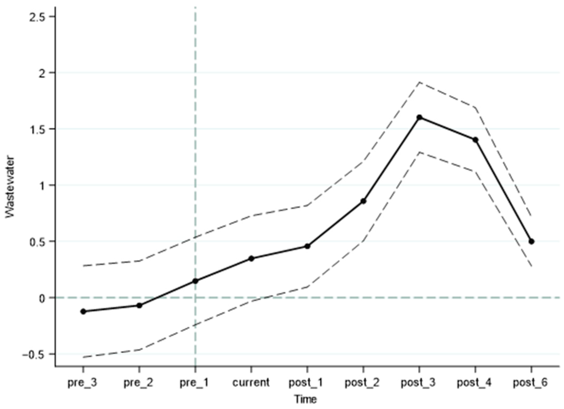
The premise of using the double-difference method is that the treatment group and the control group must satisfy the parallel trend test; that is, there must be significant difference in wastewater discharge between the treatment group and the control group before China’s accession to the WTO. In this paper, according to the event analysis method, time series dummy variables are set before 2001 and substituted into the model for regression. The specific results are shown in Figure 2. The difference between the treatment group and the control group is not significant before China’s accession to the WTO, and after China’s accession to the WTO, the treatment group shows a significant upward trend in wastewater discharge; therefore, the parallel trend test is passed. There is an obvious dynamic trend in the effect of trade liberalization on the pollution emissions of enterprises, and the coefficient begins to decline after the third period of China’s accession to the WTO, which may be related to the Chinese government’s increasing focus on the quality of economic growth and increasing environmental regulation.

4.2.2. Ex Ante Trend

The results of our parallel trend test do not necessarily guarantee that the treatment group is not systematically different from the control group. Therefore, to address potential endogeneity issues, the following analysis was conducted: we simulated trade liberalization at the prefecture level using 1990 industrial data and ran a regression. The results are shown in

Table 3. Ex ante trend.

VARIABLES	(1)
NTR•Post	−0.226
	(−0.64)
Scale	1.182 ***
	(116.13)
Ratio	−0.462 ***
	(−5.37)
HHI	1.559 ***
	(5.52)
CI	0.000
	(1.09)
Constant	2.362 ***
	(24.28)
Observations	266,153
R-squared	0.291
Industry FE	YES
Year#Pro FE	YES

Note: *** p < 0.01, t-statistics in parentheses, # represents joint fixed effects.

. The regression results are not significant, suggesting to some extent that the treatment and control groups are not different before the policy shock.

4.2.3. Elimination of Selection Bias

In the baseline regression process, since the division of the treatment and reference groups may not be randomly selected, and since the treatment and reference groups have different characteristics, this will cause “selectivity bias” in the double-difference method. This bias can lead to a correlation between the explanatory variables and the residuals, causing an endogeneity problem. To address this potential endogeneity problem, we used the PSM-DID method to obtain the average treatment effect. The first step is to match the propensity scores of the covariates to find a reference group that is as similar as possible to the treatment group, and then to obtain the average treatment effect of the policy impact through double-differencing, which makes the results more reliable. As shown in Panel A of

Table 4. PSM-DID.

Panel A
Matching Method	Treated	Control	Difference	t
One-to-one nearest neighbor matching	9.758	8.957	0.801	5.46
Panel B
NTR•Post		0.474 **
		(2.11)
Scale		1.135 ***
		(83.49)
Ratio		−0.408 ***
		(−3.67)
HHI		2.126 ***
		(3.25)
CI		−0.003 ***
		(−3.45)
Constant		2.476 ***
		(16.13)
Observations		104,984
R-squared		0.290
Industry FE		YES
City FE		YES
Year#Pro FE		YES

Note: *** p < 0.01, ** p < 0.05, t-statistics in parentheses, # represents joint fixed effects.

, we use one-to-one nearest neighbor matching to find that the difference between the treatment group and the control group is positive at the 1% significance level; secondly, we delete the treatment group and the control group that are not involved in the matching and regress them according to Model (1). As shown in Panel B of Table 4, the results are still robust. To ensure the validity of the PSM method, we subjected the samples to a parallel trend test after PSM, and as shown in Figure 3, the results showed that there was no significant difference between the treatment and control groups.

4.2.4. Adding Control Variables

Although we exclude interference from ex ante trends in the treatment and control groups, there is still interference from technological advances, environmental regulations, and other factors. Therefore, we further control for firm age, firm sales value, green patents in prefecture-level cities, non-agricultural population in prefecture-level cities, tertiary industry share in prefecture-level cities, and pollution emission compliance rate in prefecture-level cities. The results are shown in columns 1–2 of

Table 5. Adding control variables.

VARIABLES	(1)	(2)
NTR•Post	0.891 ***	0.859 ***
	(5.11)	(4.23)
Scale	0.849 ***	0.934 ***
	(49.98)	(38.29)
ratio	−0.606 ***	−0.822 **
	(−4.32)	(−2.35)
hhi5	−0.087	−1.079
	(−0.29)	(−1.29)
Capital	−0.001	−0.002
	(−1.32)	(−1.30)
Age	0.233 ***	0.243 ***
	(18.93)	(13.86)
Sale	0.314 ***	0.355 ***
	(24.55)	(18.96)
Green		-0.032
		(−1.25)
Non_agriculture		0.630 ***
		(3.48)
Third_ratio		−0.002
		(−0.22)
Enviromental regulation		−0.001
		(−1.45)
Constant	0.656 ***	−3.250 ***
	(5.22)	(−3.24)
Observations	174,311	108,987
R-squared	0.325	0.327
Industry FE	YES	YES
City FE	YES	YES
Year#Pro FE	YES	YES

Note: *** p < 0.01, ** p < 0.05, t-statistics in parentheses, # represents joint fixed effects.

, where the core explanatory variables remain significantly positive.

4.2.5. Placebo Test

In the model setting of this paper, the grouping of the treatment and control groups is based on the fact that tariffs on different industries decline to different degrees, and the existence of different time trends in the treatment group and the control group is due to the influence of trade expansion. If our grouping is not based on the fact that their tariffs fall to different degrees but is instead randomized, then, theoretically, there is no treatment effect. In view of this, we mix the treatment and control groups, employ random sampling to obtain a spurious treatment and control group, and run a regression analysis according to Equation (1). Repeating the above process 500 times, the extracted coefficients and p-values are shown in Figure 4, the average value of the spurious coefficients is 0, while the true value of the regression results in this paper is 0.713. At the same time, the p-values are mostly higher than 0.1, which proves that randomly switching the treatment group with the control group does not favor a significant difference, and further excludes other factors from interfering with the regression results.

4.2.6. Replacement Variables

This paper passes the parallel trend hypothesis and the placebo test, but a question of concern is whether trade liberalization has the same effect on other pollutants. Therefore, this paper chooses other major pollutants (industrial exhaust, sulfur dioxide, nitrogen oxide, chemical oxygen, and dust) for a robustness test, and the results are shown in columns 1–5 of

Table 6. Replacement variables.

VARIABLES	(1)	(2)	(3)	(4)	(5)
	Exhaust	SO2	Nitrogen Oxide	Chemical Oxygen	Dust
NTR•Post	0.422 ***	0.123	2.968 ***	0.660 ***	0.621 ***
	(3.10)	(0.69)	(17.54)	(3.75)	(3.57)
Scale	0.971 ***	0.874 ***	0.600 ***	1.203 ***	0.755 ***
	(108.85)	(76.92)	(44.47)	(118.75)	(67.79)
Ratio	−0.079	−0.103	−0.311***	−0.193 ***	0.040
	(−1.51)	(−1.48)	(−4.62)	(−3.54)	(0.70)
HHI	1.078 ***	2.713 ***	−0.933 **	−1.599 ***	0.022
	(4.08)	(8.18)	(−2.53)	(−5.32)	(0.07)
CI	−0.001 ***	0.000	0.005 ***	−0.002 ***	0.000
	(−2.85)	(1.16)	(32.06)	(−5.46)	(0.82)
Constant	1.154 ***	2.910 ***	3.701 ***	0.076	2.629 ***
	(14.54)	(28.32)	(37.84)	(0.78)	(25.77)
Observations	273,890	271,852	53,972	272,828	265,441
R-squared	0.371	0.313	0.285	0.392	0.280
Industry FE	YES	YES	No	YES	YES
City FE	YES	YES	YES	YES	YES
Year#Pro FE	YES	YES	YES	YES	YES

Note: *** p < 0.01, ** p < 0.05, t-statistics in parentheses, # represents joint fixed effects.

. The results show that trade liberalization also promotes the emission of other pollutants.

4.3. Mechanism Testing

4.3.1. External Factors

According to the theoretical analysis in the previous section, this paper supports the pollution paradise hypothesis based on the entry of foreign capital. The entry of foreign investment in China has a very obvious geographical characteristic, as shown in Figure 5a, which shows that foreign investment in China is mainly concentrated in the coastal areas. In addition, the most significant areas of industrial wastewater discharge in China are also concentrated in the coastal areas (see Figure 5b). This suggests that there may be a correlation between the entry of foreign investment and corporate pollution emissions.

In order to further demonstrate the research hypotheses of this paper in detail, we adopt a more rigorous empirical test to regress trade liberalization on the share of foreign investment of enterprises. Specific results are shown in column 1 of

Table 7. External factors.

VARIABLES	(1)	(2)	(3)	(5)	(6)
	Full Sample	High Pollution	Low Pollution	High Skill	Low Skill
NTR•Post	0.068 ***	0.053 ***	0.024	−0.095 **	0.085 ***
	(6.67)	(3.82)	(1.63)	(−2.38)	(7.65)
Scale	0.021 ***	0.019 ***	0.021 ***	0.020 ***	0.021 ***
	(24.71)	(15.11)	(18.93)	(9.29)	(22.01)
Ratio	0.007	−0.009	0.012 **	0.226 ***	−0.011 **
	(1.52)	(−1.17)	(2.54)	(10.21)	(−2.53)
HHI	−0.080 ***	−0.192 ***	0.899 ***	0.611 ***	−0.088 ***
	(−2.96)	(−5.20)	(14.25)	(6.16)	(−3.09)
Capital	−0.000 ***	−0.002 ***	−0.000 ***	0.000 **	−0.000 ***
	(−17.62)	(−14.92)	(−9.91)	(2.47)	(−17.03)
Constant	0.033 ***	0.163 ***	−0.102 ***	−0.046 *	0.033 ***
	(5.09)	(14.54)	(−9.25)	(−1.95)	(4.88)
Observations	291,043	144,627	146,414	50,896	240,144
R-squared	0.239	0.282	0.200	0.290	0.237
City FE	YES	YES	YES	YES	YES
Year#Pro FE	YES	YES	YES	YES	YES

Note: *** p < 0.01, ** p < 0.05, * p < 0.1, t-statistics in parentheses, # represents joint fixed effects.

. Trade liberalization significantly increases the share of foreign investment in Chinese enterprises. However, the relationship between trade liberalization and foreign investment entry alone cannot explain the pollution paradise or pollution halo hypotheses. Therefore, according to the General Office of the State Council on the issuance of the first national census of sources of pollution, the industry is divided into high-pollution and low-pollution industries to determine the entry of foreign investment. As shown in columns 2–3 of Table 7, more foreign capital enters into high-pollution industries. We further categorize the industries into technology-intensive and non-technology-intensive, and as shown in columns 4–5 of Table 7, the results show that China’s foreign investment is concentrated in low-technology sectors. It is inferred that China’s foreign investment structure is mainly composed of low-quality foreign investment. Therefore, Hypothesis 1 of this paper holds.

4.3.2. Internal Factors

Another mechanism of action in this paper suggests that firms have a strong profit motive to increase their energy consumption during trade expansion, which also increases firms’ pollution emissions. As shown in Column 1 of

Table 8. Internal factors.

VARIABLES	(1)	(2)	(3)	(4)
	Total	Coal	Oil	Gas
NTR•Post	0.396 ***	2.963 ***	−0.094	0.116 ***
	(3.82)	(25.23)	(−1.35)	(3.78)
Scale	1.074 ***	0.593 ***	0.357 ***	0.175 ***
	(111.39)	(55.87)	(41.17)	(28.13)
Ratio	−0.291 ***	−0.062	−0.025	−0.035 *
	(−3.66)	(−1.19)	(−0.86)	(−1.80)
HHI	6.239 ***	3.645 ***	−1.494 ***	−0.478 ***
	(21.48)	(13.14)	(−6.98)	(−3.97)
CI	0.010 ***	0.006 ***	0.004 ***	0.002 ***
	(49.93)	(32.10)	(20.71)	(17.12)
Constant	2.912 ***	−0.043	−1.398 ***	−0.967 ***
	(35.80)	(−0.56)	(−23.01)	(−20.34)
Observations	144,962	262,269	228,452	149,906
R-squared	0.281	0.226	0.234	0.260
City FE	YES	YES	YES	YES
Year#Pro FE	YES	YES	YES	YES

Note: *** p < 0.01, * p < 0.1, t-statistics in parentheses, # represents joint fixed effects.

, trade expansion increases the consumption of total energy and also significantly increases the consumption of coal and natural gas. Therefore, Hypothesis 2 of this paper holds.

5. Heterogeneity Analysis

5.1. Heterogeneity at the Firm Level

Since trade expansion, export has become one aspect of the troika driving China’s economic growth. According to the theory of heterogeneity [39], for exporting firms, the scale of production will be larger and energy consumption will be greater. On the other hand, foreign investors also see China as an important export base, and thus the share of foreign capital in exporting firms will be higher. Therefore, this paper hypothesizes that there is a significant difference in the level of wastewater discharge between exporting and domestic firms after trade expansion. The specific results are shown in columns 1–2 of

Table 9. Heterogeneity analysis.

VARIABLES	(1)	(2)	(3)	(4)	(5)	(6)
	Export	Domestic	Labor	Capital	Coastal	Non-Coastal
NTR•Post	1.044 ***	0.704 ***	0.851 ***	−2.303 ***	0.950 ***	0.426 **
	(3.71)	(3.60)	(4.34)	(−2.69)	(3.91)	(2.03)
Scale	1.139 ***	1.225 ***	1.005 ***	1.405 ***	0.919 ***	1.409 ***
	(81.57)	(93.81)	(74.94)	(103.86)	(61.89)	(107.80)
Ratio	−0.729 ***	−0.362 ***	−0.453 ***	−0.427 ***	−0.542 ***	−0.384 ***
	(−7.30)	(−4.20)	(−5.24)	(−3.78)	(−5.52)	(−4.14)
HHI	1.289 ***	1.243 ***	−0.668 *	−4.034 ***	0.118	0.305
	(3.05)	(3.25)	(−1.75)	(−4.03)	(0.32)	(0.71)
Capital	−0.000	0.000	0.007 ***	0.003 ***	−0.003 ***	0.002 ***
	(−0.52)	(0.97)	(3.54)	(4.77)	(−4.30)	(3.25)
Constant	2.609 ***	1.883 ***	2.760 ***	2.238 ***	4.827 ***	0.402 ***
	(18.16)	(15.93)	(18.03)	(7.03)	(35.63)	(3.17)
Observations	104,705	172,184	142,773	134,120	111,236	165,656
R-squared	0.341	0.314	0.300	0.369	0.287	0.338
Industry FE	YES	YES	YES	YES	YES	YES
City FE	YES	YES	YES	YES	YES	YES
Year#Pro FE	YES	YES	YES	YES	YES	YES

Note: *** p < 0.01, ** p < 0.05, * p < 0.1, t-statistics in parentheses, # represents joint fixed effects.

, where trade liberalization promotes wastewater discharge in exporting firms more than non-exporting firms.

5.2. Heterogeneity at the Industry Level

According to the theory of comparative advantage, China’s abundant and cheap labor force is one of the factors attracting foreign investment into the country. If foreign capital is the main mechanism behind trade expansion’s promoting of corporate pollution emissions, the level of pollution emissions in labor-intensive industries may be higher than that in capital-intensive industries. In this paper, the labor-to-capital ratio is divided into two groups, high labor and low labor, according to the median, which represent labor-intensive and capital-intensive industries, respectively. The specific results are shown in columns 3–4 of Table 9, where it is shown that trade liberalization promotes pollution emissions in labor-intensive industries more than in capital-intensive industries.

5.3. Heterogeneity Analysis at the Regional Level

According to the theory of locational advantage, foreign investment into China is more concentrated in coastal regions, mainly because coastal regions have better geographic locations and policy advantages compared to non-coastal regions. We thus hypothesize that trade liberalization has a greater effect on corporate pollution emissions in coastal areas (i.e., in Guangdong, Fujian, Zhejiang, Jiangsu, and Shanghai). The specific results are shown in columns 5–6 of Table 9, where trade liberalization is shown to produce a stronger effect on pollution emissions in coastal areas.

6. Further Analysis

6.1. Enterprise Migration

In this paper, the theoretical hypothesis mentions that differences in environmental standards between regions are one of the motivations for firms to relocate, and that the pollution haven hypothesis applies not only to firms’ location decisions at the international level, but also potentially for firms’ location decisions at the domestic, interregional level. According to the pollution paradise hypothesis, firms that move to areas with low environmental regulations are likely to have worse environmental performance than other relocating firms. In this paper, we statistically examine the spatial distribution of corporate pollution over the 1998–2007 period (as shown in Figure 6), and a certain spatial shifting is observed.

The model is further set to Equation (3) below, with Migration denoting the firms that undergo relocation during the sample period. In this paper, a change in a firm’s regional administrative code is regarded as a relocation during the sample period. The specific results are shown in columns 1–2 of

Table 10. Enterprise migration.

VARIABLES	(1)	(2)
	County	City
NTR•Post•Migration	0.088 ***	0.330
	(3.98)	(0.54)
Scale	1.210 ***	1.210 ***
	(120.27)	(120.27)
Ratio	−0.432 ***	−0.436 ***
	(−5.42)	(−5.44)
HHI	1.048 ***	1.354 ***
	(3.66)	(4.93)
CI	0.001	0.0003
	(1.36)	(0.80)
Constant	2.080 ***	2.208 ***
	(22.14)	(24.90)
Observations	276,893	276,893
R-squared	0.322	0.322
Industry FE	YES	YES
City FE	YES	YES
Year#Pro FE	YES	YES

Note: *** p < 0.01, t-statistics in parentheses, # represents joint fixed effects.

, where the migration of firms at the county level and at the prefecture level are both positive, indicating that under trade liberalization, firms are incentivized to relocate to avoid regulation. Hypothesis 3.1 of this paper therefore holds.

$$\ln pollutio{n}_{ijt}={\alpha }_0+{\alpha }_{1}NT{R}_j\times Pos{t}_t\times Migratio{n}_i+{\alpha }_3{X}_{ijt}+{\eta }_j+{\gamma }_s+{\lambda }_{ct }+{\xi }_{it}$$

(3)

6.2. Spatial Correlation

Under the premise of assumption 3.1, there may be local spillover and proximity effects from trade liberalization on the pollution emissions of enterprises. Therefore, we set up the following spatial Durbin model for regression analysis. In order to meet the data requirements of spatial measurement, we set all the explanatory and interpreted variables in Model (4) to the city level and selected the following control variables: the total population of the city (Population), the contribution of secondary industries to the GDP (Second ratio), the amount of investment in fixed assets (Investment), and the regional gross domestic product (GDP). All data are obtained from local statistical yearbooks.

$$\ln pollutio{n}_{ct}={\alpha }_{1}NT{R}_c\times Pos{t}_t+{\alpha }_{1}W\times NT{R}_c\times Pos{t}_t+{\alpha }_3{X}_{ct}+{\alpha }_{3}W\times X_{ct}+{\xi }_{ct}$$

(4)

where W denotes the spatial geographic weight matrix between cities, which takes into account that geographic location is the primary reason for spatial spillovers of economic activities. The closer the geographical distance, the higher the spatial correlation between individuals is likely to be. The specific results are shown in

Table 11. Spatial Durbin model.

VARIABLES	(1)	(2)
	Main	WX
NTR•Post	2.338 ***	15.696 **
	(5.34)	(2.34)
Population	0.445 ***	0.657
	(6.01)	(1.00)
Second ratio	2.590 ***	−3.515 *
	(7.53)	(−1.70)
Investment	0.030	−0.190
	(0.75)	(−0.43)
GDP	0.612 ***	−2.752 ***
	(7.90)	(−3.20)
Observations	2100	2100
R-squared	0.499	0.499
FE	YES	YES

Note: *** p < 0.01, ** p < 0.05, * p < 0.1, t-statistics in parentheses.

; the WX regression coefficients are significantly positive, indicating that trade liberalization in other regions significantly enhances the level of pollution emissions in the region, proving the existence of spatial spillover effects. Meanwhile, our decomposition of the total effect into direct and indirect effects similarly proves that the local pollution emission level is affected by trade expansion in other regions (as shown in

Table 12. Decomposition of effects.

VARIABLES	Total	Direct	Indirect
NTR•Post	96.985 *	2.806 ***	94.179 *
	(1.73)	(5.04)	(1.69)
Population	5.929	0.468 ***	5.461
	(1.47)	(6.66)	(1.35)
Second ratio	−5.746	2.572 ***	−8.319
	(−0.48)	(8.18)	(−0.69)
Investment	−0.628	0.026	−0.653
	(−0.26)	(0.64)	(−0.27)
GDP	0.555 ***	−12.277 *	−11.723
	(7.35)	(−1.71)	(−1.63)

Note: *** p < 0.01, * p < 0.1, t-statistics in parentheses.

). Hypothesis 3.2 is therefore proven.

To account for pollution spillovers from trade liberalization even further, we analyze the spatial distribution of polluting firms, which we measure using four-digit industry codes. The results, as shown in column 1 of

Table 13. Space threshold regression.

VARIABLES	(1)	(2)	(3)	(4)
	Total	100 km	200 km	300 km
NTR•Post	2.338 ***	28.193	33.871 *	57.939 ***
	(5.34)	(1.48)	(1.73)	(2.81)
Space spillover term
NTR•Post	94.1703 *	−20.599	−58.130	129.098 ***
	(1.79)	(−0.89)	(−1.08)	(3.34)
Observations	2100	2100	2100	2100
FE	YES	YES	YES	YES

Note: *** p < 0.01, * p < 0.1, t-statistics in parentheses.

, show that there are spatial spillover effects of trade liberalization on the distribution of polluting firms. This paper further analyzes the impact of spatial spillover effects on neighboring cities using a threshold spatial econometric model, and the results, as shown in columns 2–4 of Table 13, show that the spatial spillover effects start to appear at about 300 km from the central city, which proves that firms have a strong incentive to avoid environmental regulation and thus decide to relocate. The underlying logic of this result is that if firms are relocating for cost, then the closer they are, the more pronounced the spillovers are. However, the results of this paper show that reaching a distance of around 300 km is significant to some extent, suggesting speculative behavior by firms.

6.3. Corruption and Environmental Regulation

Hypotheses 3.1 and 3.2 demonstrate that there are spatial spillovers from firms’ pollution emissions, and that it is likely that firms relocate from regions with high environmental regulations to regions with low environmental regulations. The theoretical analysis in the previous section of this paper suggests that the “promotion tournament” unique to the Chinese government is likely to lead to rent-seeking by firms from government officials, which in turn generates negative environmental externalities. Based on the data from the local procuratorates, we analyzed the number of crimes committed by public officials in each region and divided them into two groups: high-corruption regions and low-corruption regions. The regression results are shown in columns 1–2 of

Table 14. Corruption and environmental regulation.

VARIABLES	(1)	(2)	(3)	(4)
	High Corruption	Low Corruption	High Regulation	Low Regulation
NTR•Post	0.942 ***	0.506 **	0.631 ***	1.038 ***
	(4.35)	(2.08)	(2.72)	(5.18)
Scale	1.221 ***	1.202 ***	1.279 ***	1.143 ***
	(91.62)	(84.87)	(97.34)	(95.31)
Ratio	−0.434 ***	−0.433 ***	−0.415 ***	−0.438 ***
	(−3.47)	(−4.68)	(−4.78)	(−3.07)
HHI	1.057 ***	0.636	−1.359 ***	2.306 ***
	(2.70)	(1.53)	(−3.13)	(6.46)
Capital	−0.000	0.002 ***	0.004 ***	−0.001 *
	(−0.73)	(2.79)	(6.67)	(−1.72)
Constant	2.113 ***	2.036 ***	1.260 ***	2.701 ***
	(16.21)	(15.50)	(9.60)	(23.07)
Observations	140,367	136,525	135,686	141,207
R-squared	0.302	0.346	0.343	0.298
Industry FE	YES	YES	YES	YES
City FE	YES	YES	YES	YES
Year#Pro FE	YES	YES	YES	YES

Note: *** p < 0.01, ** p < 0.05, * p < 0.1, t-statistics in parentheses, # represents joint fixed effects.

, which show that trade liberalization in high-corruption regions leads to higher pollution emissions from firms, highlighting the decline in environmental governance capacity brought about by corruption. Hypothesis 4.1 of this paper is therefore proven. The government’s ability to govern the environment has always been a matter of public concern, especially concerning what approach to take to gain more value from the discussion. The theoretical analysis of this paper has shown that command-type environmental regulations often take a one-size-fits-all approach to environmental governance, ignoring the reality of the production and operation of enterprises and pertinent industry characteristics, often producing the opposite results. Therefore, it is worth testing whether a softer market-based environmental regulation approach can achieve better governance results. To this end, we measure the government’s level of environmental regulation by the amount of government investment in pollution control/industrial value added, which is divided into a high environmental regulation group and a low environmental regulation group. The specific results, as shown in columns 3–4 of Table 14, show that the government can effectively curb the environmental pollution problem accompanying trade expansion by strengthening its investment in environmental governance. Hypothesis 4.2 of this paper therefore holds.

7. Conclusions

This paper empirically examines the relationship between trade expansion and industrial wastewater emissions of Chinese enterprises based on the micro-database of enterprises in China. The following conclusions are obtained. First, trade expansion boosts firms’ industrial wastewater emissions; specifically, each unit of tariff decline leads to a 0.713 percentage point increase in the growth rate of wastewater emissions, and trade expansion also has a boosting effect on the emissions of major pollutants (industrial exhaust, sulfur dioxide, nitrogen oxide, chemical oxygen, and dust). The mechanism of action suggests that, considering the external factors, trade expansion allows for the entry of low-quality foreign capital support into China, establishing the pollution paradise hypothesis; regarding the internal factors, the huge external demand brought about by trade expansion stimulates the energy consumption of enterprises and thus raises their pollution emission levels. Heterogeneity analysis shows that trade expansion results in export enterprises, labor-intensive industries, and enterprises in coastal areas emitting higher levels of pollution, which is consistent with the theoretical analysis framework of this paper. A point of contribution of this paper compared to previous studies is that we found that there is a spatial spillover effect of trade liberalization on corporate pollution. Due to the different levels of environmental regulation and corruption across regions, the level of trade liberalization in neighboring regions also positively affects pollution emissions in the studied region. Therefore, strengthening environmental regulation and reducing corrupt rent-seeking can effectively curb the environmental costs of trade liberalization.

In addition to further enriching the pollution paradise hypothesis theoretically, this paper also has very important policy implications for the high-quality development of China’s economy.

7.1. Attracting High-Quality Foreign Investment

To attract high-quality foreign investment, the opening up of the service industry should be promoted, and foreign-invested enterprises should be encouraged to set up R&D centers to undertake major scientific research projects. Furthermore, lowering the entry thresholds for high-tech industries and facilitating the immigration of people from abroad would be beneficial. At the same time, there is a need for interregional FDI linkages to prevent a gradient shift in low-quality FDI between regions.

7.2. Developing the New Energy Industry

Increasing the synergistic support regarding taxes, land, financing, and talent would benefit the development of a new energy industry. Establishing a green credit fund and accelerating the creation of standards, certifications, and testing systems to guide and standardize the development of the industry are also recommended.

7.3. Market-Based Environmental Regulation

If administrative orders are used to intervene with industry, there will be spillover effects of environmental pollution. Therefore, governments need to develop market-oriented environmental regulatory strategies, such as subsidizing corporate environmental investments and promoting environmental market transactions among enterprises. At the same time, a unified enterprise emissions monitoring platform should be established between regions to prevent transfers of pollution.

References

- Jayachandran, S. How Economic Development Influences the Environment. Annu. Rev. Econ. 2022, 14, 229–252. [Google Scholar] [CrossRef]
- Fayiga, A.O.; Ipinmoroti, M.O.; Chirenje, T. Environmental Pollution in Africa. Environ. Dev. Sustain. 2018, 20, 41–73. [Google Scholar] [CrossRef]
- Yu, Y.; Li, K.; Duan, S.; Song, C. Economic Growth and Environmental Pollution in China: New Evidence from Government Work Reports. Energy Econ. 2023, 124, 106803. [Google Scholar] [CrossRef]
- He, Q. Fiscal Decentralization and Environmental Pollution: Evidence from Chinese Panel Data. China Econ. Rev. 2015, 36, 86–100. [Google Scholar] [CrossRef]
- Jiang, Y.; Wu, Q.; Brenya, R.; Wang, K. Environmental Decentralization, Environmental Regulation, and Green Technology Innovation: Evidence Based on China. Environ. Sci. Pollut. Res. 2023, 30, 28305–28320. [Google Scholar] [CrossRef]
- Zhang, Y.; Cui, X.; Liu, L. Environmental Regulation, Green Technology Progress and Haze Reduction and Carbon Reduction. Environ. Sci. Pollut. Res. 2023. [Google Scholar] [CrossRef] [PubMed]
- Eaton, J.; Kortum, S. Technology, Geography, and Trade. Econometrica 2002, 70, 1741–1779. [Google Scholar] [CrossRef]
- Caliendo, L.; Parro, F. Estimates of the Trade and Welfare Effects of NAFTA. Rev. Econ. Stud. 2015, 82, 1–44. [Google Scholar] [CrossRef]
- Winters, L.A.; McCulloch, N.; McKay, A. Trade Liberalization and Poverty: The Evidence So Far. J. Econ. Lit. 2004, 42, 72–115. [Google Scholar] [CrossRef]
- Chen, K.; Liu, X. Does Import Trade Liberalization Affect Youth Human Capital Accumulation: Evidence from Prefecture-Level Cities in China. Int. Rev. Econ. Financ. 2024, 91, 1084–1094. [Google Scholar] [CrossRef]
- Chao, C.-C.; Ee, M.S.; Nguyen, X.; Yu, E.S.H. Trade Liberalization, Firm Entry, and Income Inequality. Rev. Int. Econ. 2019, 27, 1021–1039. [Google Scholar] [CrossRef]
- Eskeland, G.S.; Harrison, A.E. Moving to Greener Pastures? Multinationals and the Pollution Haven Hypothesis. J. Dev. Econ. 2003, 70, 1–23. [Google Scholar] [CrossRef]
- Antweiler, W.; Copeland, B.R.; Taylor, M.S. Is Free Trade Good for the Environment? Am. Econ. Rev. 2001, 91, 877–908. [Google Scholar] [CrossRef]
- Kellenberg, D.K. A Reexamination of the Role of Income for the Trade and Environment Debate. Ecol. Econ. 2008, 68, 106–115. [Google Scholar] [CrossRef]
- Shapiro, J.S.; Walker, R. Why Is Pollution from US Manufacturing Declining? The Roles of Environmental Regulation, Productivity, and Trade. Am. Econ. Rev. 2018, 108, 3814–3854. [Google Scholar] [CrossRef]
- Wu, S.; Wei, T.; Qu, Y.; Xue, R.; Wang, H.; Shan, Y. How Does Global Value Chain Embeddedness Affect Environmental Pollution? Evidence from Chinese Enterprises. J. Clean. Prod. 2024, 434, 140232. [Google Scholar] [CrossRef]
- Gutiérrez, E.; Teshima, K. Abatement Expenditures, Technology Choice, and Environmental Performance: Evidence from Firm Responses to Import Competition in Mexico. J. Dev. Econ. 2018, 133, 264–274. [Google Scholar] [CrossRef]
- Cherniwchan, J. Trade Liberalization and the Environment: Evidence from NAFTA and U.S. Manufacturing. J. Int. Econ. 2017, 105, 130–149. [Google Scholar] [CrossRef]
- He, L.-Y.; Wang, L. Import Liberalization of Intermediates and Environment: Empirical Evidence from Chinese Manufacturing. Sustainability 2019, 11, 2579. [Google Scholar] [CrossRef]
- Bloom, N.; Genakos, C.; Martin, R.; Sadun, R. Modern Management: Good for the Environment or Just Hot Air? Econ. J. 2010, 120, 551–572. [Google Scholar] [CrossRef]
- Bustos, P. Trade Liberalization, Exports, and Technology Upgrading: Evidence on the Impact of MERCOSUR on Argentinian Firms. Am. Econ. Rev. 2011, 101, 304–340. [Google Scholar] [CrossRef]
- Shapiro, J.S. Trade Costs, CO2, and the Environment. Am. Econ. J. Econ. Policy 2016, 8, 220–254. [Google Scholar] [CrossRef]
- Duan, Y.; Jiang, X. Temporal Change of China’s Pollution Terms of Trade and Its Determinants. Ecol. Econ. 2017, 132, 31–44. [Google Scholar] [CrossRef]
- Prell, C.; Feng, K.; Sun, L.; Geores, M.; Hubacek, K. The Economic Gains and Environmental Losses of US Consumption: A World-Systems and Input-Output Approach. Soc. Forces 2014, 93, 405–428. [Google Scholar] [CrossRef]
- Peng, S.; Zhang, W.; Sun, C. ‘Environmental Load Displacement’ from the North to the South: A Consumption-Based Perspective with a Focus on China. Ecol. Econ. 2016, 128, 147–158. [Google Scholar] [CrossRef]
- He, L.-Y.; Huang, G. Are China’s Trade Interests Overestimated? Evidence from Firms’ Importing Behavior and Pollution Emissions. China Econ. Rev. 2022, 71, 101738. [Google Scholar] [CrossRef]
- Copeland, B.R.; Taylor, M.S. North-South Trade and the Environment*. Q. J. Econ. 1994, 109, 755–787. [Google Scholar] [CrossRef]
- Chichilnisky, G. North-South Trade and the Dynamics of Renewable Resources. Struct. Chang. Econ. Dyn. 1993, 4, 219–248. [Google Scholar] [CrossRef]
- Cole, M.A.; Elliott, R.J.R.; Okubo, T. International Environmental Outsourcing. Rev. World Econ. 2014, 150, 639–664. [Google Scholar] [CrossRef]
- Levitt, C.J.; Saaby, M.; Sørensen, A. The Impact of China’s Trade Liberalisation on the Greenhouse Gas Emissions of WTO Countries. China Econ. Rev. 2019, 54, 113–134. [Google Scholar] [CrossRef]
- Gumilang, H.; Mukhopadhyay, K.; Thomassin, P.J. Economic and Environmental Impacts of Trade Liberalization: The Case of Indonesia. Econ. Model. 2011, 28, 1030–1041. [Google Scholar] [CrossRef]
- Ederington, J.; Levinson, A.; Minier, J. Trade Liberalization and Pollution Havens. Adv. Econ. Anal. Policy 2004, 4. [Google Scholar] [CrossRef]
- Zhao, H.; Li, Y.; Wang, Z.; Zhao, R. Trade Liberalization, Regional Trade Openness Degree, and Foreign Direct Investment:Evidence from China. Emerg. Mark. Rev. 2024, 59, 101103. [Google Scholar] [CrossRef]
- Aizenman, J.; Noy, I. FDI and Trade—Two-Way Linkages? Q. Rev. Econ. Financ. 2006, 46, 317–337. [Google Scholar] [CrossRef]
- Humphrey, J.; Schmitz, H. How Does Insertion in Global Value Chains Affect Upgrading in Industrial Clusters? Reg. Stud. 2002, 36, 1017–1027. [Google Scholar] [CrossRef]
- Arkolakis, C.; Ramondo, N.; Rodríguez-Clare, A.; Yeaple, S. Innovation and Production in the Global Economy. Am. Econ. Rev. 2018, 108, 2128–2173. [Google Scholar] [CrossRef]
- Wang, D.T.; Chen, W.Y. Foreign Direct Investment, Institutional Development, and Environmental Externalities: Evidence from China. J. Environ. Manag. 2014, 135, 81–90. [Google Scholar] [CrossRef] [PubMed]
- Allcott, H.; Greenstone, M. Is There an Energy Efficiency Gap? J. Econ. Perspect. 2012, 26, 3–28. [Google Scholar] [CrossRef]
- Melitz, M.J. The Impact of Trade on Intra-Industry Reallocations and Aggregate Industry Productivity. Econometrica 2003, 71, 1695–1725. [Google Scholar] [CrossRef]
- Martin, R.; Muûls, M.; de Preux, L.B.; Wagner, U.J. Anatomy of a Paradox: Management Practices, Organizational Structure and Energy Efficiency. J. Environ. Econ. Manag. 2012, 63, 208–223. [Google Scholar] [CrossRef]
- Aitken, B.J.; Harrison, A.E. Do Domestic Firms Benefit from Direct Foreign Investment? Evidence from Venezuela. Am. Econ. Rev. 1999, 89, 605–618. [Google Scholar] [CrossRef]
- Chen, X.; Shao, Y.; Zhao, X. Does Export Liberalization Cause the Agglomeration of Pollution? Evidence from China. China Econ. Rev. 2023, 79, 101951. [Google Scholar] [CrossRef]
- Wu, H.; Guo, H.; Zhang, B.; Bu, M. Westward Movement of New Polluting Firms in China: Pollution Reduction Mandates and Location Choice. J. Comp. Econ. 2017, 45, 119–138. [Google Scholar] [CrossRef]
- Zhang, H.-Z.; He, L.-Y.; Zhang, Z. Can Policy Achieve Environmental Fairness and Environmental Improvement? Evidence from the Xin’an River Project in China. J. Policy Model. 2024, 46, 212–234. [Google Scholar] [CrossRef]
- Krugman, P. Increasing Returns and Economic Geography. J. Polit. Econ. 1991, 99, 483–499. [Google Scholar] [CrossRef]
- Li, H.; Zhou, L.-A. Political Turnover and Economic Performance: The Incentive Role of Personnel Control in China. J. Public Econ. 2005, 89, 1743–1762. [Google Scholar] [CrossRef]
- Zhou, Z.; Han, S.; Huang, Z.; Cheng, X. Anti-Corruption and Corporate Pollution Mitigation: Evidence from China. Ecol. Econ. 2023, 208, 107795. [Google Scholar] [CrossRef]
- Petroni, G.; Bigliardi, B.; Galati, F. Rethinking the Porter Hypothesis: The Underappreciated Importance of Value Appropriation and Pollution Intensity. Rev. Policy Res. 2019, 36, 121–140. [Google Scholar] [CrossRef]
- Erten, B.; Leight, J. Exporting Out of Agriculture: The Impact of WTO Accession on Structural Transformation in China. Rev. Econ. Stat. 2021, 103, 364–380. [Google Scholar] [CrossRef]
Figure 1.
Trends in China’s exports.