1. Introduction
The growing global commitment to sustainable energy, marked by an interest in generating electricity through renewable sources without contributing to greenhouse gas emissions, has brought to the forefront the increasing prominence of photovoltaic (PV) systems in the renewable energy landscape. This prominence underlines the importance of understanding and mitigating factors that can impact the performance of PV systems. As urban development rises, the variation in building heights has become particularly pronounced, especially in densely developed areas worldwide. According to an article published by the United Nations in 2018 [
1], urban areas are projected to accommodate 68% of the world’s population by 2050, emphasizing the significance of addressing shading issues in PV systems within urban environments. Consequently, the growing number of households per square area necessitates the installation of additional utility services on roof spaces to meet the increasing demand. These factors have led to distinctively aggravated shading issues for both existing and potential roof-mounted PV systems.
Ongoing advancements in PVs aim for an economically feasible efficiency limit of 29.43% in undoped crystalline silicon [
2], emphasizing the importance of addressing even minimal shading instances to avoid energy harvesting inefficiencies. Since the inception of PVs, extensive research has delved into investigating the effects of shading on PV systems. These research studies have led to PV systems being fitted with bypass diodes to mitigate the effect of shade mismatch, MPPT trackers to reduce the repercussions of shade on multiple modules, and wiring reconfigurations to avoid multiplication of the energy lost on other modules [
3,
4,
5]. While these mitigation measures have been proven to be vital solutions to the shading effect on PV systems, the studies that delve deep into these three main components primarily focus on the partial shading caused by hard, peripherally defined shadows such as walls and buildings. As elucidated by [
6], this constitutes just one aspect of partial shading. Moreover, researchers such as [
7,
8] employ simulation tools to replicate PV shading, affirming the effectiveness of innovative algorithms and electrical circuit devices similar to those outlined in [
9,
10].
Although studies using simulation tools yield commendable conclusions, it is evident that these simulation tools depend on manually adjusted predictors, such as irradiance levels in 100 W/m
2 increments and covering percentages of the PV module area in 25% intervals [
11,
12]. Significant outcomes are seen in outdoor conditions. When a section of the PV module is covered to simulate single-intensity hard shading, the findings reveal power losses of 99.36%, 43.7%, and 41.15% for shading extents of 75%, 50%, and 25% respectively [
13]. Nonetheless, the variation in shadow formation for soft shadows cast by thin objects tends to result in a distinct pattern of shadow formation and transposition on a PV source [
14,
15]. The presence of penumbra highlighted by [
16] shows that thin objects have different optical properties, and their impact depends on the distance between the PV source and the thin object. When compared to hard shading, the intensity is evidently depicted as consistent and can be regarded as a constant umbra shadow. Therefore, given the evident differences in shadow properties caused by shading, it becomes apparent that the standard simulation models utilized by PVSyst version 7.4, MATLAB version R2023a, and PVSol version 2023 R1 prove inadequate in accurately portraying shadow formation when assessing the resulting power loss from thin object shading. These simulations, restricted to single-intensity shadows, currently lack the capability to model precise shadow formations, thereby overlooking the coexistence of umbra and penumbra shadows in a single shadow formation [
17].
In a detailed examination of shadow formation, ref. [
16] demonstrates the optical principle inherent in a typical shadow formation, distinguishing the umbra as the central dark shade and the penumbra as the lighter shadow on the periphery. The existence of the penumbra, as highlighted by [
16], shows evidence that other types of partial shading, such as those transposed by thin objects, possess distinct optical properties, thus affecting the intensity of the shadow. This stands in contrast to hard shading, in which the shadow intensity remains relatively consistent and can be regarded as a constant umbra shadow [
14]. Among the limited number of research studies addressing thin object shading, Sinapis et al. [
15] conducted experiments simulating pole shading by covering 1% to 2% of the PV system surface to assess its performance under partial shading conditions. A significant 30–50% reduction in energy generation was observed when the thin pole was located at a distance of 69 cm from the PV module. Similarly, Dolara et al. [
18] observed significant power fluctuations caused by a medium voltage (MV) overhead line shading a large PV plant. The empirical data obtained from this investigation allowed Dolara et al. to consider relocating the position of the MV line to minimize shading impacts over the PV system’s operational lifetime. Notably, in the latter work, the authors did classify shading into umbra and penumbra; however, while the distance was mentioned, no correlation with shadow intensity was conducted. Therefore, there is a lack of empirical evidence demonstrating how power loss varies at various distances from the pole and MV power line. Contrastingly, Feng et al.’s study [
16] reported that when a 10 m pole was positioned farther away from the original setup that resulted in a 9.21% power loss, a drastic drop in power of between 2% and 5% was observed, meaning that when moved further away, the thin object shadow reduced its impact on the generation of the PV system. While there is substantial understanding of umbra and penumbra shading, only a limited number of researchers have undertaken the initiative to differentiate between these two shading formations.
Notably, refs. [
12,
19,
20] depict partial shading as hard shading based on percentage coverage, despite the use of a solar simulator that aims to mimic real conditions in a laboratory setting. Moreover, it is apparent that while the experimental setup significantly influences a comprehensive analysis of shadow effects, researchers commonly employ non-realistic methods to simulate shading. In contrast, Demouth et al. [
21], in a more thorough examination of shading properties, showcase a profound understanding of shadow dispersion. The study illustrates that as the height of an opaque object increases from a flat plane, the penumbra shadow becomes lighter but increases in overall size. However, while this phenomenon aligns with the fundamental principles of optical physics [
22], its implications in the context of shading on a PV source remain unclear. Additionally, it is unclear whether the increase in shadow size, i.e., when the thin object is farther away from the PV source, directly compensates for the reduced shadow intensity when analyzing the resultant power loss. In this regard, the primary predictors of power loss when a thin object casts a shadow near a PV source could be classified into two categories: object size, which is the more explored variable in research, and distance, which affects shadow intensity. Furthermore, to the best of our knowledge, in this field of study, the analysis of the penumbra shadow in isolation has yet to be undertaken to ascertain its true significance when cast upon a PV source.
Based on the literature reviewed above, two primary research gaps have been identified. First, the prevailing trend in most studies involves treating thin object shading with the same optical attributes of shadows cast by large objects transposing hard shading without considering the variable shadow intensity. The second research gap pertains to the methodological approach adopted for the analysis of thin object shading. Although outdoor experimentation and laboratory solar simulators have each shown their ability to produce satisfactory results as separate methods, there remains a significant gap in knowledge regarding comparative efficacy. Specifically, the question of how laboratory-based experimentation results fare in comparison to outdoor environmental experimentation remains, particularly in the context of analyzing thin object shading. Furthermore, the primary aim of this study is to determine the optimal ratio between object thickness and distance, where the impact on the performance of the PV system is minimal. While previous research has proposed various solutions such as power optimizers and MPPT trackers, this study endeavors to comprehensively understand the effects of thin object shading in terms of both thickness and distance on PV system performance; prioritizing efficient planning strategies under conditions of thin object shading is also deemed important. Moreover, the innovation showcased in this research stems from its unique way of integrating the optical shadow formation principles into the realm of photovoltaics. This study not only quantifies power loss on PV sources but also offers a graphical comparative representation of the evolving shadow formations as power loss fluctuates due to the shading effects of thin objects. This dual approach provides an understanding of shadow behavior under varying conditions, spanning both real-world environments and controlled laboratory settings.
2. Methodology
The methodology in this study is divided into two key approaches. First, outdoor experimental data was collected to emulate real-world conditions. Second, a laboratory-based solar simulator was used to conduct controlled experiments. This dual-method approach aimed to comprehensively investigate the shading effects on PV sources and provide a well-rounded analysis.
2.1. Outdoor Experimentation Methodology
First, to establish an authentic outdoor environment, the experiments were conducted outdoors at the Institute of Sustainable Energy situated in Marsaxlokk, Malta, at latitude 35.84117 and longitude 14.53931. These experiments aimed to quantify the impact of shading from thin objects of various sizes and positioned at different distances from the PV source. The experiments were conducted during the month of April in favorable weather conditions comprised of clear skies with no partial shading from clouds. Moreover, this research acknowledges the dynamic nature of solar positioning and its consequential impact on shadow projection. Due to the fact that the sun’s position changes continuously throughout the day and influences the size of shadows cast, an approach to address this variability in our experimentation was employed. Altitudes were generated at 15-minute intervals during our study, and trigonometric principles were applied to derive the apparent shadow transposed at various times of the day. Discrepancies between the shadow sizes observed at solar noon and other times of the day were rectified through the application of a correction factor to ensure a fair and standardized evaluation across different solar positions, as seen in
Figure 1 and the workings in
Table 1. Incorporating these considerations allowed the outdoor experimentation to maintain consistency and accuracy in the resultant power loss assessments, facilitating a comprehensive understanding of the dynamics between solar positioning, shadow projection, and power loss. Moreover, the setup consisted of two one-diode bypass monocrystalline PV modules (ET Solar model ET-M53620 sourced from Nanjing, China) rated at an output of 20 watts each with further specifications shown in
Table 2. One of the PV modules was used as the shaded module while the other module served as an unshaded control unit throughout the experiment.
To obtain the required data from the PV modules under experimentation, a custom-built circuit board was wired according to the specifications of the data logger DATAQ DI-808. Subsequently, the
Vmp was recorded at a very high accuracy (±0.05% of span + 10 μV) through a fixed resistive load while the
Imp was retrieved by measuring the voltage drop through a high-quality aluminum wire wound shunt resistor, both of which were mounted on an aluminum heat sink to dissipate heat and reduce errors. The schematic upon which the experimentation was conducted can be seen in
Figure 2. In this way, the experimental circuit box was capable of measuring both voltage and current, enabling the calculation of the maximum power (
Pmax) by multiplying
Imp with
Vmp. Consequently, using Equation (1), the power loss could be determined.
A calibration procedure was conducted by using the control PV as a baseline to determine the differentiating factor between the two PV modules under testing, despite their identical specifications. This involved obtaining current and voltage readings at intervals of 1 s for 15 min to derive a mismatch factor representing the difference in electrical outputs between both PV modules of the same cell type. This approach ensured the initialization of the experimentation at the same baseline electrical outputs at an accuracy of ±0.1%. Because this research paper addresses the research gap of the significance of the effect of distance and object thickness as predictors of thin object shading, a custom steel structure was built to vary the distance between the PV module and the thin object transposing shading. The chosen setup is depicted by the conceptual drawing in
Figure 3 and the actual structure in
Figure 4. The structure was capable of varying the distance between the PV module and the thin object between 25 cm and 250 cm, at increments of 25 cm. In order to address the identified research gap related to object thicknesses, this study also considered a variety of different thin objects with the following thickness: 2, 2.3, 2.8, 3.2, 3.4, 4.4, 4.6, 6, 6.4, 7.2, 8, 10, 12, 14, and 20 mm.
It is important to note that although there was no partial shading from objects when conducting our experiments on a sunny day, the nature of the light source cannot be solely attributed to direct radiation [
23]. Therefore, our experimentation assumes a blend of direct and diffused radiation while disregarding ground reflection due to the PV module’s direct orientation toward the sky at a 0-degree tilt angle [
24]. To ensure accuracy, the corrected irradiance level was measured at a weather station approximately 10 m from the experimental setup location. The procedure and basic measuring requirements for conducting the experimentation in this section are based on IEC 60904-1:2020 ‘Photovoltaic devices—Part 1: Measurement of photovoltaic current-voltage characteristics’ [
25]. The data retrieved from the data logger at operating conditions was baselined to the standard test conditions (STC) of 25 °C and 1000 W/m
2 (Air Mass 1.5G) irradiance to compare the shaded and unshaded PV module irrespective of the on-site temperature and irradiance [
26]. This procedure was conducted using the second procedure listed in [
27] IEC 60891:2021 consisting of correction parameters of the PV module for current and voltage, which are listed as Equations (2) and (3), respectively. Moreover, to further enhance the reputability of the data, the experiments were repeated three times, and the results were averaged to derive a representative reading for each combination of distance and thickness.
where:
I1 and V1 refer to current and voltage measured at operating conditions (OPC);
I2 and V2 refer to current and voltage measured at STC conditions;
G1 is the irradiance measured at OPC conditions;
G2 is the standard irradiance (1000 W/m2);
T1 is the cell temperature measured at OPC conditions;
T2 is the standard cell temperature (25 °C);
Voc1 is the open circuit voltage at OPC conditions;
αrel and βrel are, namely, the current and voltage temperature coefficients of the test specimen measured at 1000 W/m2;
a is the irradiance correction factor for the open circuit voltage;
Rs′ is the internal series resistance of the test specimen; and
k′ is the temperature coefficient of the internal series resistance
Rs′ [
28].
2.2. Laboratory Experimentation Methodology
In the second segment of the employed methodology, laboratory experimentation served the purpose of establishing a controlled environment for measuring the power output of raw, unencapsulated PV cells under various shading scenarios. In contrast to the outdoor experimentation, raw unencapsulated PV cells were chosen as the PV source to align with the rigging specifications of the Photo Emission Tech., Inc. (Moorpark, CA, USA). A solar simulator (SS150AAA–EM), situated at the Solar Research Laboratory at the Institute for Sustainable Energy, University of Malta, was also used. The solar simulator interfaces with an I-V tester measurement system Advance CC Series Model and is proficient in measuring parameters such as Pmax, Vmp, Imp, Voc, Isc, and cell efficiency. For data acquisition in this research, the focus was directed toward the Vmp, Imp, and Pmax of the unencapsulated solar cell under testing. The procedure and measurement requisites in this section adhere to the standard IEC 60904-1:2020.
Before initiating daily testing, the solar simulator underwent calibration using the reference cell Model 60623 PET Serial RC-1160 (Moorpark, CA, USA), ensuring a constant irradiance value of 1000 W/m
2 ± 1%. Additionally, a Peltier cell temperature control device was employed to maintain a consistent temperature of 25 °C for the solar cell being tested. These standardized experimental configurations allowed for baseline results under STC conditions, ensuring a fair and consistent basis for comparison. The experiment featured one monocrystalline solar cell, with detailed specifications shown in
Table 3, to provide the current and voltage values and enable a direct comparison of performance within the experimental conditions.
A specialized, small-scale variable structure was custom-built to manipulate the positioning of thin objects, as illustrated in
Figure 5. The methodology, however, encountered a limitation with a capped distance of 40 cm between the individual PV cell and the light source due to the physical constraints of the equipment. Moreover, all thin objects from the outdoor experimentation, along with the calibration procedure, were retained. The only exception was the shaded PV module being systematically compared with the unshaded data after each experimentation round rather than instantaneously, aligning with the limitations of the setup.
Under the solar simulator’s radiant illumination, the various-sized thin objects were methodically positioned individually until every possible combination of distance and thicknesses was covered. Upholding the principles of reliability and comprehensiveness, the experimental procedure underwent three iterations. This repetitive approach sought to establish the repeatability of outcomes and generate a more comprehensive dataset of power loss figures for each unique scenario.
An integral aspect of the experimental methodology involved the systematic capture of images for each combination of rod thickness and distance. This documentation serves a dual purpose: First, it is able to interpret specific discrepancies between outdoor and laboratory experimentation, providing visual insights into the effects of shading under varying conditions. Second, the images serve as crucial visual aids in illustrating the dynamic changes in shadow formations resulting from different distances and object thicknesses. Moreover, each image was manually examined to determine the estimated size of total shadow, as well as the approximate umbra and penumbra shadows as a percentage of the total area of the PV source, respectively.
3. Results and Discussion
The results section is comprised of two parts: outdoor experimentation analysis investigating thin object shading effects in natural conditions and laboratory experimentation using a solar simulator to explore controlled environmental impacts on PV performance. These sections collectively provide an understanding of thin object shading in diverse experimental settings.
3.1. Outdoor Experimentation Analysis
In the initial phase of the experiment, the focus was on obtaining an image dataset in order to understand the dynamics of shadow formation in various combinations of object thickness and distance from the PV source. The experimental process involved the systematic capture of images using a high-quality single-lens reflex (SLR) camera across all relevant configurations. Consistent camera settings were maintained for both outdoor and indoor experimentation to establish a level playing field across the two scenarios. These settings remained uniform throughout the study, ensuring baseline consistency and minimizing variability in image acquisition. Specifically, the camera settings included a film speed (ISO) of 200, an aperture of f/4, and a shutter speed of 1/125. These parameters were selected to optimize image quality and maintain uniformity across different experimental conditions. By adhering to consistent camera settings, variations in image quality attributable to technical factors were minimized, enabling a fair comparison of results across the study’s diverse scenarios.
Figure 6 presents these configurations with a specific emphasis on the 6 mm rod as an illustrative example. These images serve as a visual relation to the findings of the evolving shadow characteristics.
The five comparative graphs illustrated in
Figure 7 depict the relationship of the percentage of power loss and the object thickness with distance while simultaneously portraying the correlation with the approximate total shadow and its subsets, namely, umbra and penumbra. Notably, the results reveal a noticeable pattern wherein an increase in object thickness correlates with a proportional increase in power loss. Specifically, the power loss steadily rises, nearing 35% with a 20 mm rod, while a 2 mm rod yields a relatively modest 4% power loss. Furthermore, the examination of the total shadow indicates a consistent growth at a 50 cm distance, but this effect diminishes as the distance extends up to 250 cm, plateauing around a 10 cm thickness. Further analysis on the individual contributions of the umbra and penumbra shows that up to a distance of 100 cm, the percentages of umbra and penumbra closely align, with the exception of thicker-shading objects. Furthermore, beyond the 100 cm distance, a notable trend emerges in which the umbra experiences a sharp decline, while the penumbra compensates for this reduction. Drawing on insights from the literature review presented earlier in this research paper in which the penumbra is established as casting a lower-intensity shadow compared to the umbra, the current findings validate this notion. Consequently, although the overall trend in total shadow remains relatively consistent beyond a distance of 50 cm, the concurrent increase in the penumbra and decrease in the umbra result in a lower rate of power loss.
From here onward, the effect and relation will be assessed with the aid of the p-value, which serves as a measure of the strength of evidence supporting the observed. A smaller p-value signifies a higher statistical significance between the considered factors.
The data from the outdoor experimentation were analyzed using a bivariate correlation analysis through IBM® SPSS®, revealing a highly significant impact of the umbra on power loss indicated by a p-value of less than 0.001. This highlights the important role of the umbra in influencing power loss. On the other hand, despite the penumbra exhibiting higher percentage rates beyond a distance of 50 cm, its correlation with power loss is statistically insignificant when the umbra is considered simultaneously, with a p-value exceeding 0.05. This suggests that while the penumbra contributes to the total shadow and power loss, its impact is less significant when the umbra is factored in.
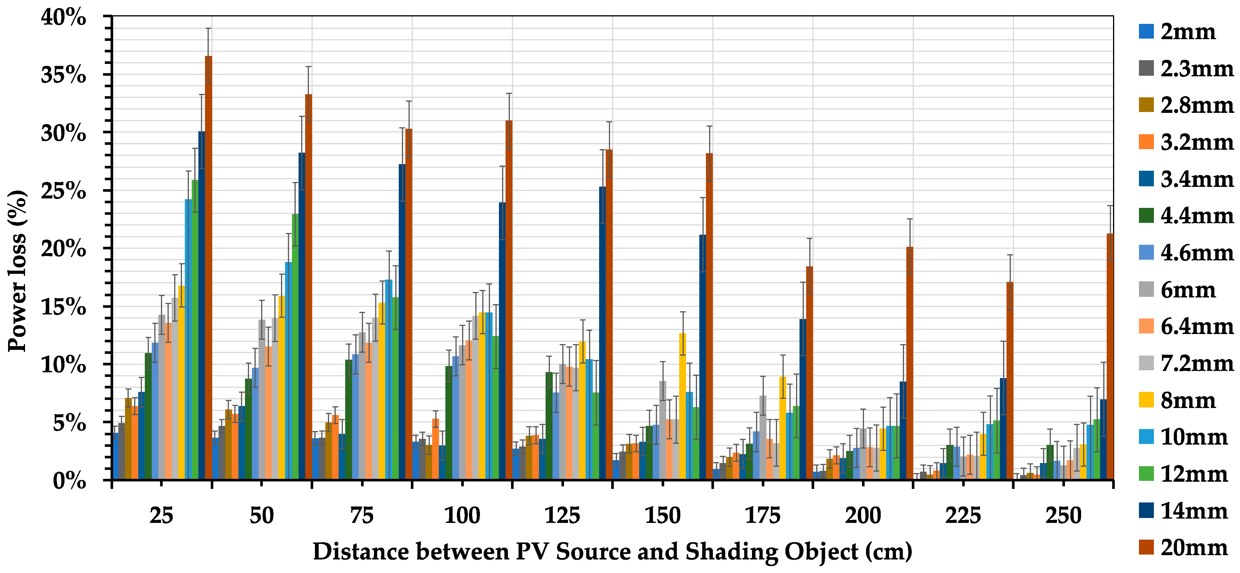
3.1.1. Analyzing the Factor of Distance
Figure 8 depicts the relationship of the percentage of power loss with the distance between the thin shading object and the PV module. The first noteworthy observation is the distinction of how shading objects at a 25 cm distance clearly induce significantly more power loss as compared to scenarios in which the objects are positioned at 250 cm from the PV module. The effect of distance is notably pronounced with smaller-sized objects, as exemplified by the clear trend observed at 3.2 mm. At this dimension, the power loss markedly decreases from 6.39% at 25 cm to a statistically insignificant 0.44%, marking a reduction of more than 12 times across the distance range from 25 cm to 250 cm. Notably, for power loss exceeding 10% at 250 cm, the object thickness needs to surpass 14 mm, which emphasizes the significance of distance as a critical factor.
The visual observations align with statistical analyses, in which the correlation between distance and thickness yields p-values of less than 0.001 in a two-tailed statistical bivariate correlation analysis. To validate the observed trends, a statistical assessment of power loss with distance was conducted. The initial Komogorov–Smirnov normality test exhibited a p-value of less than 0.01, necessitating a log transformation to meet normality assumptions. Subsequent tests confirmed conformity to the normality assumptions. Utilizing a general linear model, the outdoor data confidently establishes the statistical significance of distance as a factor to power loss. However, this significance diminishes beyond a distance of 175 cm, reaching reduced but still notable levels up to 200 cm. Interestingly, at distances of 225 cm and 250 cm, no statistically significant values over power loss were observed. Therefore, from this experimentation, distance as a factor is statistically significant up to a distance of 200 cm from the PV module, beyond which its impact on power loss diminishes substantially when thin object shading affects a PV module.
3.1.2. Analyzing the Factor of Object Thickness
The statistical analysis reinforces the significance of the thickness variable in influencing power loss. Notably, within the range of thicknesses from 3.2 mm to 20 mm, the level of significance is consistently high, with p-values less than 0.01. As thickness decreases to 2.8 mm, the statistical significance remains present, with a p-value of 0.01. However, below 2.8 mm thickness, specifically at 2.3 mm and 2 mm, the thickness becomes statistically insignificant in relation to power loss. This leads to the conclusion that thickness is a significant factor for object thicknesses of 2.8 mm and larger. The increasing significance with thicker objects aligns with expectations as a greater shaded area is present, intensifying the impact on power loss. This investigation extends to pinpointing the threshold at which the shadow effect becomes negligible, considering both distance and thickness as critical variables. The statistical analyses conducted reveal that the shading impact of thin objects, with a thickness of less than 2.3 mm coupled with distances beyond 225 cm, is statistically insignificant, resulting in a 1.65% power loss. This implies that beyond this specific combination of minimal thickness and considerable distance, the shadow’s influence on power loss diminishes to the point of becoming statistically insignificant.
3.2. Laboratory Experimentation Analysis Using the Solar Simulator
The visual analysis using the solar simulator shown in
Figure 9 shows a relatively linear increase in power loss as object thickness increases from 10 cm to 40 cm. This trend emphasizes the direct and predictable impact of thickness on power loss under these controlled conditions. In contrast, the examination of total shadow yields a distinctive pattern as the distance increases. The moving average trend lines shown in red indicate that the total shadow percentage undergoes a notable and pronounced increase, particularly within the range of 2 mm to 10 mm, as distance increases. A closer look into the formation of shadows, specifically distinguishing between the umbra and penumbra, reveals a crucial dynamic. At distances of 10 cm and 20 cm, the percentage of the penumbra closely mirrors the percentage of power loss, suggesting a strong correlation. However, at 30 cm and 40 cm, a drastic decrease in the umbra is evident, especially with thinner objects, signifying a rapid increase in the penumbra. This observation highlights the distinctive and prominent nature of the penumbra, even at a relatively short distance of 40 cm from the PV cell. Consequently, the increased formation of the penumbra emerges as a key factor contributing to the overall rise in total shadow as distance increases.
The investigation delves into the relationship between total shadow and power loss, shedding light on the crucial factors influencing the efficiency of PV modules in the presence of thin object shading. The Pearson correlation analysis reveals a highly significant correlation between the total percentage of shadow and power loss with a p-value of less than 0.001. This proves the impact of the overall shadow percentage in determining the extent of power loss when subjected to shading by thin objects. Moving beyond the holistic shadow assessment, individual components such as the umbra and penumbra are assessed for their correlation with power loss. The correlation between power loss and umbra is notably high, as evidenced by a p-value below 0.01. This aligns with expectations, considering the umbra’s prominence and its inherent highest intensity shadow. Surprisingly, the correlation between power loss and the penumbra, though less substantial than with the umbra, is still significant, with a p-value of 0.02. This unexpected finding prompts further investigation into the characteristics of penumbra shadows, suggesting that image analysis may offer insights into the nature of this correlation. It should be noted that no significant correlation is found between the umbra and penumbra, emphasising their distinct roles in influencing power loss in the context of thin object shading on PV cells.
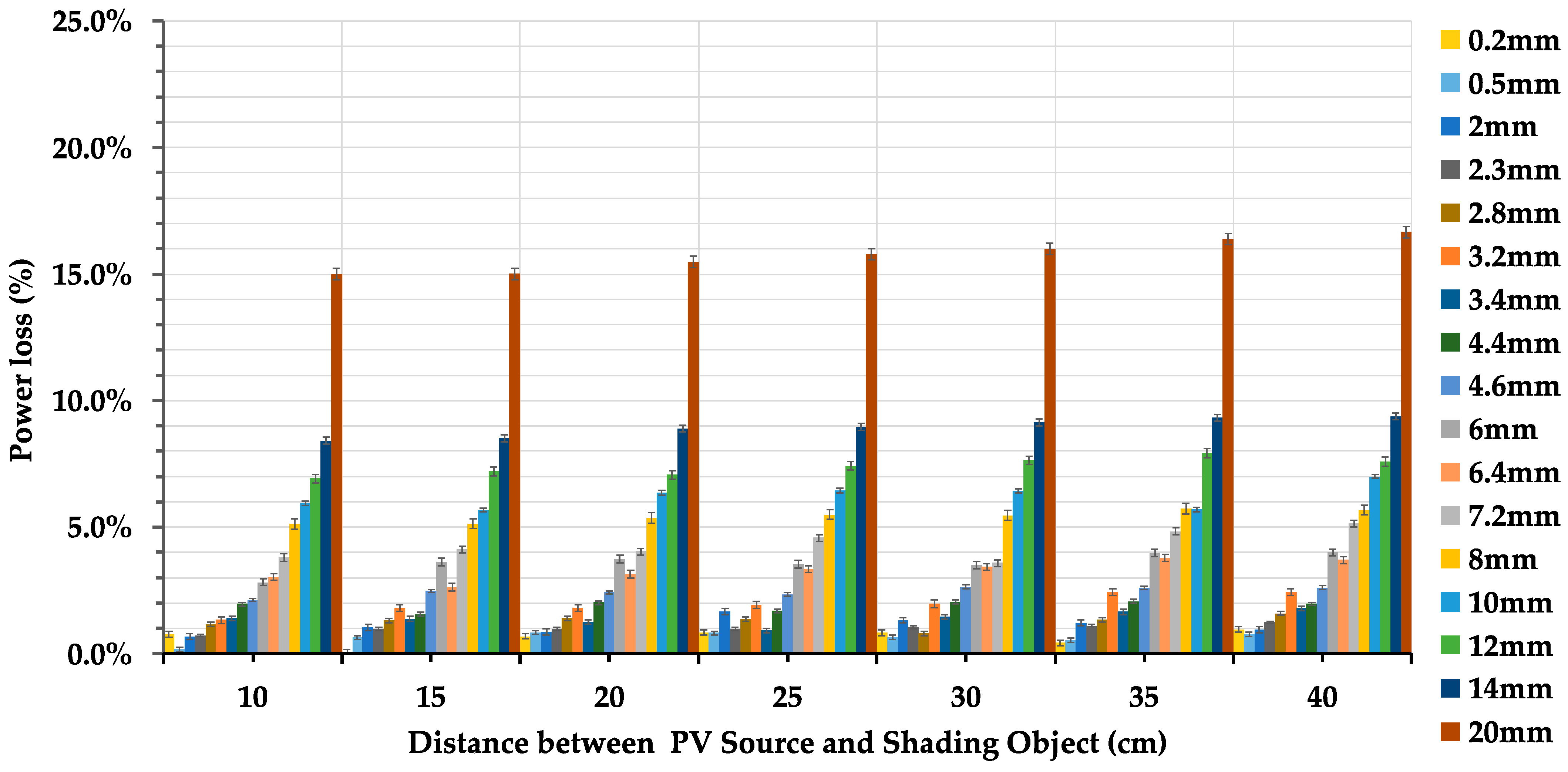
3.2.1. Analyzing the Factor of Object Thickness
Figure 10 reveals a noticeable exponential rise in percentage of power loss as the thickness of the thin object increases across all distances. To substantiate the significance of thickness as a variable, a comprehensive statistical analysis is essential. The power loss data violates the normality assumption, which is evident from its right-skewed distribution as indicated by both the Komogorov-Smirnov and Shapiro-Wilk normality tests, each yielding a
p-value of less than 0.01. To address this, a generalized linear model (GLM) is employed, utilizing the gamma distribution to account for the skewed nature of the data. The two-tailed
p-value derived from this model affirms the robust significance of the thickness variable as a determinant of power loss, with the
p-value being close to zero. This implies that, even in the controlled environment of laboratory experimentation, the thickness variable retains high statistical significance, emphasizing its crucial role in influencing power loss in the context of thin object shading on PV modules.
3.2.2. Analyzing the Factor of Distance
It is clearly shown that the change in power loss between a distance of 10 cm and 40 cm is not substantial. To consolidate this observation statistically, the same model used for analyzing thickness is applied. The results highlight a crucial finding: distance, as a factor in laboratory experimentation, is not statistically significant, as evidenced by a p-value of 0.144. This implies that, overall, variations in distance within the tested range (10 cm to 40 cm) do not exert a significant impact on power loss. It is important to note that the limitation of the solar simulator confined the investigation to a maximum distance of 40 cm. Interestingly, the trend observations, while indicating non-significance statistically, suggest that as distance increases, a subtle power loss also tends to increase. This observation contrasts with the trend observed in the outdoor experimentation, where an increase in distance results in a decrease in power loss. This discrepancy implies that there are other factors beyond distance, thickness, and object type that play a role in determining power loss in laboratory settings, emphasizing the complexity of the interactions influencing PV module performance in a laboratory environment. Furthermore, it is essential to acknowledge that the experimental limitations imposed by the equipment also result in a distinction between the range of distances examined in the indoor and outdoor experiments.
4. Comparative Discussion
While a direct comparison of power loss between outdoor and indoor experimentation was not feasible due to the distinct nature of the PV sources employed in each setting, the comparative analysis focused on the consistent formation of shadows on a uniform white surface. Utilizing the same white piece of paper in both scenarios allowed for a meaningful examination of shadow characteristics, forming the basis for the comparative discussion and enabling a focused analysis of shadow behavior as a key element in our comparative assessment. This aspect is being addressed to offer the readers visual representation of what is happening as distance increases gradually using both the solar simulator and outdoor experimentation, which is an additional step other researchers have neglected to showcase to readers. Throughout the outdoor and indoor experimentation methods, comprehensive photographic documentation was undertaken for all shadow combinations cast on the PV sources. These images facilitated side-by-side analyses to discern disparities in shadow formation with the aim of determining the direct comparability of laboratory and outdoor data.
Notably, from the comparative illustrations presented in
Figure 11, a significant observation pertains to the differences in background color, even with the use of the same white cardboard placed behind the thin object shadow. This observation can be attributed to the discrepancy in reflective light on the white plane, where outdoor settings reflect a greater amount of light and thus account for diffused lighting as opposed to a laboratory setting. In terms of shadow formation, distinct differences were evident. While outdoor shadows displayed a smooth transition between the umbra and penumbra, laboratory photos exhibited a distributed and uneven transition toward the penumbra. Furthermore, in all four illustrating instances of shade transposed from an exemplary 3.2 mm thin object as visualized in
Figure 11, a notable trend emerged indicating that the transition from umbra to penumbra shadows occurs more rapidly in a laboratory environment compared to the outdoor setting. Similarly, under the solar simulator, the reduction of shadow intensity diminishes more rapidly as the distance between the thin object and the PV cell increases. This consistent pattern across different object thicknesses and distances emphasizes the disparities in shadow behavior between laboratory and outdoor conditions.
In essence, due to significant differences in shadow transposition and thin object shading properties, direct comparison between laboratory and outdoor methodologies proved challenging. Despite this, a more in-depth analysis of shadow formation and quantifiable measures of such shadows may illuminate the variations between indoor and outdoor experiments. Moreover, the key takeaway is the awareness among researchers regarding these substantial principal discrepancies. Although laboratory experimentation provides accurate comparative results, the principles of shadow formation must be considered to avoid potential research misinterpretations. Nevertheless, the overall trends observed mainly during outdoor experimentation closely parallel those of [
16]: a substantial power loss occurs when a pole is positioned closer to the PV source, decreasing significantly as the pole moves farther away. Additionally, while seldom addressed in the literature, ref. [
16] notes that overhead wires often cast broad penumbra shadows on PV arrays instead of umbra. Building upon this conclusion, our study quantifies umbra and penumbra at all distance and thickness combinations, providing insight into the transition from umbra to the broader penumbra, leading to a notable decrease in power loss. However, even when broad penumbra is observed, the power loss may still exceed the significance level; for instance, objects thicker than 10 mm at 250 cm exhibit a power loss of more than 5%.


