Article

A Generalized Empirical Model for Velocity Deficit and Turbulent Intensity in Tidal Turbine Wake Accounting for the Effect of Rotor-Diameter-to-Depth Ratio

by
Kabir Bashir Shariff
and
Sylvain S. Guillou
*
Ecole d’Ingénieurs (ESIX Normandie), Université de Caen Normandie, UNICAEN, LUSAC, UR 4253, 60 rue Max Pol Fouchet, 50130 Cherbourg-Octeville, France
*
Author to whom correspondence should be addressed.
Submission received: 26 February 2024 / Revised: 21 April 2024 / Accepted: 23 April 2024 / Published: 26 April 2024
(This article belongs to the Topic Marine Renewable Energy, 2nd Volume)

Abstract

:
Commercial scale tidal stream turbines (TST) are expected to be deployed in shallow water where the depth varies from 1.5 to 3 turbine diameters. In this study, numerical simulation is conducted at realistic hydrodynamic conditions of potential tidal sites using the stationary actuator disc method at ambient turbulence varying from 5% to 20%, a range of rotor realistic rotor thrust coefficient from 0.64 to 0.98 and a rotor-diameter-to-depth ratio of 20% to 60%. The result shows that the TST wake is affected by the rotor-diameter-to-depth ratio, ambient turbulence, and thrust coefficient. The new empirical model is in accordance with the numerical simulation of a full-scale turbine and is validated with the TST experiment at different rotor-diameter-to-depth ratios with reasonable results in the far wake. This low computational model can benefit the investigation of tidal turbine parks at different configurations where the far wake is pertinent.

1. Introduction

Tidal currents are caused by the gravitational forces of the sun and the moon and are particularly concentrated in narrow straits. With an estimation of 800–1200 TWh [1], tidal energy will contribute to the much anticipated green energy transition. The mean hydrodynamic conditions of potential sites in Table 1 fall within sub-class B and C of the marine energy classification system [2]. As the energetic tidal sites are limited by size, depth, and shipping routes, the task remains to obtain the best approach to exploit this renewable energy. Several technologies have been proposed to harness tidal energy but the most promising technology so far is the tidal stream turbine (TST). The first-generation TSTs are usually sited in shallow water (predominantly below 50 m) where the depth varies from 1.5 and 3 turbine diameter [3].
Over the last decade, the tidal energy industry has recorded successful deployment and testing of full-scale TST at dedicated test sites and commercial project locations [17,18]. Commercial-scale tidal energy production requires a cluster network of TST in energetic sites. Recently, the Normandie Région in France has consented to the development of two pilot farm projects in the Alderney Race; the 11 MW Normandie Hydrolienne and the 17.5 MW Flowatt project [19]. A cluster network of turbine arrays can reduce costs by sharing infrastructure and collective maintenance. However, turbine interaction in the park affects the turbine performance in the form of the wake [20]. A wake can be simply defined as a zone perturbed flow behind the turbine. The two predominant wake features are the velocity deficit and the increased turbulence. The velocity deficit significantly reduces the available power for the turbine downstream while the increased turbulence induces fatigue load on the downstream turbine. The poor understanding of TST in realistic conditions has resulted in system failures after deployment causing reluctance on the part of investors due to the perceived risk of device failure [21]. This limited availability of full-scale turbine data remains among the challenges of the promising tidal energy industry, which inevitably leads researchers to resort to flume experiments and CFD simulations to investigate the hydrodynamics of tidal turbines.
Experimental studies using both porous discs [22] and the tidal turbine were conducted to investigate the turbine performance [23] and the wake effect in single and multiple turbine layouts. The experimental study [24] found the wake shape, length, and strength are significantly affected by the ambient turbulence but slightly affect the performance parameters. Reference [25] also found the ambient turbulence and the integral length scale affects the drag coefficient of the rotor. However, [26] suggests that though ambient turbulence significantly affects the wake, the turbulence length scale is insignificant. Chen et al. [27] studied the effects of rotor-diameter-to-depth ratios. The results show the increased rotor-diameter-to-depth ratio is comparable to an increase in thrust coefficient. Also, [28] investigate the hydrodynamics of wake at three different rotor-diameter-to-depth ratio. The results show the shear layer at a high rotor-diameter-to-depth ratio is elliptical as reported by [23] as a result of the wake compression due to the limited channel depth.
Similarly, numerical models are used to investigate the performance of both reduced and full-scale tidal turbines. The geometric resolved model is the most accurate model that provides realistic turbine loading [29]; however, it is computationally expensive. The Actuator Line Model (ALM) is an extension of the Blade Element Model (BEM) that accounts for the non-uniform loading on the turbine blades and provides a good representation of both near and far wakes [30]. There also exists the Actuator Disk Model (ADM) that represents the turbine as a porous disc; this model neglects the turbulence generated at the blade’s tip but has a good representation in the far wake. The ADM is widely used in large farms due to its low computational cost [31]. In addition to isolated turbines, an investigation of wake interaction in the tidal park has been carried out by several authors [3,32,33].
Moreover, empirical models are developed based on self-similar profiles of the turbine wake using the conservation law of mass and momentum. Over the last decade, empirical models for tidal turbines were developed to estimate the velocity deficit of tidal turbine wake. These models are developed mainly by calibrating wind turbine models to account for either the ambient turbulence [34] and/or the thrust coefficient [35] but do not take into account the diameter-to-depth ratio. The analytical models of velocity deficit and turbulence intensity of wind turbines require calibration to have a reasonable estimation of turbine wake. Unlike wind turbines, first-generation tidal turbines are located in shallow water limited by the depth which affects wake development.
As already established in the literature, the wake behind a tidal turbine is influenced by at least three parameters; the flow condition, the turbine itself, and the site configuration. The objective of this study is to propose a low computation empirical model to estimate the velocity deficit and turbulence intensity in tidal turbine wake accounting for the variation in ambient turbulence, thrust coefficient and rotor-diameter-to-depth ratio. This should be used in conjunction with an optimization algorithm to find out the position of the turbines regarding the power afterwards. The study at different rotor-diameter-to-depth ratios is significant as the water depth varies with the tidal cycle. A first attempt to estimate the added turbulence in the wake of the full-scale tidal turbine is reported by the authors [36]. This paper is part of a project intended to develop a generic model to optimize electricity production in a tidal turbine park.
The rest of the paper is organized as follows. Section 2 describes the existing analytical model for wind and tidal turbine applications. Section 3 presents the methodology to set up the numerical model using the actuator disk method and the development of the empirical model. The result of the developed empirical model for the velocity deficit and turbulence model is developed and validated with experimental data in Section 4. Lastly, the discussion and conclusion are presented in Section 5 and Section 6, respectively.

2. Analytical Modelling

2.1. Velocity Deficit Models

The far wake behind a disc is approximately Gaussian with the minimum velocity at the turbine core [37]. The wake velocity behind a turbine is a product of a stream function and a shape function. The velocity deficit in the wake of the turbine is expressed as Equation (1):
Δ U U = U U w U
where U is the upstream velocity and U w is the wake velocity. The classical models for velocity deficit in the wake of wind and tidal turbines are briefly discussed below.

2.1.1. Jensen Model

The analytical model of velocity deficit of wind turbines developed by Jensen [38] and modified by Katic et al. [39] is based on momentum balance behind the turbine. The velocity deficit is uniformly distributed using the top-hat shape function and assumes a linear wake expansion. This model neglects the near wake and is extensively used in wind farm commercial codes like WAsP, WindSim, and WindPRO. The Jensen velocity deficit is expressed as Equation (2):
Δ U U = 1 1 C T 1 + α x r 0 2
where r 0 is the turbine radius, C T is the thrust coefficient, x is the downstream distance, and  α is the rate of wake expansion coefficient. Suggested values for α are 0.075 for onshore and 0.05 for off-shore turbines [40].

2.1.2. Bastankhah and Porté–Agel Model

The Bastankhah–Porté Agel (BP) model [41] of velocity deficit is based on the mass and momentum conservation equation. The model uses a Gaussian shape function and assumes also a linear expansion of wind turbine wake downstream. The velocity deficit model is expressed as Equation (3):
Δ U U = 1 1 C T 8 k * x / d 0 + 0.2 β 2 × exp 1 2 k * x / d 0 + 0.2 β 2 z z h d 0 2 + y d 0 2
y and z are spanwise and vertical coordinates, respectively. k * and β are empirical constants depending on the turbulent intensity and thrust coefficient, respectively.

2.1.3. Lam and Chen Model

This is potentially the first analytical model developed for the tidal turbine application. The model is developed from the wake distribution of a propeller ship with a Gaussian distribution. The velocity deficit of Lam and Chen’s model [42] is expressed as Equation (4):
Δ U U = ( U U min ) U × exp r w + 0.081 x + r 0 2 2 0.081 x 2

2.1.4. Lo Brutto Model

Lo Brutto et al. [34] express the wake of a tidal turbine as a function of turbulent intensity and thrust coefficient. The proposed model is based on exponential wake expansion and a top-hat shape function developed by Jensen [38]. The model is used to simulate a small tidal park at different turbulent intensities but is limited to a low rotor-diameter-to-depth ratio (20%). The wake expansion according to exponential law depends on ambient turbulent intensity. The velocity deficit is expressed as Equation (5):
Δ U U = 1 1 C T r w r 0 2 r w = c ( I 0 ) [ 5.58 ( 1 e 0.051 x D ) + 1.2 ] c ( I 0 ) = 15.542 I 0 2 + 21.361 I 0 + 0.2184
where r w is the wake radius, r 0 is the rotor radius, x / D is the normalized distance downstream, c ( I 0 ) is a quadratic function of the ambient turbulence.
Other authors [35,43,44] use the CFD results of the tidal turbines to calibrate the velocity deficit models of wind turbines. These calibrated models are extended for application in a simple tidal park [45,46]. Table 2 presents a summary of the existing velocity deficit models with the proposed model.

2.2. Turbulence Intensity Model

Turbulence intensity is defined by [51] as the ratio of the standard deviation of fluctuating velocity ( U rms ) to the mean speed ( U ¯ ) expressed as Equation (6):
I = U rms U ¯
The turbulent intensity in the wake of a turbine is the contribution of ambient turbulence in the flow and the added turbulence generated by the turbine expressed by [52] as Equation (7):
I w = I amb 2 + I + 2 0.5
where I w is the total turbulence in the wake, I amb is the ambient turbulence and I + is the added turbulence by the rotor. The added turbulence is the additional turbulent kinetic energy induced by the turbine and the shear layer developed at the tip of the blade. The empirical models were developed to estimate the added turbulence for wind turbine applications [49,53,54]. These models are outlined in the previous work of the authors [55].

3. Methodology

3.1. Numerical Method

Numerical simulation is performed with open-source code OpenFOAMwith the turbine represented as a porous disc using the actuator disc method (ADM). The ADM applies a uniform thrust force along the disc surface to replicate the pressure jump across the turbine during the energy extraction. Though the ADM underestimates the wake in the initial near wake, it provides acceptable results in the far wake region [56]. The ADM is widely used in wind and tidal farm applications [57]. The uniform thrust force is evaluated as Equation (8):
T = 1 2 ρ C T S U 2
where ρ is the fluid density, S is the rotor cross-sectional area, U is the upstream velocity and C T is the thrust coefficient. For multiple turbines, the use of the upstream velocity is debatable due to the wake effect. Therefore, the thrust force is evaluated with the local velocity at the disc location as Equation (9):
T = 1 2 ρ K S U d 2
where U d is the velocity at the disc and K is the resistance coefficient which relates to the thrust coefficient as C T = K 1 + 1 4 K 2 . The thrust force is added as a source term to the momentum equation and solved along with the continuity equation. A standard κ ϵ turbulence model is used for Reynold’s stress closure with a turbulence correction to compliment the turbine-generated turbulence as suggested by [58,59,60]. The κ ω SST turbulence model is shown to provide good results because of its ability to represent the near wall and free stream. Nevertheless, it is the same in the vicinity of an actuator disk with κ ϵ , as shown by [56], who studied different turbulence models for actuator disks. The results from the work of [56] indicated that the use of standard κ ϵ for an actuator disk is sufficient to provide a good representation of the wake without the use of turbulence source term. For this reason, subsequent studies on this project use the κ ϵ turbulence model.
The model is validated in the previous work of the authors [55].

Case Set-Up

A full-scale turbine is located 10 D (D is turbine diameter) from the inlet, the length of the domain is 50 D, the channel width is 20 D and four channel depths (H) are considered: 10 m, 25 m, 35 m, and  50 m, representing the tidal straits depth as shown in Table 1. In each case, the rotor is situated at the mid-depth of the channel. Three rotor-diameter-to-depth ratios (DH) were studied in a channel with realistic flow conditions. For simplicity, the three cases are labeled as DH20, DH40, and DH60 representing the diameter-to-depth ratios of 20%, 40%, and 60%, respectively. The rotor diameter corresponding to each channel configuration is presented in Table 3. The numerical domain has a low blockage ratio for all the configurations with 2.36% for the DH60. The blockage ratio is defined as the ratio of the actuator disc to the total cross-sectional area of the domain. A low blockage ratio does not affect the flow, and therefore, does not require a correction term [61]. Figure 1 shows the different diameter-to-depth ratios of the three configurations.
The numerical domain is discretized by structured grid cells with refinement close to the turbine. In the previous work of the authors [55], grid sensitivity was carried out at different mesh and cells per diameter (CPD). In total, 25 CPDs across the disc surface for the Δ y (transverse) and Δ z (depthwise) were chosen as the result independent from mesh. This mesh based on 25 CPDs is used for the different rotor diameters presented in Table 3. The CPDs along the Δ x (streamwise) direction representing the thickness of the disc are 4. The region far away from the disc is represented by a coarse mesh with a geometric growth rate of 1.2. This numerical model has been validated previously [55], with a three-bladed experiment by Mycek et al. [24].
The numerical model is based on a realistic hydrodynamic condition of the Alderney Race [4]. At the channel inlet, a logarithmic velocity, a constant turbulent kinetic energy (TKE), and dissipation are defined as expressed in Equation (10). Where the friction velocity U * = 0.1109  m/s, the mean inlet velocity U = 2.7 m/s is similar to the mean velocity in the Alderney Race [4]. In the study, the bottom roughness of the channel is not considered. Instead, we set a no-slip condition on the bottom wall, as well as a symmetry condition on the top and lateral walls. An outlet condition corresponding to atmospheric pressure is set on the domain.
U = U * κ ln z z 0 , k = 3 2 I 2 U 2 , ϵ = C μ 3 4 k 3 2 L
To propose a generic model, the ambient turbulent intensity ranging from 5% to 20% is considered, providing a global representation of turbulence at potential tidal sites (see Table 1). Similarly, a set of turbine thrust coefficients C T allowing application at different configurations is used as presented in Table 4. In the case of a full-scale tidal turbine, there are no experimental results available for adjusting the parameters for the turbulence source term to account for turbine effects; therefore, a standard κ ϵ is used instead. Empirical models, however, require a defined value of the turbulent intensity upstream of the turbine. Due to the turbulence dissipation downstream, especially at high turbulence intensity, this value may be uncertain at the turbine position in the simulation. Therefore, the upstream region is kept stable by maintaining the inlet turbulence condition. This means that a turbulence source region is set upstream from the inlet to the turbine location to maintain the same turbulence intensity and dissipation at the inlet. This will ensure a constant turbulence perceived by the rotor as the inlet condition neglecting the decay in channel flow. This is analogous to the turbulence source term used for wind turbines by El Kasmi and Masson [58].

3.2. Empirical Method

The proposed model is derived using the numerical results as the reference data using a curve fitting tool in Matlab. The empirical parameters are derived from a nonlinear least square solver lsqnonlin in Matlab. For instance, to obtain the empirical model for the added turbulence, the numerical data at different ambient turbulences, thrust coefficients and rotor-diameter-to-depth ratios are combined in a single matrix with the first and second column representing the downstream distance X and numerical added turbulence, respectively. For each data set, a corresponding value of ambient turbulence, thrust coefficient and rotor-diameter-to-depth ratio is set as defined in the numerical setup in columns three, four and five, respectively. An objective function defined in curve fitting is used in the lsqnonlin optimization. The non linear least square optimization in Matlab is expressed as Equation (11).
min x | | f ( x ) | | 2 2 = min x ( f ( x ) 2 )
where f ( x ) is expressed as power law in Equation (13) subjected to constraints defined by Equation (12) as:
0.05 I o 0.2 0.64 C T 0.98 0.2 D H 0.6

4. Results

4.1. Added Turbulent Intensity Model

Turbulence intensity in the wake is the square sum of ambient and added turbulence expressed in Equation (7). Added turbulent intensity is the contribution of the shear and turbine-generated turbulence. The ambient turbulence, shown in Figure 2, is the turbulence close to the lateral wall and stable in the flow; therefore, it is sufficient to propose a model for added turbulence to estimate the turbulence in the wake of the tidal turbine. However, in numerical simulation, there is a continuous decay in turbulence in channel flow in the absence of turbulence source term. Consequently, the turbulence along the lateral wall with decay is used as ambient turbulence to ensure good comparison between the numerical and empirical model. In a previous study by the authors [55], the centreline added turbulence intensity of a single turbine for a 20 m diameter at the best theoretical thrust coefficient (Betz limit) is developed using curve fitting in Matlab. The approach is generalized to accommodate a range of rotor thrust coefficients, DH ratios, and different ambient turbulent intensities. The generalized added turbulence model is expressed as Equation (13):
I + = a X X 0 D b × exp y 0 y 2 + z 0 z 2 r w 2 a = 0.407 D H C T 4.83 + 0.179 , b = 0.681 I eff + 0.472
where a and b are the functions depending on D H , C T and the I eff . I eff is the effective turbulence intensity which is the root-square sum of the added turbulence and the local ambient turbulence I amb with decay along the lateral wall in a single turbine. The turbulence intensity in the wake is reconstructed using Equation (7) and compared with the tidal turbine experiment of Mycek et al. [24] at DH35 and Stallard et al. [3] at DH60. Figure 3 shows the model provides reasonable results in comparison to the experimental data, especially in the far wake region. It is noted that the model does not provide good approximation in the near wake region (i.e., X / D < 5 ). However, in the far wake, (i.e., X / D > 5 ), the turbulence intensity obtained with the proposed model has a good fit with the experimental data. In our study, there is a limitation in the near wake region as the actuator disk underestimates the near wake region as reported by Lo Brutto et al. [34]. In a turbine array, the turbines are usually positioned in the far wake region where the wake recovery is high to achieve more power and reduce fatigue loading. Therefore, the low accuracy of the model in the near wake is not consequential.

4.2. Velocity Deficit Model

The velocity deficit is the sum of the stream function and the shape function. To estimate the centerline wake velocity of the tidal turbine, the wake radius model is substituted in the Jensen model presented in Equation (2). The top-hat shape profile of the Jensen model estimates the average velocity in the wake, while the numerical data provide the minimum wake velocity in the form of a Gaussian profile, as shown in the Appendix A. Assuming the velocity deficit in a lateral plane is Gaussian shape, Lo Brutto et al. [34] proposed a relation for maximum velocity deficit for the Jensen model as Equation (14):
Δ U def , max = Δ U def , aver r w σ 2
where σ = r w / 2.59 is the standard deviation. The maximum velocity deficit Δ U def , max , henceforth Δ U def , can now be compared with the minimum velocity along the centreline in numerical data. In the present model, we propose directly using a Gaussian model and then directly estimating the velocity deficit in the wake without using a correction coefficient. The velocity deficit is then expressed as Equation (15):
Δ U U = 1 1 C T r w r 0 2 × exp y 0 y 2 + z 0 z ) 2 r w 2
where C T is the thrust coefficient, r w is the wake radius downstream and r 0 is the rotor radius. The exponential function provides the Gaussian shape profile along the lateral plane. The proposed velocity deficit model is compared with the tidal turbine experiment of Stallard et al. [3] and Mycek et al. [24] as shown in Figure 4. The model is in good agreement with experimental data in the far wake region ( X / D > 5 ), which is the objective of this study. However, the model is less accurate in the near wake due to the underestimation of the wake using a stationary ADM. High-fidelity numerical results are necessary to obtain accurate results in the near wake. This is computationally expensive for a large data set to propose a generic model.

Velocity Deficit Wake Radius

The classical theory of turbulence shows the far wake behind a disc is axisymmetric and self-similar in a free shear flow. However, in a tidal stream, the wake is also regarded as self-similar but transmutes from axisymmetric to 2D Gaussian due to the depth constraint [62]. Figure 5 shows the variation in the wake profile along the centerline (i.e., mid-surface MS) and the free surface FS at different rotor-diameter-to-depth ratios at 3 D downstream. At a low diameter-to-depth ratio (i.e., DH20), the normalized lateral wake profile is Gaussian along the centerline (MS); however, the wake effect is insignificant along the free surface. This indicates the wake is axisymmetric at 3 D downstream at a low diameter-to-depth ratio. As the DH ratio increases (i.e., Figure 5, DH40 and DH60), the wake along the free surface (FS) begins to develop into a 2D Gaussian profile. In addition, ref. [34] reported that an increase in ambient turbulence intensity also increases the transition from axisymmetric to a 2D Gaussian profile at a given rotor diameter to depth ratio.
The wake radius is estimated at 3 σ using the full-width half maximum approach reported by the authors [55] (see Appendix A). The velocity deficit radius expands higher at DH20 because the expands in all directions to a great distance downstream before reaching the channel depth limit. As the DH increases the wake expansion is limited in the vertical plane creating an elliptical wake due to the wake compression, as shown in Figure 6a. The turbine wake expansion is reported to increase with turbulence intensity [34,55] due to enhanced mixing but is insensitive to the thrust coefficient as shown in Figure 6b. The empirical wake radius based on power law is expressed as Equation (16):
r w = c X X 0 D d
c = 2.15 D H 0.283 , d = 0.29 for   I eff < 8 % ; c = 2.36 + 1.834 I eff D / H , d = 0.27 D H 0.275 for   10 % I eff < 20 %
where c and d are functions depending on the DH, C T and I eff , respectively. The difference in the parameters c and d at low and high turbulence might be due to the difference in wake structure. The wake expansion is less at low ambient flow resulting in the largely axisymmetric wake while at high turbulence intensity, the wake expands faster to reach the vertical boundaries modifying the structure to a 2D Gaussian wake.
The wake radius model comprising the DH ratio and ambient turbulence provides good results in comparison to the numerical data as shown in Figure 6. In Figure 6a, the increase in a trade-off exists between an increased wake radius at high turbulence and a decreased wake radius at a high DH ratio. The increase in wake expansion at high turbulence is due to enhanced mixing and diffusion while the decrease at high DH is due to the limited channel depth.

5. Discussions

5.1. Effect of the Channel Depth

Four different channel depths of the potential commercial tidal site are studied under the same hydrodynamic conditions. Figure 7 shows the center-line velocity deficit and turbulence intensity for different channel depths. Irrespective of the diameter or the channel depth under consideration given in Table 3, the hydrodynamics of the flow is the same for a given diameter-to-depth ratio. For each case studied, the boundary condition and the model setup are identical. As the tidal turbine is bounded by limited depth, the notable parameter should be emphasized and considered in the hydrodynamics of the flow. Thus, to propose a generic model, a particular channel depth with a different rotor-diameter-to-depth ratio is sufficient to provide a generic representation of the channel size. The variation in DH ratio (dimensionless) provides different wake scenarios in the domain to develop a generic model. The wake expansion along the lateral plane is presented for several diameter-to-depth ration Figure 8.

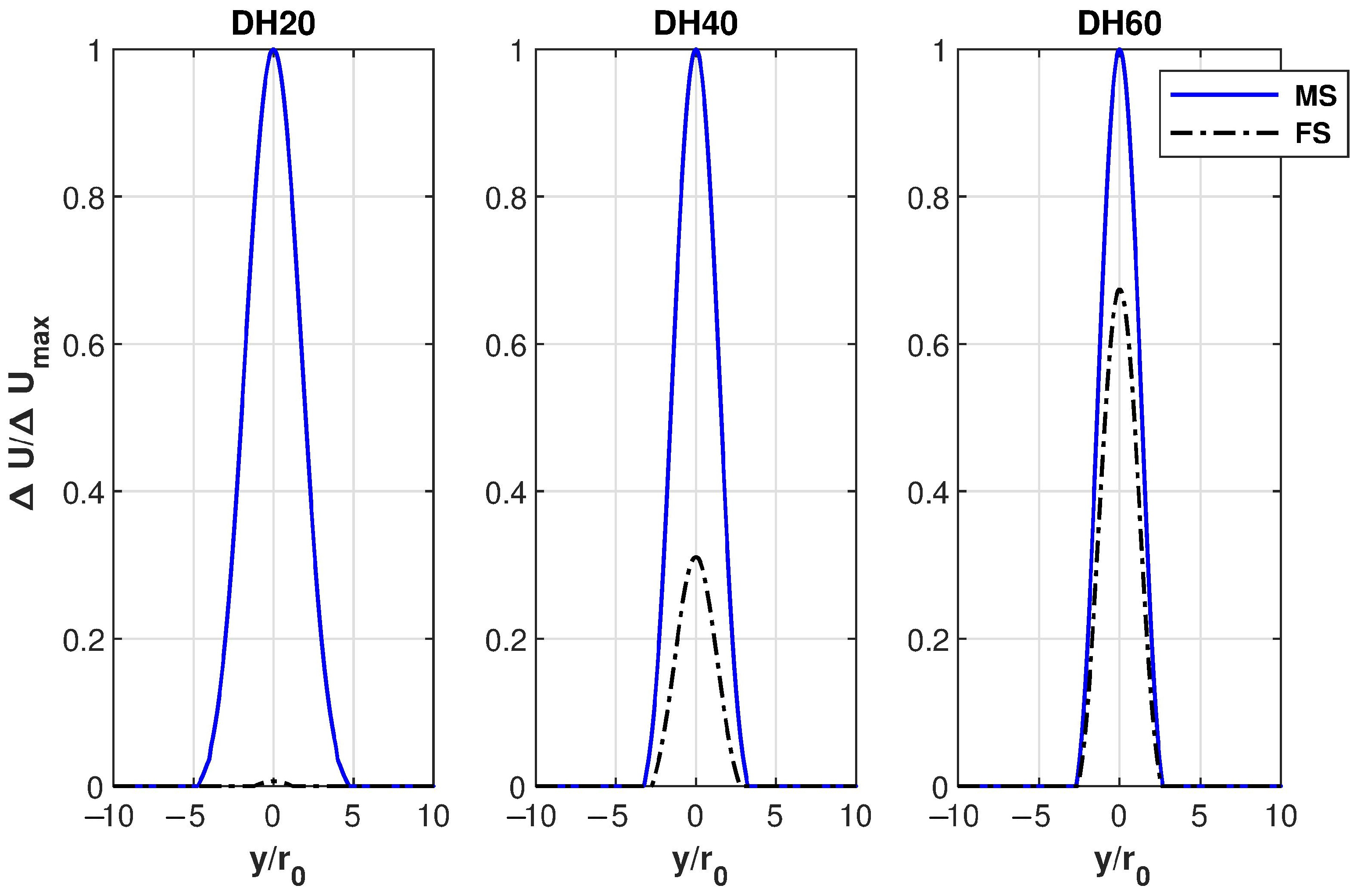
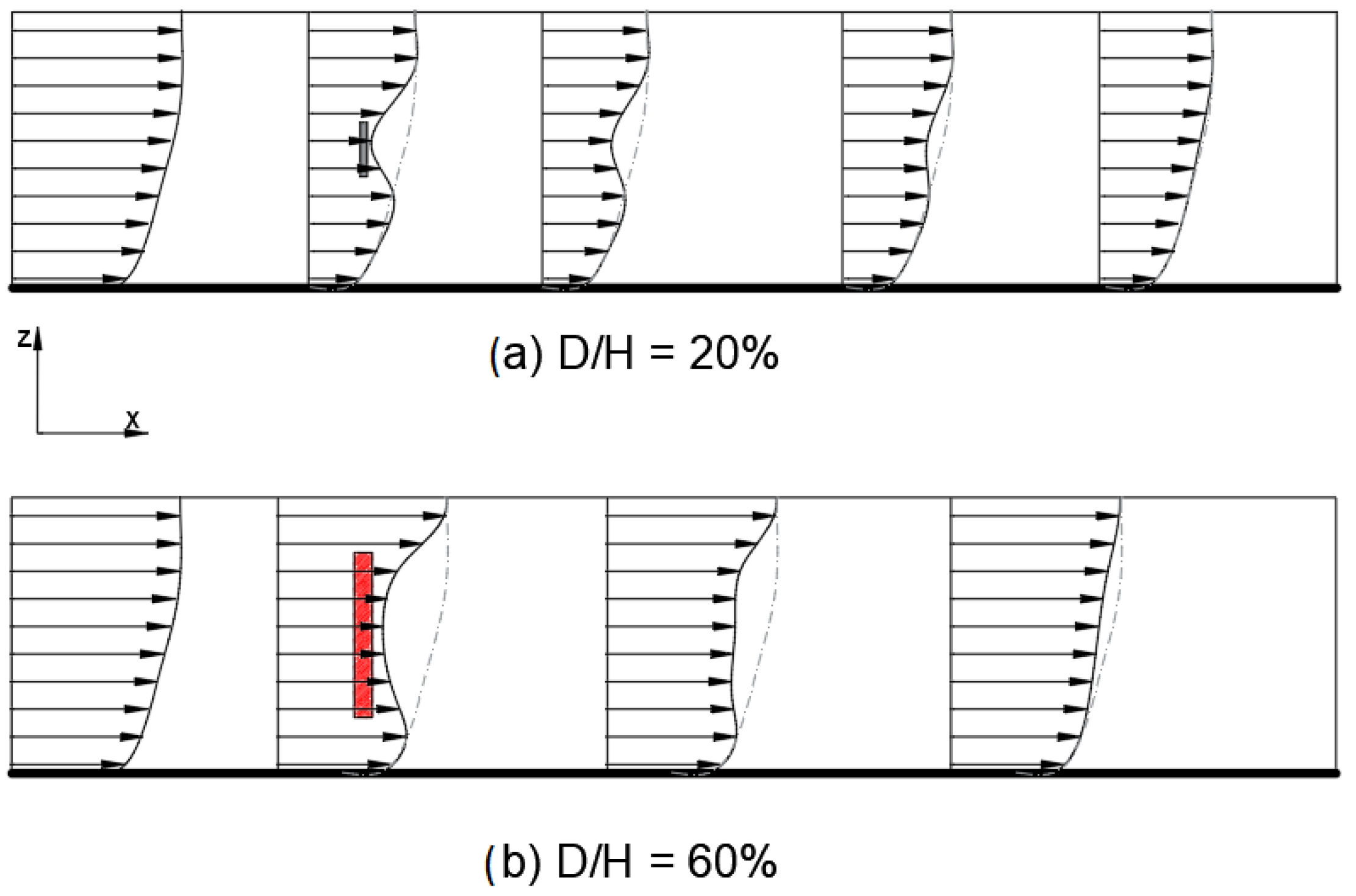
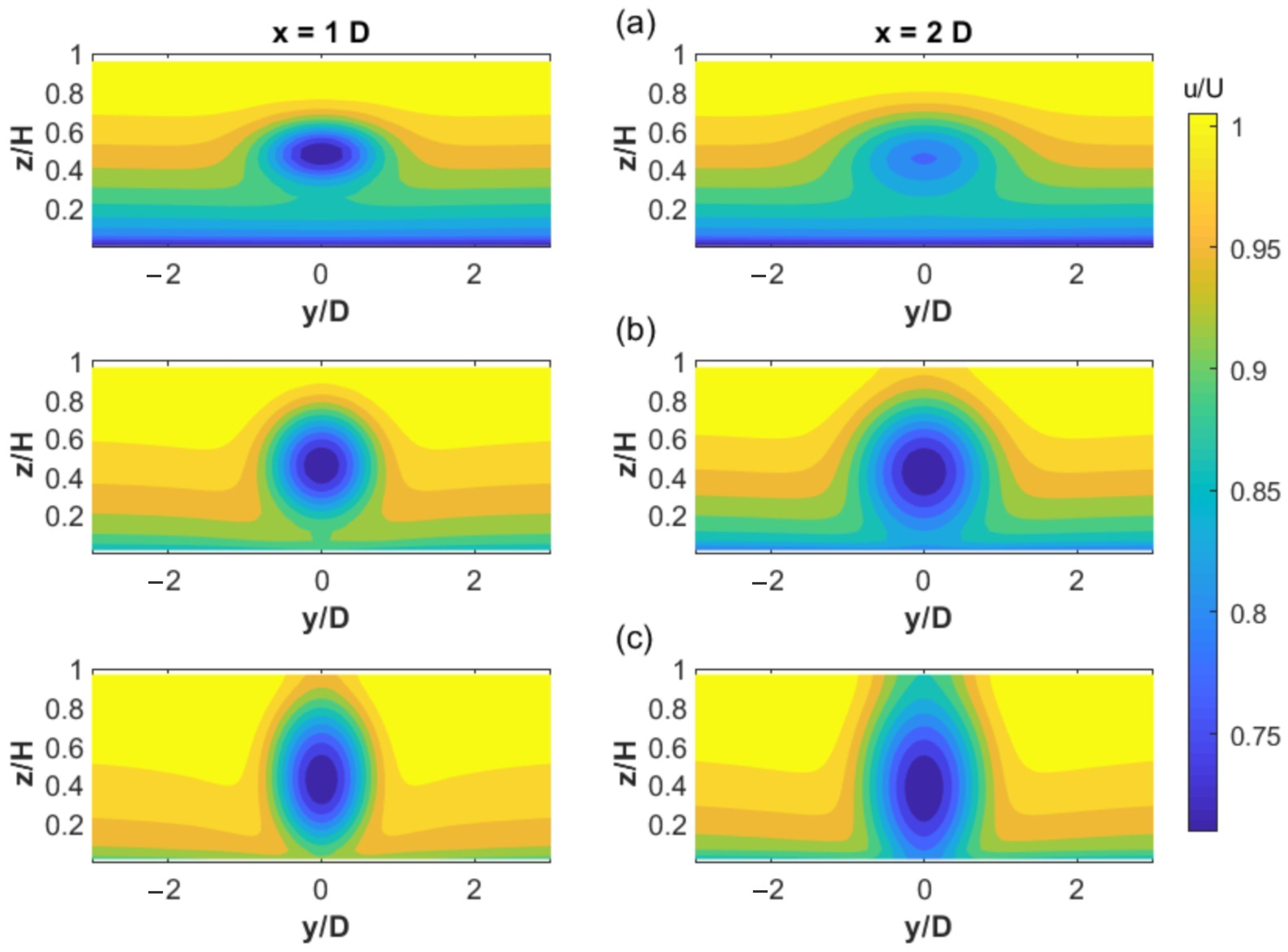
5.2. Effect of the Rotor Diameter to Depth (DH) Ratio

The DH ratio is the area the rotor covers along the vertical plane. The rotor wake recovery is affected by the bypass flow. Bypass flow is a region around the turbine with ambient flow conditions. The momentum exchange by the rotor reduces the velocity of flow creating a wake that propagates downstream. At a low rotor-diameter-to-depth ratio (i.e., DH20), the wake recovery process is faster as the flow in the bypass region is sufficient to cause mixing between the low velocity at the rotor’s core and the ambient flow in the bypass region. However, at a high DH ratio (i.e., DH60), the velocity deficit along the rotor is substantial compared to the free stream flow in the bypass region, therefore lagging the wake recovery to the upstream condition. The lower bypass flow region is associated with high turbulence and low velocity (bottom wall effect) while the upper bypass flow region has higher velocity and low turbulence effect (free surface effect). This causes the drift of the wake upward in a high rotor-diameter-to-depth ratio as shown in Figure 9. Experimental studies reported the drifting of vertical profile [27] and the DH ratio is interpreted as an increase in the thrust coefficient.
The mean shear layer exists at the interface of the low velocity at the rotor core and high ambient flow (by-pass flow region). The mean shear expands from the rotor tip until finally reaches the center line. The shear layer expansion occurs in the transverse and vertical direction at a low rotor-diameter-to-depth ratio. However, an experimental investigation of the high rotor-diameter-to-depth ratio (DH60) by Stallard et al. [23] shows about 1.5 times the expansion rate higher in the transverse direction than in the vertical plane due to the limited channel depth. A similar compression of the radius and shear layer thickness has also been reported in similar studies by Zhang et al. [28], forming a slightly elliptical profile by virtue of proximity to vertical boundaries. Figure 10 supports experimental studies that show an incomplete vertical development of wake at rotor-diameter-to-depth ratio due to the limited channel depth.
As for all bluff bodies in a flow, the presence of the turbine generates a wake that propagates behind the turbine. The wake of the turbine in free shear flow is approximately axisymmetric [37]. However, in shallow water depths, the structure of the wake can be affected by the limited depth. Olczak et al. [62] show the wake transmute from axisymmetric to transverse Gaussian profile. The transition to the 2D Gaussian profile is accelerated by the rotor-diameter-to-depth ratio as shown in Figure 5. The normalized lateral profile close to the free surfaces becomes Gaussian similar to the centerline profile as the rotor diameter to depth increases. The wake transit from axisymmetric to 2D Gaussian due to the limited depth at DH60. The wake expansion along the lateral plane is limited at a high DH ratio as shown in Figure 8.
In addition, the effect of DH at C T = 0.89 and 10% turbulence intensity is presented in Figure 11. The normalized velocity is substantially affected by the DH ratio due to the wake expansion but the turbulent intensity variation at different DH ratios is minimal. The flow recovery at high DH is lessened due to the weak mixing between the low-velocity flow at the rotor core and the high-velocity bypass flow.

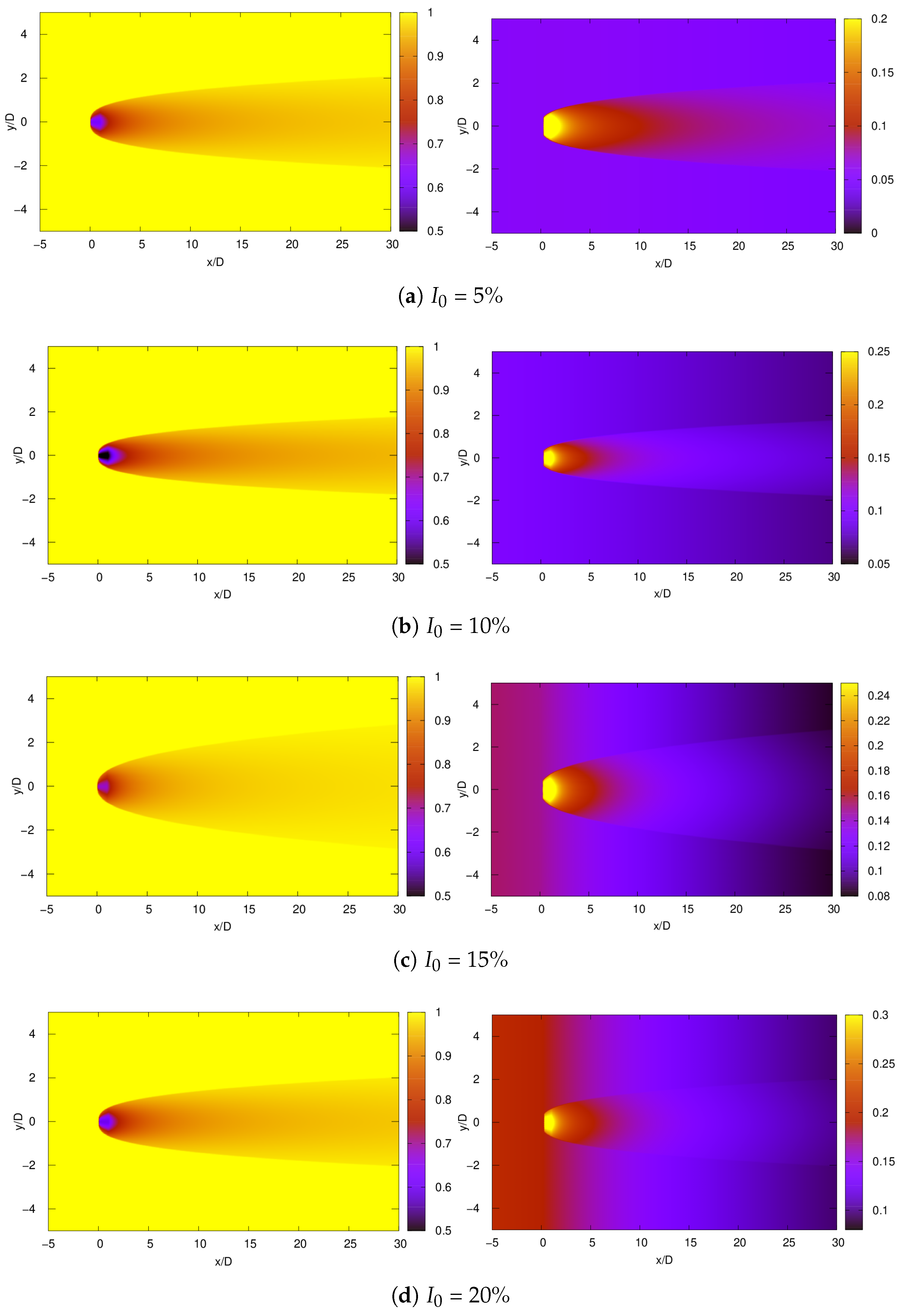
5.3. Effect of Ambient Turbulence

Figure 12 presents the normalized velocity and turbulent intensity at DH40 and C T of 0.89. The velocity deficit and turbulence intensity recovery are faster at high ambient turbulence. The turbulence in the wake recovers at 15 D and 9 D for 10% and 15% inflow turbulence, respectively. Other experimental [24,25,63] and numerical [64] studies of the wake effect illustrate the reduction in velocity deficit and quick flow recovery at high turbulent flow. The proposed model provides reasonable results compared to the numerical data, especially in the far wake region.
The wake of turbulent intensity recovers at 5 D when the ambient turbulence is 20%. For 15% ambient turbulence, the wake recovery is achieved around 10 D downstream and 15 D for 10% ambient turbulence. At low ambient turbulence, the centerline turbulent intensity does not fully recover due to slow mixing and diffusion of the wake. The contour of normalized velocity and turbulent intensity is presented in Figure 13.

5.4. Effect of Thrust Coefficient

Similarly, the effect of the thrust coefficient at 10% ambient turbulence is shown in Figure 14. An increase in C T can also be interpreted as increasing the drag force that causes the momentum exchange across the disc. High C T creates a large velocity deficit close to the rotor producing high turbulence in the near wake. The increased thrust coefficient is largely effective in the near wake region. This variation due to the thrust coefficient is well represented by the proposed model in the near wake. However, far away from the rotor, the effect of C T is less significant as the flow is largely homogeneous, thus reaching the recovery state.

6. Conclusions

The objective of this study is to develop a general empirical model to estimate the far wake behind a tidal turbine. Numerical simulations were conducted at realistic hydrodynamic conditions and channel configurations. From the numerical results obtained, we conclude that:
  • The ADM underestimates the velocity deficit and turbulence intensity in the near wake; howver, it provides acceptable results in the far wake.
  • For a given DH ratio, the center-line velocity deficit and turbulence intensity are identical irrespective of the turbine diameter.
  • The bottom and surface effect can affect the wake when the rotor-diameter-to-depth ratio is high.
In general, the following conclusions are obtained:
4.
The TST wake is not affected by the channel depth but rather by the rotor-diameter-to-depth ratio.
5.
The DH ratio affects the wake expansion due to the limited depth in shallow water causing compression in the mean shear layer in the vertical direction
6.
Increasing ambient turbulence facilitates wake recovery due to the enhanced mixing process.
7.
A simple empirical model is developed to estimate the velocity deficit and turbulence intensity in the far wake of TST in realistic tidal stream conditions.
8.
The model is validated with TST experiments with reasonable results in the far wake region.
9.
The wake of the tidal turbine is affected by the inflow turbulence, the rotor-diameter-to-depth ratio, and the thrust coefficient.
In conclusion, to develop commercial-scale tidal energy, both velocity deficit, and turbulence intensity need to be considered to optimize the turbine spacing in the park. The next step is to investigate the applicability of the model in tidal farms to account for the turbine-wake interaction. Further investigation on fluid–structure interaction is required to quantify the fatigue loading on the turbine.

Author Contributions

Conceptualization, K.B.S. and S.S.G.; methodology, K.B.S. and S.S.G.; software, K.B.S.; validation, K.B.S. and S.S.G.; investigation, K.B.S.; resources, S.S.G.; writing—original draft preparation, K.B.S.; writing—review and editing, K.B.S. and S.S.G.; supervision, S.S.G.; project administration, S.S.G.; funding acquisition, S.S.G. All authors have read and agreed to the published version of the manuscript.

Funding

This research was funded by Region Normandie and the Communauté d’Agglomération du Cotentin, France.

Data Availability Statement

The data presented in this study are available on request to the corresponding author.

Acknowledgments

Region Normandie and the Communauté d’Agglomération du Cotentin, France, are funding K. B. Shariff’s Ph.D. thesis as part of the HYDROFARMOD project. S. S. Guillou appreciates the Conseil Général de la Manche and also the Interreg VA France (Channel) England Programme for financing the TIGER project. The CRIANN (Centre Régional Informatique et d’Applications Numériques de Normandie), which provided computer resources, is also acknowledged by the authors.

Conflicts of Interest

The authors declare no conflicts of interest. The funders had no role in the design of the study; in the collection, analyses, or interpretation of data; in the writing of the manuscript; or in the decision to publish the results.

Abbreviations

The following abbreviations are used in this manuscript:
ADMActuator Disk Model
ALMActuator Line Model
BEMBlade Element Model
CFDComputational Fluid Dynamic
CPDCells Per Diameter
DHDiameter to depth
FSFree Surface
MSMid-Surface
TSTTidal Stream Turbine

Appendix A. Wake Radius

The velocity deficit profile along the lateral plan in Figure A1 is approximately Gaussian. The r 1 / 2 of the velocity deficit profile is evaluated using the full-width half maximum relation of the standard Gaussian function at 2 ln ( 2 ) σ . The wake radius is evaluated at 3 σ shown as the shaded region in Figure A1. The wake radius is computed at an interval of 1 D downstream. Below 1 D , is a region close to the nacelle and tower where the wake begins to develop. The wake model is inapplicable in this region as the model assumes a hyperbolic growth when X X 0 D 0 .
Figure A1. Normalized velocity deficit profile along the lateral plane at 10D showing the wake radius in the shaded region.
Energies 17 02065 g0a1

References

  1. Boshell, F.; Hecke, J.; Salgado, A. Innovation Outlook: Ocean Energy Technologies; IRENA: Abu Dhabi, United Arab Emirates, 2020. [Google Scholar]
  2. Neary, V.S.; Haas, K.A.; Colby, J.A. Marine Energy Classification Systems: Tools for Resource Assessment and Design; Sandia National Lab: Albuquerque, NM, USA, 2019; p. 11. [Google Scholar]
  3. Stallard, T.; Collings, R.; Feng, T.; Whelan, J. Interactions between tidal turbine wakes: Experimental study of a group of three-bladed rotors. Philos. Trans. R. Soc. A Math. Phys. Eng. Sci. 2013, 371, 20120159. [Google Scholar] [CrossRef]
  4. Thiébaut, M.; Filipot, J.F.; Maisondieu, C.; Damblans, G.; Jochum, C.; Kilcher, L.F.; Guillou, S. Characterization of the vertical evolution of the three-dimensional turbulence for fatigue design of tidal turbines. Philos. Trans. R. Soc. A Math. Phys. Eng. Sci. 2020, 378, 20190495. [Google Scholar] [CrossRef]
  5. Gunawan, B.; Neary, V.S.; Colby, J. Tidal energy site resource assessment in the East River tidal strait, near Roosevelt Island, New York, New York. Renew. Energy 2014, 71, 509–517. [Google Scholar] [CrossRef]
  6. Li, Y.; Colby, J.A.; Kelley, N.; Thresher, R.; Jonkman, B.; Hughes, S. Inflow Measurement in a Tidal Strait for Deploying Tidal Current Turbines: Lessons, Opportunities and Challenges. In Proceedings of the 29th International Conference on Ocean, Offshore and Arctic Engineering, Shanghai, China, 6–11 June 2010; Volume 3, pp. 569–576. [Google Scholar] [CrossRef]
  7. Thomson, J.; Polagye, B.; Durgesh, V.; Richmond, M.C. Measurements of Turbulence at Two Tidal Energy Sites in Puget Sound, WA. IEEE J. Ocean. Eng. 2012, 37, 363–374. [Google Scholar] [CrossRef]
  8. Milne, I.A.; Sharma, R.N.; Flay, R.G.J.; Bickerton, S. Characteristics of the turbulence in the flow at a tidal stream power site. Philos. Trans. R. Soc. A Math. Phys. Eng. Sci. 2013, 371, 20120196. [Google Scholar] [CrossRef]
  9. MacEnri, J.; Reed, M.; Thiringer, T. Influence of tidal parameters on SeaGen flicker performance. Philos. Trans. R. Soc. A Math. Phys. Eng. Sci. 2013, 371, 20120247. [Google Scholar] [CrossRef]
  10. Sellar, B.; Wakelam, G.; Sutherland, D.; Ingram, D.; Venugopal, V. Characterisation of Tidal Flows at the European Marine Energy Centre in the Absence of Ocean Waves. Energies 2018, 11, 176. [Google Scholar] [CrossRef]
  11. Nguyen, M.H.; Jeong, H.; Tran, H.H.; Park, J.S.; Yang, C. Energy capture evaluation of tidal current turbines arrays in Uldolmok strait, South Korea. Ocean Eng. 2020, 195, 106675. [Google Scholar] [CrossRef]
  12. Wang, T.; Yang, Z. A Tidal Hydrodynamic Model for Cook Inlet, Alaska, to Support Tidal Energy Resource Characterization. J. Mar. Sci. Eng. 2020, 8, 254. [Google Scholar] [CrossRef]
  13. Perez, L.; Cossu, R.; Grinham, A.; Penesis, I. Seasonality of turbulence characteristics and wave-current interaction in two prospective tidal energy sites. Renew. Energy 2021, 178, 1322–1336. [Google Scholar] [CrossRef]
  14. Togneri, M.; Masters, I. Micrositing variability and mean flow scaling for marine turbulence in Ramsey Sound. J. Ocean Eng. Mar. Energy 2016, 2, 35–46. [Google Scholar] [CrossRef]
  15. Mercier, P.; Guillou, S.S. Spatial and temporal variations of the flow characteristics at a tidal stream power site: A high-resolution numerical study. Energy Convers. Manag. 2022, 269, 116123. [Google Scholar] [CrossRef]
  16. Guillou, N.; Neill, S.P.; Robins, P.E. Characterising the tidal stream power resource around France using a high-resolution harmonic database. Renew. Energy 2018, 123, 706–718. [Google Scholar] [CrossRef]
  17. EMEC. Tidal Clients: EMEC: European Marine Energy Centre; EMEC: Stromness, UK, 2022. [Google Scholar]
  18. OpenHydro. OpenHydro Alderney |Tethys. 2019. Available online: https://tethys.pnnl.gov/project-sites/openhydro-alderney (accessed on 11 July 2022).
  19. TIGER-intereg. Le Raz Blanchard Demonstration Site. 2022. Available online: https://interregtiger.com/expanding-the-marine-energy-market/%20development-sites-and-procurement/le-raz-blanchard/ (accessed on 18 May 2022).
  20. Turnock, S.R.; Phillips, A.B.; Banks, J.; Nicholls-Lee, R. Modelling tidal current turbine wakes using a coupled RANS-BEMT approach as a tool for analysing power capture of arrays of turbines. Ocean Eng. 2011, 38, 1300–1307. [Google Scholar] [CrossRef]
  21. Walker, S.R.J.; Thies, P.R. Failure and Reliability Growth in Tidal Stream Turbine Deployments; EU: Maastricht, The Netherlands, 2021; p. 7. [Google Scholar]
  22. Bahaj, A.S.; Myers, L.E.; Thomson, M.D.; Jorge, N. Characterising the wake of horizontal axis marine current turbines. In Proceedings of the 7th European Wave and Tidal Energy Conference, Porto, Portugal, 11–13 September 2007; p. 10. [Google Scholar]
  23. Stallard, T.; Feng, T.; Stansby, P. Experimental study of the mean wake of a tidal stream rotor in a shallow turbulent flow. J. Fluids Struct. 2015, 54, 235–246. [Google Scholar] [CrossRef]
  24. Mycek, P.; Gaurier, B.; Germain, G.; Pinon, G.; Rivoalen, E. Experimental study of the turbulence intensity effects on marine current turbines behaviour. Part I: One single turbine. Renew. Energy 2014, 66, 729–746. [Google Scholar] [CrossRef]
  25. Blackmore, T.; Batten, W.M.J.; Bahaj, A.S. Influence of turbulence on the wake of a marine current turbine simulator. Proc. R. Soc. A Math. Phys. Eng. Sci. 2014, 470, 20140331. [Google Scholar] [CrossRef]
  26. Ebdon, T.; Allmark, M.J.; O’Doherty, D.M.; Mason-Jones, A.; O’Doherty, T.; Germain, G.; Gaurier, B. The impact of turbulence and turbine operating condition on the wakes of tidal turbines. Renew. Energy 2021, 165, 96–116. [Google Scholar] [CrossRef]
  27. Chen, Y.; Lin, B.; Sun, J.; Guo, J.; Wu, W. Hydrodynamic effects of the ratio of rotor diameter to water depth: An experimental study. Renew. Energy 2019, 136, 331–341. [Google Scholar] [CrossRef]
  28. Zhang, Y.; Zhang, Z.; Zheng, J.; Zhang, J.; Zheng, Y.; Zang, W.; Lin, X.; Fernandez-Rodriguez, E. Experimental investigation into effects of boundary proximity and blockage on horizontal-axis tidal turbine wake. Ocean Eng. 2021, 225, 108829. [Google Scholar] [CrossRef]
  29. Ahmed, U.; Apsley, D.D.; Afgan, I.; Stallard, T.; Stansby, P.K. Fluctuating loads on a tidal turbine due to velocity shear and turbulence: Comparison of CFD with field data. Renew. Energy 2017, 112, 235–246. [Google Scholar] [CrossRef]
  30. Jump, E.; Macleod, A.; Wills, T. Review of tidal turbine wake modelling methods. Int. Mar. Energy J. 2020, 3, 91–100. [Google Scholar] [CrossRef]
  31. Thiébot, J.; Djama Dirieh, N.; Guillou, S.; Guillou, N. The Efficiency of a Fence of Tidal Turbines in the Alderney Race: Comparison between Analytical and Numerical Models. Energies 2021, 14, 892. [Google Scholar] [CrossRef]
  32. Mycek, P.; Gaurier, B.; Germain, G.; Pinon, G.; Rivoalen, E. Experimental study of the turbulence intensity effects on marine current turbines behaviour. Part II: Two interacting turbines. Renew. Energy 2014, 68, 876–892. [Google Scholar] [CrossRef]
  33. Bai, G.; Li, J.; Fan, P.; Li, G. Numerical investigations of the effects of different arrays on power extractions of horizontal axis tidal current turbines. Renew. Energy 2013, 53, 180–186. [Google Scholar] [CrossRef]
  34. Lo Brutto, O.A.; Nguyen, V.T.; Guillou, S.S.; Thiébot, J.; Gualous, H. Tidal farm analysis using an analytical model for the flow velocity prediction in the wake of a tidal turbine with small diameter-to-depth ratio. Renew. Energy 2016, 99, 347–359. [Google Scholar] [CrossRef]
  35. Pyakurel, P.; Tian, W.; VanZwieten, J.H.; Dhanak, M. Characterization of the mean flow field in the far wake region behind ocean current turbines. J. Ocean Eng. Mar. Energy 2017, 3, 113–123. [Google Scholar] [CrossRef]
  36. Shariff, K.; Guillou, S. Developing an empirical model for added turbulence in a wake of tidal turbine. In Proceedings of the 25 ème Congrès Français de Mécanique, Nantes, France, 29 August–2 September 2022; p. 10. [Google Scholar]
  37. Pope, S.B.; Pope, S.B. Turbulent Flows; Cambridge University Press: Cambridge, UK, 2000. [Google Scholar]
  38. Jensen, N.O. A Note on Wind Generator Interaction; Risø National Laboratory: Roskilde, Denmark, 1983; OCLC: 144692423. [Google Scholar]
  39. Katic, I.; Højstrup, J.; Jensen, N. A Simple Model for Cluster Efficiency: European Wind Energy Association Conference and Exhibition. In EWEC’86. Proceedings; A. Raguzzi: Rome, Italy, 1987; Volume 1, pp. 407–410. [Google Scholar]
  40. Barthelmie, R.J.; Larsen, G.C.; Frandsen, S.T.; Folkerts, L.; Rados, K.; Pryor, S.C.; Lange, B.; Schepers, G. Comparison of Wake Model Simulations with Offshore Wind Turbine Wake Profiles Measured by Sodar. J. Atmos. Ocean. Technol. 2006, 23, 888–901. [Google Scholar] [CrossRef]
  41. Bastankhah, M.; Porté-Agel, F. A new analytical model for wind-turbine wakes. Renew. Energy 2014, 70, 116–123. [Google Scholar] [CrossRef]
  42. Lam, W.H.; Chen, L. Equations used to predict the velocity distribution within a wake from a horizontal-axis tidal-current turbine. Ocean Eng. 2014, 79, 35–42. [Google Scholar] [CrossRef]
  43. Jo, C.H.; Lee, J.H.; Rho, Y.H.; Lee, K.H. Performance analysis of a HAT tidal current turbine and wake flow characteristics. Renew. Energy 2014, 65, 175–182. [Google Scholar] [CrossRef]
  44. Yazicioglu, H.; Tunc, K.M.; Ozbek, M.; Kara, T. Simulation of electricity generation by marine current turbines at Istanbul Bosphorus Strait. Energy 2016, 95, 41–50. [Google Scholar] [CrossRef]
  45. Palm, M.; Huijsmans, R.; Pourquie, M.; Sijtstra, A. Simple Wake Models for Tidal Turbines in Farm Arrangement. In Proceedings of the 29th International Conference on Ocean, Offshore and Arctic Engineering, Shanghai, China, 6–11 June 2010; Volume 3, pp. 577–587. [Google Scholar] [CrossRef]
  46. Lo Brutto, O.A.; Thiébot, J.; Guillou, S.S.; Gualous, H. A semi-analytic method to optimize tidal farm layouts – Application to the Alderney Race (Raz Blanchard), France. Appl. Energy 2016, 183, 1168–1180. [Google Scholar] [CrossRef]
  47. Frandsen, S.; Barthelmie, R.; Pryor, S.; Rathmann, O.; Larsen, S.; Højstrup, J.; Thøgersen, M. Analytical modelling of wind speed deficit in large offshore wind farms. Wind Energy 2006, 9, 39–53. [Google Scholar] [CrossRef]
  48. Zhang, Z.; Huang, P.; Sun, H. A Novel Analytical Wake Model with a Cosine-Shaped Velocity Deficit. Energies 2020, 13, 3353. [Google Scholar] [CrossRef]
  49. Ishihara, T.; Qian, G.W. A new Gaussian-based analytical wake model for wind turbines considering ambient turbulence intensities and thrust coefficient effects. J. Wind Eng. Ind. Aerodyn. 2018, 177, 275–292. [Google Scholar] [CrossRef]
  50. Lam, W.H.; Chen, L.; Hashim, R. Analytical wake model of tidal current turbine. Energy 2015, 79, 512–521. [Google Scholar] [CrossRef]
  51. Syed Ahmed Kabir, I.F.; Safiyullah, F.; Ng, E.; Tam, V.W. New analytical wake models based on artificial intelligence and rivalling the benchmark full-rotor CFD predictions under both uniform and ABL inflows. Energy 2020, 193, 116761. [Google Scholar] [CrossRef]
  52. Quarton, D.C.; Ainslie, J.F. Turbulence in Wind Turbine Wakes. Wind. Eng. 1990, 14, 15–23. [Google Scholar]
  53. Frandsen, S.; Thøgersen, M.L. Integrated Fatigue Loading for Wind Turbines in Wind Farms by Combining Ambient Turbulence and Wakes. Wind Eng. 1999, 23, 327–339. [Google Scholar]
  54. Crespo, A.; Hernández, J. Turbulence characteristics in wind-turbine wakes. J. Wind Eng. Ind. Aerodyn. 1996, 61, 71–85. [Google Scholar] [CrossRef]
  55. Shariff, K.B.; Guillou, S.S. An empirical model accounting for added turbulence in the wake of a full-scale turbine in realistic tidal stream conditions. Appl. Ocean Res. 2022, 128, 103329. [Google Scholar] [CrossRef]
  56. Nguyen, V.T.; Guillou, S.S.; Thiébot, J.; Santa Cruz, A. Modelling turbulence with an Actuator Disk representing a tidal turbine. Renew. Energy 2016, 97, 625–635. [Google Scholar] [CrossRef]
  57. Zhang, Y.; Fernandez-Rodriguez, E.; Zheng, J.; Zheng, Y.; Zhang, J.; Gu, H.; Zang, W.; Lin, X. A Review on Numerical Development of Tidal Stream Turbine Performance and Wake Prediction. IEEE Access 2020, 8, 79325–79337. [Google Scholar] [CrossRef]
  58. El Kasmi, A.; Masson, C. An extended k–ϵ model for turbulent flow through horizontal-axis wind turbines. J. Wind Eng. Ind. Aerodyn. 2008, 96, 103–122. [Google Scholar] [CrossRef]
  59. Rethore, P.E.; Sørensen, N.N.; Bechmann, A.; Zhale, F. Study of the atmospheric wake turbulence of a CFD actuator disc model. In Proceedings of the 2009 European Wind Energy Conference and Exhibition (EWEC), Marseille, France, 16–19 March 2009; WindEurope: Brussels, Belgium, 2009; p. 10. [Google Scholar]
  60. Shives, M.; Crawford, C. Tuned actuator disk approach for predicting tidal turbine performance with wake interaction. Int. J. Mar. Energy 2017, 17, 1–20. [Google Scholar] [CrossRef]
  61. McTavish, S.; Feszty, D.; Nitzsche, F. An experimental and computational assessment of blockage effects on wind turbine wake development. Wind Energy 2014, 17, 1515–1529. [Google Scholar] [CrossRef]
  62. Olczak, A.; Stallard, T.; Feng, T.; Stansby, P.K. Comparison of a RANS blade element model for tidal turbine arrays with laboratory scale measurements of wake velocity and rotor thrust. J. Fluids Struct. 2016, 64, 87–106. [Google Scholar] [CrossRef]
  63. Myers, L.; Shah, K.; Galloway, P. Design, commissioning and performance of a device to vary the turbulence in a recirculating flume. In Proceedings of the 10th European Wave and Tidal Energy Conference, Aalborg, Denmark, 2–5 September 2013; p. 8. [Google Scholar]
  64. Blackmore, T.; Batten, W.M.J.; Harrison, M.E.; Bahaj, A.S. The Sensitivity of Actuator-Disc RANS Simulations to Turbulence Length Scale Assumptions. In Proceedings of the 9th European Wave and Tidal Energy Conference, Southampton, UK, 5–9 September 2011; p. 10. [Google Scholar]
Figure 1. Schematic representation of the channel showing different rotor-diameter-to-depth ratio D is the rotor diameter presented in Table 3. The gray, blue and red disk represent DH20, DH40 and DH60 cases, respectively.
Energies 17 02065 g001
Figure 2. Schematic of the lateral plane showing the location of ambient and wake turbulence in the channel.
Energies 17 02065 g002
Figure 3. Comparison of the proposed turbulent intensity model with tidal turbine experimental data. (a) Stallard et al. [3] experiment at DH60. (b) Mycek et al. [24] experiment at DH35.
Energies 17 02065 g003
Figure 4. Comparison of the proposed velocity deficit model with tidal turbine experimental data. (a) Stallard et al. [3] experiment at DH60. (b) Mycek et al. [24] at DH35.
Energies 17 02065 g004
Figure 5. Normalized velocity deficit at X/D = 3 showing the transition from axisymmetric to Gaussian profile at different DH ratios at 10% turbulence intensity.
Energies 17 02065 g005
Figure 6. Comparison of normalized numerical velocity deficit radius and the empirical model showing the wake expansion at 10 % turbulence showing wake expansion at different (a) rotor-diameter-to-depth ratios and (b) thrust coefficients.
Energies 17 02065 g006
Figure 7. Center-line velocity deficit (left) and turbulent intensity (right) at 10% ambient turbulence showing the effect of channel depth at different rotor-diameter-to-depth ratios (a) DH20, (b) DH40, and (c) DH60.
Energies 17 02065 g007
Figure 8. Normalized velocity contour showing the wake expansion at different rotor diameter to depth ratio.
Energies 17 02065 g008
Figure 9. Schematic of the vertical plane showing the effect of rotor diameter to depth ratio.
Energies 17 02065 g009
Figure 10. Velocity contour at 10% ambient turbulence showing the wake profile at 1D (left) and 2D (right) for different rotor-diameter-to-depth ratios of (a) DH20, (b) DH40, and (c) DH60.
Energies 17 02065 g010
Figure 11. Comparison of a numerical and proposed empirical model for the (a) normalized velocity and (b) turbulent intensity showing the effect of rotor-diameter-to-depth ratio along the centreline.
Energies 17 02065 g011
Figure 12. Comparison of a numerical and proposed empirical model for the (a) normalized velocity and (b) turbulent intensity showing the effect of ambient turbulence along the centreline.
Energies 17 02065 g012
Figure 13. Contours of normalized velocity (left) and turbulent intensity (right) using the empirical model at different ambient turbulence intensities at DH40.
Energies 17 02065 g013
Figure 14. Comparison of a numerical and proposed empirical model for the (a) normalized velocity and (b) turbulent intensity showing the effect of thrust coefficient along the centreline.
Energies 17 02065 g014
Table 1. Mean hydrodynamics metrics at tidal channel sites around the world.
LocationMethodU (m/s)TI (%)H (m)Ref.
Alderney Race, FranceADCP1.5–4.08–1435[4]
East River, NYADV2.0159.2[5]
East River, NYADCP1.5–2.316–249.2[6]
Puget Sound, USAAWAC2.0–3.28–1156[7]
Sound of Islay, UKADV2.0–2.511–1355[8]
Strangford Lough, UKECM1.5–3.54–924[9]
EMEC Orkney, UKADCP1.9–3.011–1643[10]
Uldolmok Strait, South KoreaADCP2.0–2.710–1820[11]
Cook Inlet, USAADCP2.01434[12]
Bank Strait, AustraliaADCP1.2–2.210–1660[13]
Clarence Strait, AustraliaADCP1.4–2.510–2040[13]
Ramsey Sound, UKADCP1.2–3.08–1640[14]
Paimpol-Bréhat, FranceADCP1.0–3.0-30[15]
Fromveur Strait, FranceADCP2.0–2.5-50[16]
Table 2. Comparison between the proposed model and the previous wake models.
ModelPrinciplesProfileWake Expansion LawAdded Turb.Application
Jensen [38]MCtop-hatlinearwind turbines
Frandsen [47]MC & MTtop-hatnon-linearwind turbines
B-P [41]MTGaussianlinearwind turbines
Zhang [48]MC & MTCosinenon-linearYeswind turbines
Ishihara [49]MTGaussianlinearwind turbines
Lam [50]MTGaussianlineartidal turbines
Lo Brutto [34]MCtop-hatnon-lineartidal turbines
ProposedMCGaussiannon-linearYestidal turbines
MC: mass conservation; MT: momentum theory.
Table 3. Rotor size at a different diameter-to-depth ratio.
D/H20%40%60%
H (m)
10246
2551015
3571421
50102030
Table 4. Corresponding values of C P and C T for resistance coefficient K.
K C T C P
10.640.51
20.890.59
30.980.56
Disclaimer/Publisher’s Note: The statements, opinions and data contained in all publications are solely those of the individual author(s) and contributor(s) and not of MDPI and/or the editor(s). MDPI and/or the editor(s) disclaim responsibility for any injury to people or property resulting from any ideas, methods, instructions or products referred to in the content.

